

Abstract
Objective. Ultrasound stimulation is an emerging neuromodulation technique, for which the exact mechanism of action is still unknown. Despite the number of hypotheses such as mechanosensitive ion channels and intermembrane cavitation, they fail to explain all of the observed experimental effects. Here we are investigating the ionic concentration change as a prime mechanism for the neurostimulation by the ultrasound. Approach. We derive the direct analytical relationship between the mechanical deformations in the tissue and the electric boundary conditions for the cable theory equations and solve them for two types of neuronal axon models: Hodgkin–Huxley and C-fibre. We detect the activation thresholds for a variety of ultrasound stimulation cases including continuous and pulsed ultrasound and estimate the mechanical deformations required for reaching the thresholds and generating action potentials (APs). Main results. We note that the proposed mechanism strongly depends on the mechanical properties of the neural tissues, which at the moment cannot be located in literature with the required certainty. We conclude that given certain common linear assumptions, this mechanism alone cannot cause significant effects and be responsible for neurostimulation. However, we also conclude that if the lower estimation of mechanical properties of neural tissues in literature is true, or if the normal cavitation occurs during the ultrasound stimulation, the proposed mechanism can be a prime cause for the generation of APs. Significance. The approach allows prediction and modelling of most observed experimental effects, including the probabilistic ones, without the need for any extra physical effects or additional parameters.
Export citation and abstract BibTeX RIS

Original content from this work may be used under the terms of the Creative Commons Attribution 4.0 licence. Any further distribution of this work must maintain attribution to the author(s) and the title of the work, journal citation and DOI.
1. Introduction
Ultrasound neurostimulation is a relatively new neuromodulation technique, which has shown very promising results in targeted neurostimulation in the brain and peripheral nerves (Khraiche et al 2008, Tyler et al 2008). It has the potential to overcome limitations of other existing neurostimulation methods, such as electrical, magnetic, and optical methods, and have the advantages of being completely non-invasive, portable and relatively cheap. The significant problem with the method's applicability is the lack of understanding of its underlying fundamental mechanism, which renders it impossible to optimise and fine-tune the technique, predict the outcome, and further develop the capabilities of the method (Blackmore et al 2019, Feng et al 2019). As a result, most of the research in this area is done by trial-and-error and the field, in general, contains very scattered, sometimes contradicting results (Vykhodtseva et al 1995, Kimmel 2006, Gateau et al 2011, Wright et al 2015).
Among the existing hypotheses the most promising are mechanosensitive ion channels (Martinac 2004, Sachs 2010), intramembrane cavitation (Krasovitski et al 2011, Plaksin et al 2014, Tarnaud et al 2020), sonoporation (Delalande et al 2011, Sassaroli and Vykhodtseva 2016) and thermal effects (Sassaroli and Vykhodtseva 2016, Blackmore et al 2019, Feng et al 2019). Mechanosensitive ion channels can be opened by mechanical deformations of a lipid bilayer which causes the influx of ions under the electrochemical gradient and generates the action potential (AP) in an axon. Mechanosensitive channels were proven to exist; this hypothesis is one of the most studied today, but its role in the ultrasound neurostimulation process remains unclear (Kamimura et al 2020).
The most well-developed hypothesis is currently the theory of intramembrane cavitation. The idea of the method is based on the formation of the bubbles within the layers of a lipid bilayer (intramembrane). The bubbles cause geometrical changes which lead to a change in membrane capacitance. As an example, the model allows the prediction of how the experimentally observed efficacy of cortical ultrasonic stimulation depends on stimulation parameters (Plaksin et al 2014). However, it is still unclear whether the intramembrane cavitation occurs during an ultrasound stimulation. Some papers demonstrate the evidence in favour of this (e.g. Wright et al (2015), Blackmore et al (2019)), whereas others demonstrate the opposite (Vykhodtseva et al 1995, Kimmel 2006, Gateau et al 2011) and present the case against the bubble formation.
Another existing hypothesis, sonoporation, suggests that ultrasound opens pores, which allows ions to move through a membrane similar to how it happens in the case of mechanosensitive ion channels. This mechanism was observed and studied (Antonov et al 1985, Wunderlich et al 2009), but its role in neurostimulation remains unclear. One of the concerns is that sonoporation is associated with the presence of microbubbles, which increase the probability of injuries. Such conditions are usually avoided in experimental studies, but ultrasound stimulation is still observed (Blackmore et al 2019).
Finally, several thermal effects occur in the tissue under the ultrasound stimulation, which may play a role in the activation mechanism. One of the essential effects is the temperature increase, which causes increased ionic mobility and changes in the diffusion process. Another hypothesis introduces thermosensitive ion channels, which can open with the increase in temperature. These effects are responsible for the infrared neural stimulation effect, however, there is no evidence that this mechanism plays a major role in an ultrasound neurostimulation process (Chapman 1967, Chernov and Roe 2014).
In summary, none of the existing hypotheses for the mechanism of ultrasound stimulation can solely describe the full set of effects observed experimentally. As a result, there is no fundamental model for this mechanism that could predict and inform novel techniques required for non-invasive medical brain and nerve stimulation.
None of the above hypotheses takes into account the ionic concentration changes inside and around an axon. Existing literature (Lenart and Ausländer 1980, Ma et al 2018) and basic physical assumptions suggest that it could potentially be an important effect crucial for the process of ultrasound neurostimulation. There are two types of possible concentration change effects. The first one is the local increase in diffusion intensity caused by perturbation of steady ion distributions. That is, when a membrane and fluid vibrate, micro streams can occur and these streams can destroy a steady-state distribution of ions by mixing the ion-containing fluid up (Lenart and Ausländer 1980). This effect however should have a cumulative and secondary nature and therefore could not be responsible for, for example, short-pulsed ultrasound neurostimulation.
The second effect is the changes in ionic concentration caused by the volumetric deformation of tissue. In this case, the ultrasound stimulation affects an axon by volumetric contraction or expansion of the fluid and membrane. If a small piece of the matter contracts quick enough with respect to the ionic motion, the number of ions within the given piece of the matter does not change and that leads to changes in the ionic concentration as well as in mass density. This effect is likely to be the cause of short-term processes which lead to the AP generation in the neuronal membrane. This was the focus of the current study.
The presented approach is based on the mechanical and electrochemical characteristics which are very similar for all types of neuronal axons, so the work was not aimed at targeting any specific region of the human neural system. However, the models of an axon that are used in the investigation correlate to the peripheral nervous system. Specifically, we were interested in the model of the C-fibre and Hodgkin–Huxley (HH) model. The former was originally developed for the mammalian nociceptor axon, but also closely resembles the C-fibre axons, predominately populated within the vagus nerve, particularly the subdiaphragmatic vagus nerve (Thompson et al 2019). The HH model represents a giant squid axon and is the most common model of unmyelinated fibre used in literature to investigate qualitative effects in peripheral and central NS (Long and Fang 2010).
Prior ex-vivo and in-vivo experimental studies show the possibility of neurostimulation of a peripheral nervous system, which was shown to be adequately represented by the above models. Both pulsed and continuous stimulation can be used for AP generation, although the pulsed scenario seems to be used more broadly (Feng et al 2019). To be more specific, there are several studies on ultrasound and mechanical stimulations of vagus nerves, C-fibres and giant squid axons in the literature (Terakawa and Watanabe 1982, Legon et al 2012, Juan et al 2014). Pulsed ultrasound modulation of a vagus nerve with a frequency close to 1 MHz was shown to be effective and the effect increases with an increase of intensity (Juan et al 2014). On the other hand, several studies show that the vagus nerve can also be stimulated by low-intensity ultrasound (Wasilczuk 2018, Ji et al 2020). These studies also show that ultrasound stimulation affects the vagus nerve in the same way as electrical vagus nerve stimulation, which was proven to be an effective method for the treatment of drug-resistant disorders (CR et al 2018).
The purpose of the study was to investigate the feasibility of the concentration changes to cause the generation of APs during the ultrasound stimulation using the models of unmyelinated fibres, and to analyse the experimental implications and predictions. The specific questions were:
- i.Can this mechanism be responsible for AP generation by ultrasound stimulation?
- ii.What are the implications for the experimental predictions?
2. Methods
2.1. Study design
We conducted a set of computational experiments to investigate the feasibility of the ultrasound-induced ionic concentration to cause the generation of AP in neuronal axons (Figure 1). We used HH (Hodgkin and Huxley 1952) and C-fibre (Tigerholm et al 2014) models of an axon, which were electrically coupled to the extracellular space through 3D FEM. We established a simple analytical relationship between ultrasound-induced geometric mechanical strain (Zheng and Wei 2011, Pods et al 2013) and the boundary conditions for purely electric axonal models—the second derivative of the potential with respect to a coordinate along the main axis of the axon (activating function). Finally, we conducted a series of computational experiments varying different parameters of ultrasound stimulation (amplitude, frequency, ultrasound stop phase, pulse width, and inter-stimulus interval), and observed the generation of AP propagating along the axon. We summarized and qualitatively assessed the results and made conclusions about the size of the effect, the feasibility of it being the prime mechanism for AP generation, and how well the observed qualitative effects could match existing experimental data.

Figure 1. Schematic representation of the ultrasound stimulation mechanism. In the resting state, concentrations of ions inside and outside of the axon are constant along its length ('Resting state'). During ultrasound stimulation, the volumes of intracellular and periaxonal spaces change in the area of stimulation, and so do concentrations of the ions in this area ('ultrasound modulation'). Since the membrane potential is based on these concentrations, it will be variable with the coordinate along the axis of the fibre. This, therefore, leads to the initiation of the activating function defined as a second derivative of the external potential along the fibre. The activating function leads to the action potential generation ('Activating function').
Download figure:
Standard image High-resolution image2.2. Mechanical deformations
Ultrasound is a wave of changing density and pressure where changes in density can be described by mechanical deformations (strains). Although we aim to model the focused ultrasound beam, a plane wave with the axis parallel to the axis of an axon was considered in this study (i.e. the wave propagated along the axon). This assumption allowed us to simplify analytical equations without loss of generality. Axons angled to the plane wave could be represented in the same way with addition of a scaling factor obtained using the angle between the plane wave axis to the axonal axis. The only guiding parameter here was the bulk strain, which did not significantly depend on this angle. So, a wave propagating in any direction would influence a section of the axon in a similar way. We assumed that deformation had a sinusoidal form along the axonal axis, with constant amplitude, which is in good agreement with existing literature (Canney et al 2008). We also assumed that the changes in ionic concentration were proportional to the changes in density and that ionic motion was several orders of magnitude lower than the wave speed (Ma et al 2018), thus also having a sinusoidal spatial waveform.
Under the mentioned assumptions, mechanical deformations (strains) are periodical in time and space. Two approaches were chosen to approximate them: a moving wave (1), which modelled the continuous ultrasound, and the standing wave (2), which better described the focused ultrasound:


where  —mechanical strain along the axis of ultrasound wave propagation,
  —time,
 —axis coordinate of an axon,
  —frequency,
  —the speed of sound in this medium,
  —amplitude of the mechanical strain.
The only unknown parameter here is the strain amplitude  Since the pressure in the tissue under ultrasound is known (it can reach
  and more), the strain amplitude could be found from constitutive equations governing the elastic behaviour of the media. We assume that the surrounding liquid is compressible and cannot pass through the membrane at all. Then, mechanical strain in the membrane in any direction is simply related to mechanical stress:

where  is compressibility modulus (bulk modulus) of the media which includes both axonal membrane and surrounding liquid, and
  is the average normal stress, which for the considered case of volumetric compression/expansion equals to the applied pressure with the opposite sign. However, the actual estimation of
  for a brain poses significant controversy in the literature. Some researchers claim that the bulk modulus of the brain tissue must be close to that of water,
  (Ganpule et al
2018). Similar results can be obtained from the measurements of ultrasound propagation velocity (Etoh et al
1994, Zoric et al
1999, Reyes Hernandez et al
2018), which under the assumption that elastic wave propagation speed
(Ganpule et al
2018). Similar results can be obtained from the measurements of ultrasound propagation velocity (Etoh et al
1994, Zoric et al
1999, Reyes Hernandez et al
2018), which under the assumption that elastic wave propagation speed  where
where  —density of a medium, allows estimation of
  A usual acoustic pressure
  (Gavrilov et al
1977, Juan et al
2014, Blackmore et al
2019, Feng et al
2019) leads to the strain amplitudes of the order of
(Gavrilov et al
1977, Juan et al
2014, Blackmore et al
2019, Feng et al
2019) leads to the strain amplitudes of the order of  On the other hand, assuming that the brain tissue is a linear isotropic elastic material, one can use relationships between elastic constants (
 ). This approach gives us the much smaller value of
  of the brain tissue:
  according to Morin et al (2017) and about
  in Miller et al (2000), Miller and Chinzei (2002), Soza et al (2004), Laksari et al (2012). In those cases, the same acoustic pressure
  leads to significantly higher strains up to
  Experimental and analytical estimations of deformations in the peripheral nervous system also show that the tissue can deform up to 1 (100%) during the application of ultrasound (Julian and Goldman 1962, Downs et al
2018).
Experimental and analytical estimations of deformations in the peripheral nervous system also show that the tissue can deform up to 1 (100%) during the application of ultrasound (Julian and Goldman 1962, Downs et al
2018).
There are therefore several contradicting pieces of evidence that lead to almost opposite results with respect to mechanical deformations of the membrane and do not allow to definitively state the relationship between the acoustic pressure and the mechanical deformations induced by the ultrasound. Here the influence of the mechanical deformations on the electrical behaviour of the axon was investigated, irrespective of the acoustic pressure. The detailed implications of using different pressure-deformation models are then provided in the discussion.
2.3. Ultrasound-induced boundary conditions for the HH and the C-fibre models
In this section, the analytical relationship between the ultrasound-induced mechanical deformation and electric cable theory boundary conditions (activating function) is delivered. The voltage across the membrane of the axon could be expressed using the charge and the membrane capacitance through the following equations:


where  —the resting potential of a membrane,
  —membrane potential,
  —full charge,
  and
and  —resting and changed capacitances.
There are two ways to express the changes to the voltage due to mechanical deformation. We considered an infinitely small cylindrical cut-off of the axon as shown in figure 2. The rate of mechanical deformations considered in this study is much quicker than transmembrane ionic movement (Hille 2001), therefore the total charge on both sides of the axon was assumed to be constant.

Figure 2. Schematic representation of an axon deformation.
Download figure:
Standard image High-resolution imageThe voltage across the membrane for the deformed state relative to the undeformed state can be expressed as a ratio of the cylindrical membrane capacitors, where we assumed that the membrane thickness did not change:

where  and
and  are areas of a membrane conductor,
  —radius of a membrane,
  —radius change due to ultrasound,
  —length of an axon,
  —length change due to ultrasound,
  —strain (deformation) (
 We considered the strain in the point to be uniform in an infinitely small volume around the segment. For the small strains (
 ) we can express
  in a Taylor series as
The same final relationships can be also obtained by considering the infinitely small section of the membrane and calculating the change in concentration of the charge due to the volume changes, assuming the capacitance of the section stays the same. The second spatial derivative of external voltage along the axis of the axon, which is commonly called the activating function (Rattay 1989) can be expressed by the following set of equations according to the cable theory (Hodgkin and Rushton 1946, Rall 1959):

where  and
and  are electrical resistivities of intracellular and extracellular space respectively. Substituting the relationship (6) for the mechanical strains results in:

During the ultrasound propagation, the strain is  as in (1, 2), where
  is a strain amplitude, and
  is a spatial wavelength of the ultrasonic wave. Even focused ultrasound deformations can be approximated by sinusoidal function (Canney et al
2008). In this case, the equation for the activating function takes the form:
is a spatial wavelength of the ultrasonic wave. Even focused ultrasound deformations can be approximated by sinusoidal function (Canney et al
2008). In this case, the equation for the activating function takes the form:

Assuming that  we can get an amplitude:

For 
 kΩ cm (HH),
 kΩ cm (C-Fibre) and
  kΩ cm we have
  for the HH model and
  for C-Fibre model. The above relationships allow us to connect the amplitude of strain to the amplitude of activating function that we apply as a boundary condition to the simulated axon.
If strains are not small (i.e. higher than  ), we have:

This equation allows us to precisely calculate an amplitude of activating function for strains close to  and can be solved numerically. For example, when

 kΩ cm (HH),
  kΩ cm (C-Fibre) and
  kΩ cm we have
  for HH model and
  for the C-Fibre model. Similar, for
  we have
  for HH model and
  for C-Fibre model assuming the same parameters.
The above expressions show that the ultrasound stimulation could be treated based on the same principles as the application of the electric current and its effect could be modelled using the same simulation concepts.
There are two main forms of activating functions which we used in our study, simulating the moving and standing waves of ultrasound respectively, as per (1) and (2), and assuming that there are no nonlinear and transient effects:


2.4. The models of the nerve fibres
Two types of unmyelinated nerve fibres with active ion channels were simulated in this study. The first type was based on the HH model of the giant axon of the squid (HH model) (Hodgkin and Huxley 1952), which consisted of three types of ion channels—active sodium and potassium channels as well as passive leakage. The second type of fibre was a realistic mammalian C nociceptor with  active ion channels and voltage-dependent ions' concentrations (Tigerholm et al
2014). This model was required to verify the qualitative results of the HH model and more accurately predict the quantitative values of the considered parameters, as well as give direct relevance to the obtained results. The C-fibre model closely resembles the fibres that can be found in the vagus nerve, stimulation of which is the prime interest of the scientific community for the treatment of a wide variety of drug-resistant disorders (Thompson et al
2019). These two models were used in this study to allow us both to investigate general and very common reliable model (HH) and to check the translation ability of the approach, and the validity of the results on a highly nonlinear detailed system (C-fibre).
active ion channels and voltage-dependent ions' concentrations (Tigerholm et al
2014). This model was required to verify the qualitative results of the HH model and more accurately predict the quantitative values of the considered parameters, as well as give direct relevance to the obtained results. The C-fibre model closely resembles the fibres that can be found in the vagus nerve, stimulation of which is the prime interest of the scientific community for the treatment of a wide variety of drug-resistant disorders (Thompson et al
2019). These two models were used in this study to allow us both to investigate general and very common reliable model (HH) and to check the translation ability of the approach, and the validity of the results on a highly nonlinear detailed system (C-fibre).
In the models, fibres were represented as one-dimensional cables placed in a cylindrical extracellular space simulated using the FEM approach in COMSOL Multiphysics software, as in (Tarotin et al 2019). In this study, bi-directional coupling of the fibres and extracellular space was omitted since only the effect of the external electrical and acoustic fields on the fibres were investigated. The effect of the external electric field on the fibres was simulated using the concept of activating function (Rattay 1989). All the parameters of the models and equations representing their electrical behaviour were derived from (Tarotin et al 2019).
We have used a  and
and  long axons for the HH and C-fibre models respectively. The speed of sound was chosen to be equal to
  The focus size depends on the wavelength (frequency). If the wavelength of the ultrasound was higher than
  it was spaced on the area of a single wavelength; otherwise, it was spaced on the length of not less than
  This assumption was made to allow one-to-one comparison between different parameters, which would not be possible using the focused approximation, as the focal region was blurred and changed with frequency. Prior calculations show no relationship between the number of waves spaced along an axon and the activation threshold. The possible reason for this is that all the effects investigated in our study occur at the edge of a stimulated zone.
The zone of stimulation was located  and
and  from the left end of the axon for the HH and C-fibre models respectively. Element size was selected in such a way that there were no less than
  and
and  elements within one ultrasound wavelength for the HH and C-fibre models respectively, to satisfy mesh convergence criteria. The adaptive time step was used for simulations: there were at least
  temporal steps for one period of ultrasound stimulation. When ultrasound stimulation was stopped there were at least
  temporal steps per
2.5. Simulation cases
There were two different simulation cases in our investigation: continuous and pulsed (figure 3(A)). In the continuous case, the ultrasound was applied without any break continuously during the whole simulation. Different durations were utilised, and both standing and moving waves were considered. The simulations lasted at least  after the ultrasound modulation so that the AP generation and propagation could be detected. Two main parameters were under investigation: ultrasound amplitude and frequency.
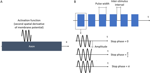
Figure 3. (A) Activating function in space applied to an axon for both continuous and pulse cases. (B) Activating function in time for pulsed study. Pulses of the same specified duration are separated by inter-stimulus intervals (pauses). A pulse has an important parameter which is a stop phase. The stop phase is a phase of an activating function that was applied at the last moment of pulse duration.
Download figure:
Standard image High-resolution imageIn the pulsed case, a short pulse of ultrasound was applied (figure 3(B)). The pulse duration was chosen to be  where
where  is a period of the ultrasound wave. The frequency was chosen to be
  as in the majority of the existing experimental studies.
We have investigated the influence of the stop phase and ultrasound pulse durations on the AP generation. Stop phase is a phase at which the ultrasound pulse is stopped, ranged from 0 to  as a phase of the sinusoidal function. In the finite element (FE) model it is a phase of an activating function which was applied at the last moment of each pulse for a pulsed ultrasound and at the last moment of a continuous ultrasound (which is equivalent to the physical meaning as far as the effect of ultrasound is approximated by the activating function).
A wide range of phases and amplitudes (table 1) were studied to understand the relationship between parameters and the generation and propagation of the AP, measured at  left from the ultrasound stimulated area for HH model and at
  for C-Fibre model.
Table 1. Parameter ranges for all studies.
| Study | Model | Parameters | |||||
|---|---|---|---|---|---|---|---|
Frequency, 
| Amplitude, 
| Pulse width, 

| Stop phase, 

| Inter-stimulus interval, 
| Number of pulses | ||
| Continuous | HH |

|

| ||||
| C-Fibre |

|

| |||||
| One pulse (amplitude and stop phase) | HH |

|

|

|

| ||
| C-Fibre |

|

|

|

| |||
| One pulse (pulse width) | HH |

|

|

|

| ||
| C-Fibre |

|

|

|

| |||
| Pulsed | HH |

|

|

|

|

|

|
| C-Fibre |

|

|

|

|

|

| |
| Pulsed (random phase) | HH |

|

|

|

|

|

|
| C-Fibre | |||||||
The influence of the pulse duration on the AP generation was investigated at frequencies of  and amplitudes of the activating function of
 for HH model and
 for C-Fibre model (the amplitudes were determined as a threshold for the AP generation for the respective models).
A series of pulsed ultrasound was applied for close resemblance to experiments and real applications (Gavrilov et al
1977, King et al
2013, Kim et al
2014, Blackmore et al
2019). Two new parameters were under investigation: number of pulses and duration of an inter-stimulus interval between pulses. Stop phase and duration of a pulse were also varied. Frequency and amplitude were chosen to be  and
and 
 for HH model and
  with different amplitudes for C-Fibre model.
Finally, the probabilistic behaviour of ultrasound stimulation was investigated. Stop phases were randomly distributed from 0 to  with the pulse length of
  periods, and inter-stimulus interval of
  Frequency and amplitude were 1
  and
and 
 respectively. The study was conducted only for the HH model as it was not possible to compute for the C-fibre due to computational difficulties.
3. Results
3.1. Examples and description of AP generation and propagation using continuous and pulsed ultrasound
Both HH and C-fibre models demonstrated that the proposed approach could reliably generate initiation and propagation of the AP. The ultrasound-induced APs were  and
and  in membrane potential for HH and C-fibre model respectively, and their corresponding velocities were
  and
and  which matches the literature for the typical slow-fibre APs (Hodgkin and Huxley 1952, Rosenthal and Bezanilla 2000, Tarotin et al
2019). The example studies demonstrated the stable AP initiation process and consequent propagation along the axon (figures 4–6) at various ultrasound modulation parameters.
which matches the literature for the typical slow-fibre APs (Hodgkin and Huxley 1952, Rosenthal and Bezanilla 2000, Tarotin et al
2019). The example studies demonstrated the stable AP initiation process and consequent propagation along the axon (figures 4–6) at various ultrasound modulation parameters.
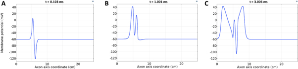
Figure 4. An example of the AP generation in the case of application a single-wave continuous ultrasound to the HH model. The ultrasound frequency was  the amplitude—
 (a) The initial phase at
  (b) The beginning of the AP generation at
  (c) The AP propagation in both directions from the point of generation at
  The resulting APs had membrane potentials equal
  and propagation velocities of
  which matched the classic Hodgkin–Huxley model.
Download figure:
Standard image High-resolution image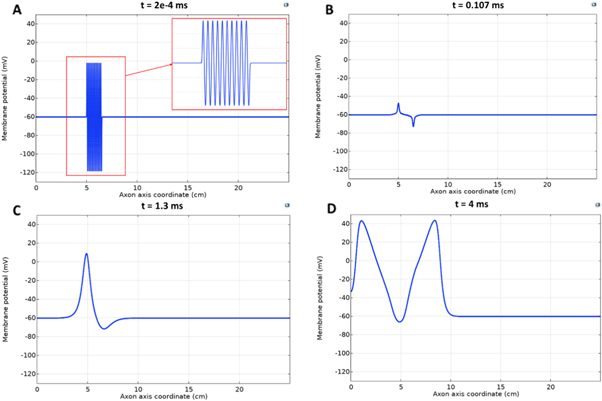
Figure 5. An example of the AP generation in the case of application of a pulsed ultrasound to the HH model. The ultrasound frequency was  the amplitude was

 pulses,
  periods each pulse,
  stop phase,
  inter-stimulus interval. (a) The initial phase at
  (b) The inter-stimulus interval between pulses at
  (c) The beginning of the AP generation at
  (d) The AP propagation in both directions from the point of generation at t = 4 ms. The resulting APs had membrane potential equals to
  and propagation velocities of
  which matches the classic HH model.
Download figure:
Standard image High-resolution image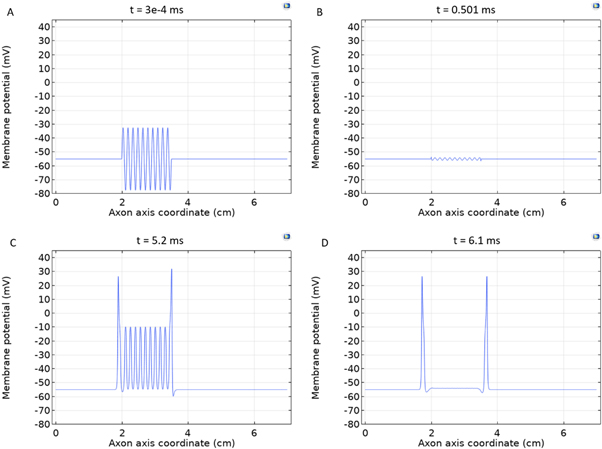
Figure 6. An example of the AP generation in the case of application of a pulsed ultrasound to the C-fibre model. The ultrasound frequency was  the amplitude was

 pulses,
  periods each pulse,
  stop phase,
 inter-stimulus interval. (a) The initial phase at
  . (b) The inter-stimulus interval between pulses at
  . (c) The beginning of the AP generation at
  . (d) The AP propagation in both directions from the point of generation at
  The resulting APs had membrane potential equals to
  and moving with the velocity of
  which matches the classic AP.
Download figure:
Standard image High-resolution imageThe comparison between standing and moving waves at frequencies of  with continuous ultrasound stimulation revealed that the standing wave has a lower threshold of AP generation by approximately half. At lower frequencies, this effect decreased so that below
  there was no significant difference between standing and moving waves. Significantly higher amplitude was required for AP generation at higher frequencies in the case of moving wave, doubling the one for the standing wave at frequencies above
  We were using a standing wave for the subsequent investigations as it was closer to the actual focused ultrasound used for neuromodulation.
3.2. Activation threshold in constant continuous ultrasound stimulation case
To find the activation threshold for the continuous ultrasound, different frequencies and amplitudes of activating function were applied for the whole duration of the simulation. The activating threshold varied with frequency (figure 7) and was  for
for  and increased to
  for
for  for the HH model, which corresponded to the mechanical strains of the axon by
  and
and  respectively. In figure 7 one can also find strain for each simulation case written in each cell. These strains show that an activation threshold in terms of strain is similar at all frequencies. However, there is a slight decrease of strains (from 0.68 to 0.41) for frequencies higher than
  The same analysis for the C-fibre resulted in the threshold
  for
for  and
and  for
for  respectively, which corresponded to
  and
and  mechanical strain. The activation threshold in terms of strain is similar at all frequencies for the C-fibre model.
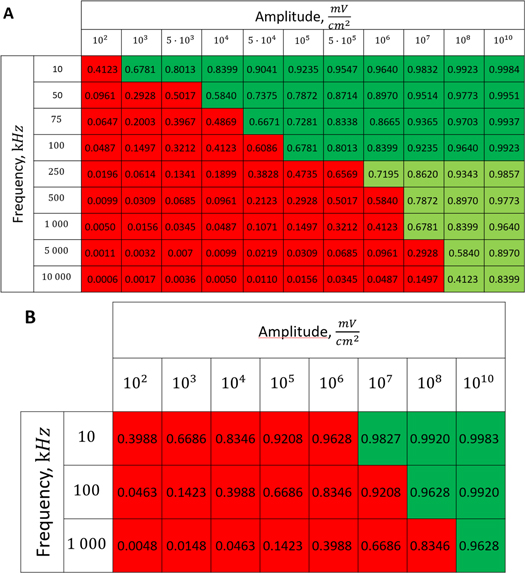
Figure 7. The summary of an axonal action potential generation test for a range of amplitudes and frequencies of a standing wave activating function boundary conditions (equation (13)). Red colour means no AP was generated, dark green—AP was generated, light green—AP should be generated but the model does not allow to simulate the generation and propagation due to the numerical constraints. Each cell contains strain in an axon for an exact frequency and amplitude. The strains are estimated with equation (14). (A) HH model. (B) C-fibre model.
Download figure:
Standard image High-resolution image3.3. Activation threshold in pulsed ultrasound stimulation case
3.3.1. Phase–amplitude relationship for the single pulse stimulation
The activation threshold for the pulsed ultrasound was found for different stop phases and the length of the pulse of  periods (
 ) at the frequency of 1 MHz (figure 8(A)). AP was generated when the amplitudes of the activating function were larger than
  (0.61 strain). The stop phases between
  and
and  (phases are expressed as a phase of sinusoidal function, see figure 3) caused the highest membrane voltage change and subsequent AP generation. This suggested that the generation of AP was more sensitive to the total energy translated to the system rather than the maximum membrane potential (figure 8, red dots). The highest energy value translated to the system was at the phase of
  (the wave stopped just after the positive phase), which corresponded to the highest membrane voltage for all amplitudes. The amplitudes of the activating function below
  (0.05 strain) did not significantly affect the membrane potential. For the C-fibre model the pattern was very similar (figure 8). Phases between
  and
and  were the most effective ones. The amplitudes below
  (0.8 strain) did not significantly change the membrane voltage.

Figure 8. The summary of an action potential generation for a range of stop phases and amplitudes of activating function. ultrasound was applied for the time of  periods and stopped at a specific stop phase (equation (14)) at a frequency of
  (A)–(C) Hodgkin–Huxley model. The maximal probe membrane potential recorded straight after stimulation at the probe location
  to the left of the stimulated zone. Red dots indicate the generation of an action potential after the stimulation. (D) C-Fibre model. Maximum membrane potential at a point
  mm to the left from the stimulated zone straight after ultrasound stimulation. Red cells indicate the generation of an action potential after the stimulation.
Download figure:
Standard image High-resolution image3.3.2. Pulse width analysis
Pulse widths and stop phases were varied at  with the activating function amplitudes
  (0.41 strain) and
  (0.8 strain) for the HH and C-Fibre models respectively (figure 9). The membrane potential in the HH model decreased with the increase of pulse width. As in the previous case, the stop-phase significantly affected the results with
  being optimal for the generation of the AP.
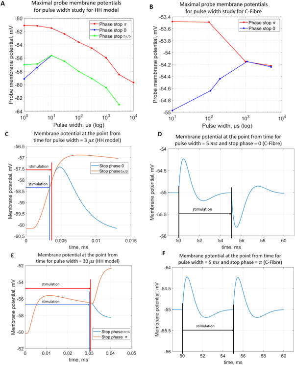
Figure 9. (A), (B) The summary of an action potential generation for a range of stop phases and durations of the activating function (A) of HH model at the amplitude of  (B) of C-Fibre model at the amplitude of
  (C)–(F) Membrane potentials at a point
  left from the stimulated zone with respect to time. (C) HH model, pulse width is
 stop phases are
  and
and  (D) C-fibre, pulse width is
  ms, stop phase is
  (E) HH model pulse width is
 stop phases are
  and
and  (F) C-fibre, pulse width is
  stop phase is
  The frequency was
  in all cases.
Download figure:
Standard image High-resolution imageC-Fibre model behaved differently (figure 9(B)). Membrane potential increased with the increase of a pulse width when the ultrasound was stopped at the zero stop phase. However, if the wave was stopped at  the membrane potential decreased with the increase of pulse width. When pulse width reached the length of
  periods there was no significant difference in the output between the two stop phases.
3.3.3. Analysis of the ultrasound modulation with pulse trains.
Here the activating thresholds and membrane potentials were investigated with respect to the number of pulses, pulse widths, stop phases, and interstimulus intervals (table 1) for the pulsed ultrasound delivered using the series of pulses, or a train (figures 10–12). A range of pulses of activating function with different widths was applied at  The amplitudes were
  (0.41 strain) for the HH model and
  (0.40–0.83 strain) for C-Fibre model.
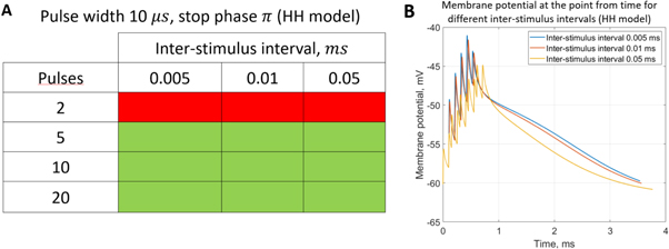
Figure 10. The summary of an axonal action potential generation for a range of number of pulses and inter-stimulus intervals of a standing wave pulsed activating function boundary conditions (equation (14)). (A) Red colour means no AP was generated, green—AP was generated.  periods (
 ) pulse width,
  stop phase, frequency—
 amplitude
  (B) Three different inter-stimulus intervals. Membrane potentials at a point
  left from the stimulated zone on time are presented. Frequency—
 amplitude
 pulses, pulse width =
  periods, stop phase =
  for each pulse.
Download figure:
Standard image High-resolution image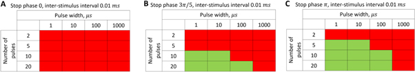
Figure 11. The summary of an axonal action potential generation of HH model for a range of number of pulses, stop phases and pulse widths of a standing wave pulsed activating function boundary conditions (equation (14)). Red colour means no AP was generated, green—AP was generated. Frequency  amplitude
  0.01 ms interstimulus interval. (A) stop phase
  (B) stop phase
  (C) stop phase
Download figure:
Standard image High-resolution image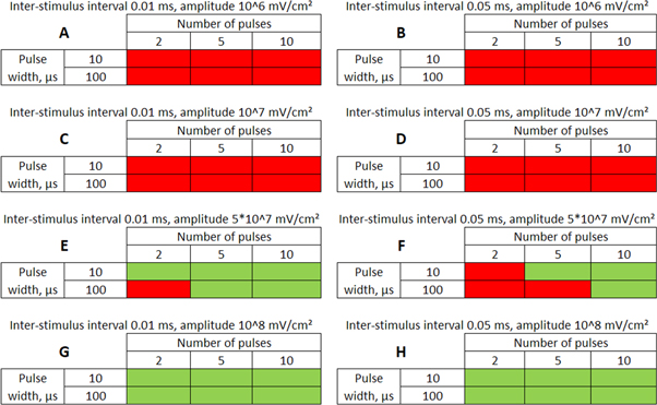
Figure 12. The summary of an axonal action potential generation of C-Fibre model for a range of number of pulses, pulse widths and stop pauses. Red colour means no AP was generated, green—AP was generated. Frequency  stop phase
  (A)
(A)  ms interstimulus interval and amplitude
  (B)
(B)  ms interstimulus interval and amplitude
  (C)
(C) 
 interstimulus interval and amplitude
  (D)
(D)  ms interstimulus interval and amplitude
  (E)
(E)  ms interstimulus interval and amplitude
  (F)
(F)  ms interstimulus interval and amplitude
  (G)
(G)  ms interstimulus interval and amplitude
  (H)
(H)  ms interstimulus interval and amplitude
Download figure:
Standard image High-resolution imageFor the HH model, inter-stimulus interval duration did not significantly affect the membrane voltage changes, however shorter inter-stimulus intervals resulted in generally higher membrane potentials (figure 10). The increase in the number of pulses was generally more effective in generating the AP (figure 11). Pulses for which the stop phase was  did not generate APs at all for our study parameters. The increase of a pulse width resulted in a significant decrease in the AP generation ability (figure 11).
C-Fibre model behaved in a similar way (figure 12). Amplitude had a major influence on the qualitative behaviour of the system. The number of pulses significantly changed the activating threshold at the amplitude of  (0.8 strain) (figures 12(E), (F)).
Additional experiment with  stop phase showed that axon did not generate the AP at amplitude 1
 pulses,
 interstimulus interval and
  periods (
 ) pulse width, whilst the AP was generated with a
  stop phase using the exact same parameters.
3.3.4. Phase–probability relationship: prediction of the experimental outcomes given random phase distribution per pulse.
In real experiments, the stop phase of the ultrasound sometimes is not controlled precisely and is therefore randomly distributed between the ultrasound pulses. This was modelled in the current subsection (figure 13) with the ultrasound pulses at a frequency of  with the amplitude of
  (0.43 strain), and with the
  ms interstimulus interval. The number of pulses and pulse width were varied respectively.
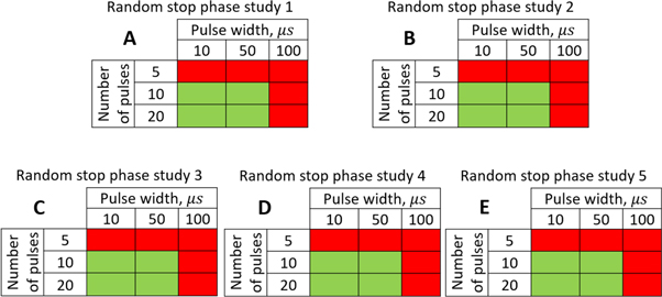
Figure 13. The summary of an axonal action potential generation for a range of the number of pulses and pulse widths of a standing wave pulsed activating function boundary conditions (equation (14)) with random stop phases. Red colour means no AP was generated, green—AP was generated. The frequency was 
 amplitude was
  interstimulus interval was
  Five cases with the same ultrasound stimulation parameters except for a random seed number generating random stop phases were simulated. (A)–(E) Studies 1–5.
Download figure:
Standard image High-resolution image
The stimulation of an axon had probabilistic nature, and the probability of AP generation significantly increased with a higher number of pulses ( and
and  ) and smaller pulse widths (mostly
  and
and  periods, figure 13).
4. Discussion
4.1. Summary of the results
The model of ionic concentration changes as a means of AP generation during ultrasound stimulation showed that this mechanism could indeed theoretically be responsible for ultrasound neuromodulation in a variety of cases. The continuous ultrasound case showed that the activating function amplitudes required for AP generation were  and
and  at
at  and
and  and
and  at
at  for HH and C-fibre models respectively. This corresponded to the strain values of
  and
and  at
at  and
and  and
and  at
at  The strains were equal at both frequencies, that indirectly supported the deformative nature of the effect of ultrasound stimulation on axons.
The pulsed ultrasound stimulation cases showed that the activation threshold varied with the stop phase, the number of pulses in the train, pulse width, and inter-stimulus interval. The stop phase had the most significant effect on the overall probability of AP generation, with the highest probability at the stop phase of  for both HH and C-fibre models.
The lowest thresholds for the AP generation with the pulsed ultrasound were  and
and  at
at  for HH and C-fibre models respectively, corresponded to the strain values of
  and
and  using the 5 pulses with 10 periods each, which were all stopped at
  stop phase. The analysis of the energy transfer in the system indicated that the first half of the sine wave generated the positive activating function which had a cumulative effect on the generation of the AP.
4.2. Answers to the stated questions
4.2.1. Can this mechanism be responsible for AP generation by ultrasound stimulation?
The feasibility and applicability of our results depend strongly on the assumption about the mechanical properties of the neural tissue, in particular the bulk compression modulus K. The literature proposes a range of contradicting results, with the values of K starting from  (obtained from the measured elastic modulus and Poisson's ratio under the assumption that the brain tissue is an isotropic linear elastic body) (Miller and Chinzei 2002), and up to the highest value
  obtained from the measurement of the speed of ultrasound wave propagation (Etoh et al
1994).
obtained from the measurement of the speed of ultrasound wave propagation (Etoh et al
1994).
This in turn leads to a range of possible amplitudes of mechanical strains. On one hand, if  takes a relatively small value, acoustic pressures typically produced by ultrasound stimulating machines could lead to extremely large deformations (strains close to
  ). On the other hand, probably the more realistic values of mechanical properties are close to those of water. That is also supported by ultrasound propagation speed (Etoh et al
1994, Zoric et al
1999, Ganpule et al
2018, Reyes Hernandez et al
2018), and in this case, typical ultrasound pressures cannot induce strains above 0.01 (
). On the other hand, probably the more realistic values of mechanical properties are close to those of water. That is also supported by ultrasound propagation speed (Etoh et al
1994, Zoric et al
1999, Ganpule et al
2018, Reyes Hernandez et al
2018), and in this case, typical ultrasound pressures cannot induce strains above 0.01 ( ). According to this assumption, the concentration hypothesis does not produce any significant effects because deformations in the tissue cannot reach high enough values to achieve a certain level of activating function amplitude. However, in such a situation, the effect of cavitation can occur which would drive the deformations high enough to be the prime cause for AP generation, even before the intermembrane cavitation happens.
Other studies have shown that high enough strains are possible in the brain tissue (Miller et al 2000, Miller and Chinzei 2002, Soza et al 2004, Laksari et al 2012, Morin et al 2017), and thus the ionic concentration effect could as well be responsible for the observed experimental effects. Concerning the peripheral nerve axons specifically, the existing literature suggests that strains can reach 1 (100%) under the application of the ultrasound (Julian and Goldman 1962, Downs et al 2018), which would match our predictions. However, this requires further verification and additional carefully conducted and controlled experiments.
Moreover, the acoustic radiation force, which can be computed as a dependant parameter in our study was shown to be the prime factor causing neurostimulation according to Menz et al (2019). This radiation force may cause deformations in an axon and its surroundings which may lead to concentration changes. This is supported by the fact that in Menz et al (2019) neurostimulation effect increases with an increase in the ultrasound frequency, which was also observed in the present study.
Further experiments are required to confirm or reject the possibility of the concentration mechanism to be responsible for AP generation by ultrasound stimulation.
4.2.2. What are the implications for the experimental predictions?
Although this study could not provide an exact answer to this question due to the absence of the direct experimental evidence, our results could explain and simulate a range of observed experimental effects (see below) without involving any alternative mechanisms, and with specific tuning could also seamlessly incorporate effects of the cavitation. The qualitative behaviour of the AP generation predicted by the approach matched closely the range of experimentally observed effects. Specifically, the increase of neurostimulation effect with the increase of the frequency (Menz et al 2019), strong dependence of the effect of ultrasound on its intensity, the increase of neurostimulation effect with the decrease of the pulse duration (Wright et al 2015, 2017, Downs et al 2018) and the possibility to initiate the AP with low duration pulses (Tyler et al 2008, Vion-Bailly et al 2019). In addition, the probabilistic nature of ultrasound stimulation of unmyelinated peripherical nerves shown in Wright et al (2017) was directly predicted by our model when random stop phase was employed, which simulated the realistic ultrasound parameters. The small qualitative difference there could be explained by different axon parameters.
Our approach is based on a conventional electrical stimulation model, which fits well with the experimental evidence showing that ultrasound and electrical stimulation methods have common effects on axons (Downs et al 2018). Finally, experiments show (Galbraith et al 1993) that membrane potential depends on strain and strain rate which corresponds well to the proposed mechanism and also validates the dependence of AP generation on a frequency of ultrasound.
The results and the models can be used directly to create a realistic FE model of ultrasound stimulation of a subdiaphragmatic vagus nerve and nociceptors. It is planned to directly verify our results in subdiaphragmatic vagus nerve through ex vivo and in vivo experiments.
Specific attention should be brought to the obtained activating-phase relationship, which favours phases close to  This, together with the probabilistic nature of pulsed ultrasound phase control, could explain the apparent probabilistic nature of the AP generation in the experiments mentioned by King et al (2013), Blackmore et al (2019), Vion-Bailly et al (2019).
We are planning to design an experiment, where the phase of the ultrasound will be controlled precisely. This could decisively test the question about the prime mechanisms responsible for neurostimulation because if this is intermembrane cavitation, the results would stay probabilistic even in the controlled case conditions, contrary to the proposed approach where results would strongly depend on the phase.
We are also planning to design the experiment for the exact measurement of the strain occurring in neural tissue during the propagation of the ultrasound which could point to the feasibility and applicability of the proposed approach.
4.3. Technical limitations
Here we only considered unmyelinated fibres. We also greatly simplified the transition between mechanical strain and boundary conditions. Although we are confident about the qualitative results, we need to develop a more complicated model in order to study the quantitative effects thoroughly. The one-to-one comparison to other hypotheses would be ideal, however, this is challenging given the fact that most parameters for the other hypotheses are usually obtained experimentally.
4.4. Future work
In future, we are planning to extend the model for the simultaneous solution of Nernst–Plank equations and HH (and C-fibre) equations. We are also planning to create a myelinated coupled electro-acoustic model of the axon. We then are planning to confirm the qualitative results obtained in this work, obtain predictive quantitative results for particular nerves, and conduct an experimental study which would definitively answer the question on the exact influence of the ionic concentration mechanism on neurostimulation by the ultrasound.
One of the potential applications of ultrasound stimulation could be the possibility of affecting the direction of the information flow within the vagus nerve. For example, the threshold of stimulation could be different for A-delta efferent fibres and the rest of the myelinated fibres. Existing models of myelinated fibres (McIntyre et al 2002) offer the possibility of such investigations. We therefore will consider the possibility of assessing this and comparing the myelinated and unmyelinated fibre behaviour.
Acknowledgments
This research work was supported by the Academic Excellence Project 5-100 proposed by Peter the Great St. Petersburg Polytechnic University.