
Abstract
Objective. Low-dose computed tomography (LDCT) denoising is an important problem in CT research. Compared to the normal dose CT, LDCT images are subjected to severe noise and artifacts. Recently in many studies, vision transformers have shown superior feature representation ability over the convolutional neural networks (CNNs). However, unlike CNNs, the potential of vision transformers in LDCT denoising was little explored so far. Our paper aims to further explore the power of transformer for the LDCT denoising problem. Approach. In this paper, we propose a Convolution-free Token2Token Dilated Vision Transformer (CTformer) for LDCT denoising. The CTformer uses a more powerful token rearrangement to encompass local contextual information and thus avoids convolution. It also dilates and shifts feature maps to capture longer-range interaction. We interpret the CTformer by statically inspecting patterns of its internal attention maps and dynamically tracing the hierarchical attention flow with an explanatory graph. Furthermore, overlapped inference mechanism is employed to effectively eliminate the boundary artifacts that are common for encoder-decoder-based denoising models. Main results. Experimental results on Mayo dataset suggest that the CTformer outperforms the state-of-the-art denoising methods with a low computational overhead. Significance. The proposed model delivers excellent denoising performance on LDCT. Moreover, low computational cost and interpretability make the CTformer promising for clinical applications.
Export citation and abstract BibTeX RIS

Original content from this work may be used under the terms of the Creative Commons Attribution 4.0 licence. Any further distribution of this work must maintain attribution to the author(s) and the title of the work, journal citation and DOI.
1. Introduction
The Low-dose computed tomography (LDCT) problem has gained lots of attention in the community due to its potential of reducing x-ray radiation. However, compared to normal dose CT (NDCT) images, LDCT images suffer from severe noise and artifacts (Brenner and Hall 2007) when they are applied to clinical applications. To overcome this problem, two types of algorithms have been investigated: traditional algorithms and convolutional neural networks (CNNs) (He et al 2016a, Fan et al 2021a). (i) Traditional algorithms such as iterative methods suppress the artifacts and noise by using a physical model based on a certain prior. Unfortunately, these algorithms are hard to be adopted in commercial CT scanners because of the hardware limitations and high computational cost (Yin et al 2019). (ii) With the advent of deep learning, CNNs have been a prevailing approach for LDCT image denoising. Despite the superior learning ability aided by big data (Wang et al 2020), CNNs are reported to be limited in capturing long-range contextual information in images (Vaswani et al 2017, Wang et al 2018, Liu et al 2021, Yuan et al 2021), which will adversely affect the retrieval of richer structural information in denoised images.
Recently, the transformer model (Vaswani et al 2017) has shown excellent performance in computer vision (Chen et al 2020a, et al , 2020b, Chen et al 2020b, Dosovitskiy et al 2020, Touvron et al 2020, Yang et al 2020, Chu et al 2021, Wu et al 2021, Cao et al 2021, Han et al 2021). Dosovitskiy et al proposed the first vision transformer (ViT) by simply mapping an image into 16 × 16 patches (this operation is commonly referred to as tokenization) in analogy to words in a sentence in natural language processing (Dosovitskiy et al 2020). Yuan et al further proposed a Token2Token method to empower the transformer model with a diverse information encoding (Yuan et al 2021). Next, Liu et al designed a swin transformer to include patch fusion and cyclic shift to enlarge the perception of contextual information in tokens (Liu et al 2021). Moreover, Choromanski et al proposed a Performer transformer to reduce the computational complexity of the self-attention by approximating the inherent softmax operator (Choromanski et al 2020b). Currently, the transformer model is poised to replace CNNs as the mainstream deep learning model. On the one hand, compared to CNNs, the transformer model is good at capturing global information and long-range feature interactions, resulting in the utilization of richer information. As shown in figure 1, the transformer has diversified and effective features, while the CNN model has many inactive features. On the other hand, the transformer model enjoys higher visual interpretability by the virtue of its inherent self-attention block (Montavon et al 2019, Abnar and Zuidema 2020, Chefer et al 2021). However, a typical CNN model contains no generic explanation modules (Fan et al 2021b).

Figure 1. The feature maps visualization of the pretrained RED-CNN and the CTformer. The transformer model (CTformer) has diversified and effective features, while the CNN model (RED-CNN) has a lot of inactive features.
Download figure:
Standard image High-resolution imageIn our opinion, the transformer model is suitable for LDCT denoising problem. Other than the effectiveness, a transformer is more desirable for physicians because it is self-explanatory (Singh et al 2020), e.g. allowing a physician to make sense of the model's inner logic. Currently, there are several pieces of research that explored the transformer models in LDCT denoising (Zhang et al 2021b, Luthra et al 2021, Li et al 2022a, Wang et al 2022, Yang et al 2022). Zhang et al pioneered to apply the transformer modules on the outcomes of the Gaussian filter and facilitate LDCT denoising (Zhang et al 2021b). Luthra et al adopted the Sobel-Feldman operators and the LeWin transformer to optimize the noise residual information in LDCT (Luthra et al 2021). Yang et al proposed a sinogram inner-structure transformer to attenuate the LDCT noise by exploiting the inner-structure in the sinogram domain (Yang et al 2022). Next, Li et al devised a dual branch model with the overlapping-free window-based self-attention transformer block on the main branch and an enhancement module to improve the edge, texture, and context information in the LDCT images (Li et al 2022a).
However, all these work neglected the transformer's interpretability which is crucial for clinical applications (Kim et al 2019). In this paper, we aim to explore both the efficacy and interpretability of transformers in LDCT denoising. Specifically, we propose a Convolution-free Token2Token Dilated Vision Transformer (CTformer) for low-dose CT denoising. The following traits apply to the CTformer: (i) since the pure transformer model is easier to understand than a hybrid one, the convolutional modules are omitted in the proposed CTformer to better investigate the model interpretability. Although convolution is instrumental to capture local features when it is combined with transformers, it is not a necessity because the token rearrangement component in CTformer can also support local information fusion. To the best of our knowledge, the CTformer is the first pure transformer for LDCT denoising. (ii) The dilation and a cyclic shift are used in the Token2Token to enlarge the receptive field, thereby gaining broader contextual information from the feature maps and reducing the computational cost. (iii) We utilize an overlapped inference mechanism to address the boundary artifact that is common in the encoder-decoder denoising models. (iv) We develop interpretability for the CTformer with the visual attention maps and an explanatory graph that shed light on how the CTformer discriminates key structures from noise as well as hierarchical attention flow across layers. Experiment results suggest that the CTformer delivers superior denoising performance over other state-of-the-arts with fewer trainable parameters and multiply-accumulate operations (MACs).
In summary, our contributions are threefold: (i) this work is the forerunner to apply the vision transformer to LDCT denoising problem. What's more, the proposed CTformer is the first pure transformer. (ii) We introduce dilation and cyclic shift to enhance the tokenization process in the model, utilize a new inference mechanism to fix the boundary artifacts, and develop the interpretation methods to unveil the model's denoising patterns. (iii) Our experimental results demonstrate the superior denoising performance and model efficiency of the CTformer for LDCT denoising.
Please note that this manuscript is an extension of our previously-published conference paper Ted-net: Convolution-free t2t vision transformer-based encoder-decoder dilation network for low-dose ct denoising (Wang et al 2021b), which is a pioneer exploration of transformer models in LDCT denoising. Compared to the previous conference version, this paper added more extensive analysis and experiments for the proposed model. Specifically, we added three more sections including the overlapped testing, model efficiency, and model Interpretability. These parts further demonstrated the high efficacy and efficiency of the proposed model.
2. Related work
The previous studies for the LDCT denoising problem can be categorized into two classes.
Traditional algorithms. Typically, these methods incorporate a physical prior into an iterative reconstruction framework to suppress noise. For example, compressed sensing (CS) has been widely used for the LDCT problem by adopting a sparse representation (Yu and Wang 2009), i.e. the total variation minimization assumes that the clean image is piecewise constant whose gradients are sparse (Sidky and Pan 2008, Tian et al 2011, Liu et al 2012, Zhang et al 2014). Xu et al used a dictionary to construct the sparse representation (Xu et al 2012) for LDCT denoising. In addition to the sparsity prior, Ma et al designed a non-local mean prior to utilize the image voxels across the whole image rather than the local region (Ma et al 2011). However, increasingly more studies (Chen et al 2017, Wu et al 2017, Yang et al 2018, Fan et al 2019) implied that the traditional algorithms are surpassed by deep learning models driven by big data.
Convolution models. CNNs have been used for the LDCT image reconstruction. Wu et al used a K-sparse autoencoder to learn the image features in an unsupervised fashion and minimize the distance between a normal-dose image and an iterative reconstruction result in the feature space of the autoencoder (Wu et al 2017). Liu et al proposed a 3D residual convolutional network to estimate an iterative reconstruction (IR) image from an LDCT analytic reconstruction image (Liu et al 2019). Their method can save time because it avoids the time-consuming iterative reconstruction. He et al proposed the 3pADMM method to address the problems of hyper-parameter optimization and prior knowledge selection in LDCT reconstruction (He et al 2018).
Besides, a majority of deep LDCT denoising models focused on image post-processing. The paper of Chen et al was a pioneer work which employed the convolution, deconvolution, and shortcut connections to prototype a residual encoder-decoder convolution neural network (RED-CNN) (Chen et al 2017). Yang et al used the generative adversarial network with Wasserstein distance (WGAN) aided by a perceptual loss to improve the quality of denoised images (Yang et al 2018). Due to the excellent performance of WGAN in generating faithful real-world CT images and the role of the perceptual loss in structural fidelity, this model alleviated the over-smoothness in the denoised images. Li et al employed a GAN armed with the structural similarity loss, the perceptual loss, the adversarial loss, and the sharpness loss to preserve structural details and sharp boundaries (Li et al 2021). Fan et al constructed a quadratic neuron-based autoencoder for LDCT image denoising with more robustness and efficiency as opposed to conventional CNN-based methods (Fan et al 2019). It is the first autoencoder based on a new type of neurons. Huang et al proposed a two-stage residual CNN (Huang et al 2020), where the first stage uses stationary wavelet transform for texture denoising, and the second one enhances the image structure via combining the average of NDCT images and the denoised image from the first stage.
However, CNN-based models typically lack the ability to capture global contextual information due to the limited receptive fields, thus less efficient to model the structural similarity across the whole image (Wang et al 2021a, 2021b, Zhang et al 2021b).
3. Methods
In the supervised setting, with a deep learning model, the LDCT denoising task is to learn a mapping from a paired noisy LDCT image x to a clean NDCT image y . Mathematically, a neural network can be trained by optimizing a mean square error (MSE) loss function as follows:

where f( W ; x ) is a neural network, and W is a collection of parameters for simplicity.
3.1. Architecture of the CTformer
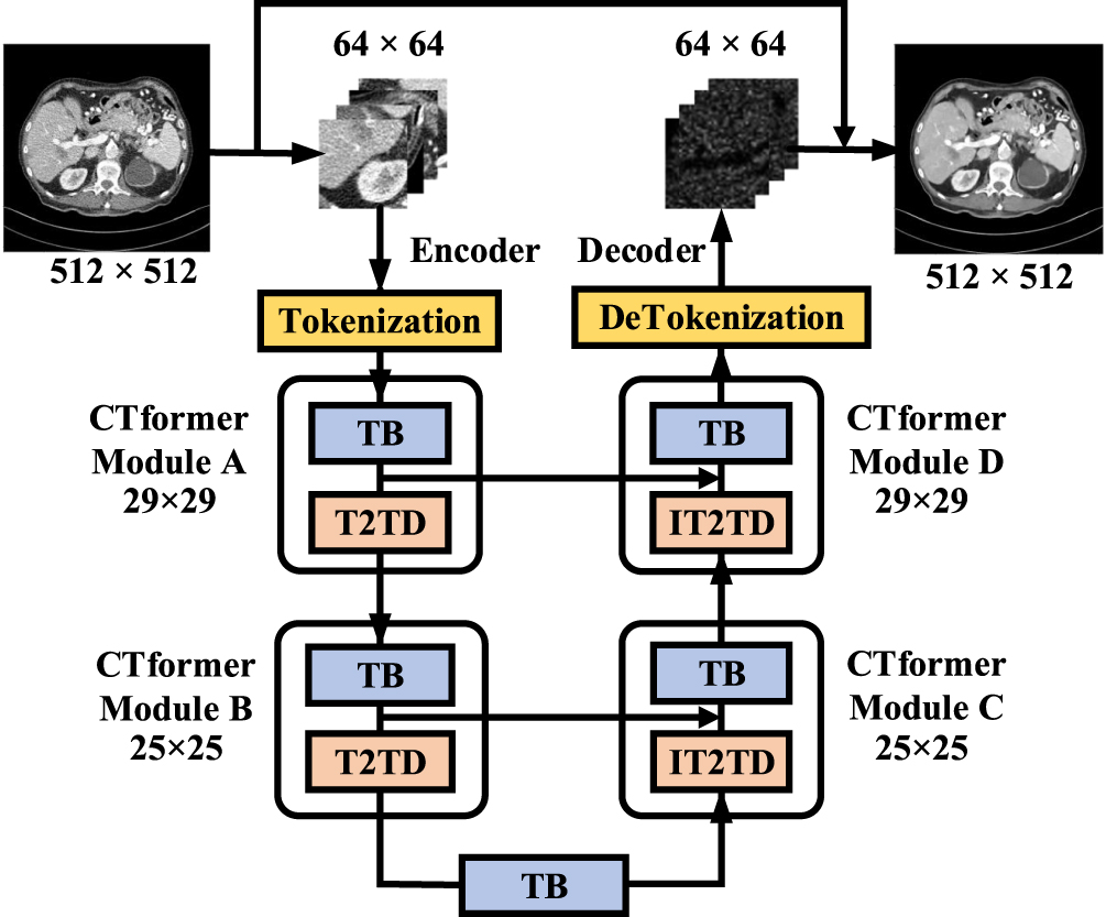
As shown in figure 2, the proposed CTformer takes the residual encoder-decoder structure with tokenization/detokenization blocks, four CTformer modules, and an intermediate transformer block. In the encoder, CTformer modules A and B include a transformer block (TB), and a Token2Token Dilation block (T2TD). In the decoder, CTformer modules C and D symmetrically encompass an inverse Token2Token Dilation block (IT2TD) and a TB. The IT2TB block takes the inverse design of the corresponding T2TB block. Now let us introduce the CTformer from its macro to micro structures.

Figure 2. The CTformer consists of the residual encoder-decoder structure with tokenization/detokenization blocks, four CTformer modules with different sizes of feature maps, and an intermediate transformer block. Tokenization block unfolds image patches into sequential tokens, while detokenization block converts tokens back to the image. Each encoder CTformer module includes a transformer block (TB) and a Token2Token dilation block (T2TD), while each decoder CTformer module consists of an inverse Token2Token dilation block (IT2TD) and a TB, symmetrically.
Download figure:
Standard image High-resolution imageResidual encoder-decoder structure. We use a residual encoder-decoder structure as the backbone of the CTformer. The shortcuts only bridge similar levels of layers in encoder and decoder parts. Although the unsatisfactory information loss is accompanied by denoising in the encoder block, which hurts the structural recovery in the decoder part, the employment of shortcuts can supplement information from the feature maps of the encoder to retain structural details. Besides, shortcuts can fix the gradient vanishing problem such that a deep model can still be stably trained (He et al 2016b).
Tokenization block. As shown in figure 3, in the tokenization process, a noisy CT image is unfolded into a sequence of two dimensional (2D) patches (also referred to as tokens):  , where b is the batch size, n is the number of tokens, and d0 is the token dimension. Throughout this manuscript, we use tokens and patches interchangeably.
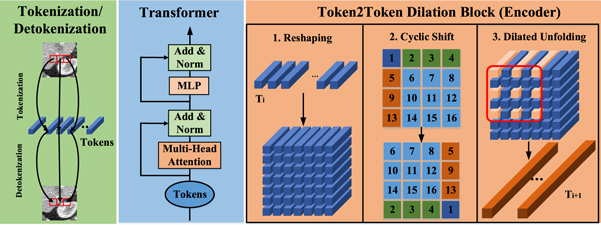
Figure 3. The micro structures of the CTformer: tokenization/detokenization, transformer block and Token2Token dialtion block.
Download figure:
Standard image High-resolution image
Transformer block. As shown in figure 3, a typical transformer block contains multiple head attention (MHA), layer normalization (LN), an MLP, and residual connections to enhance the expressive power. Specifically, in the self-attention, a token sequence  is linearly mapped into three tensors which are respectively referred to as query, key, and value, denoted as
  for short, where dm
is the token embedding dimension. Mathematically, we have
for short, where dm
is the token embedding dimension. Mathematically, we have

where Wq , Wk and Wv are linear operators. Then, the output of the self-attention is calculated as

where the scaling factor  is based on the network depth. Besides the authentic calculation of equation (3), the
  operator can be approximated by a kernel method, thus, obtaining a reduced complexity of equation (3). The transformer using this approximation is also called Performer (Choromanski et al
2020b).
operator can be approximated by a kernel method, thus, obtaining a reduced complexity of equation (3). The transformer using this approximation is also called Performer (Choromanski et al
2020b).
 is the attention map that will be used in the post-hoc interpretability analysis. Through the transformer block, the output token
  is
is

Token2Token dilation block. Previously, the simple tokenization in the vanilla transformer only includes one tokenization process using either reshaping or convolutions with a fixed stride to convert an image to tokens. Thus, it tends to ignore the dependence across neighboring tokens. What's worse, it also makes the attention expressions redundant, which adversely results in limited feature richness in each layer (Yuan et al 2021). To overcome these problems, as shown in figure 3, we adopt the recently-proposed T2T block which uses cascade tokenization to replace the simple tokenization (Yuan et al 2021). The T2T block consists of reshaping and unfolding which cannot only model the local information from the surrounding image pixels but also gain more feature representation than convolution. Furthermore, we use cyclic shift and dilation in the T2T dilation block (T2TD) to refine the contextual information fusion and leverage spatial relations across a larger region. Now, let us elaborate on these operations in detail.
Step 1: reshaping . A sequence of tokens  given rise by the transformer block are first transposed to
  and then reshaped into
  :
:

where  are the height and width of the feature map, respectively.
Step 2: cyclic shift . Due to its capacity to take advantage of the potential circulant similarity in noise patterns, the cyclic shift or cycle spinning has been proven to be effective at removing noise from signals (Fletcher et al 2002, Chen et al 2015). In this paper, we also employ the cyclic shift to facilitate information fusion in the proposed model. Specifically, the pixel values in the feature maps are shifted in a cyclic way to utilize the information more sufficiently. Through cyclic shift, the tokens fed into the consequent transformer blocks are extracted from various feature maps rather than the fixed patches. For example, now the tokens from the boundaries of the modified feature maps include pixels that are not boundaries in the original feature maps. Figure 3 illustrates the cyclic shift module

Step 3: dilated unfolding . The dilated unfolding will use the unfolding operation to retokenize the feature maps from the last step. To alleviate the information loss in this step, we adopt an overlapped splitting of patches. As a result, these aggregated tokens can respect the correlations among the neighboring tokens

In this stage, the 4D feature maps  are converted back to 3D tokens
  , where ns
and ds
represent the new token number and token dimension, respectively. By aggregating surrounding patches and pixels, the local information is favorably preserved, and the number of tokens is changed. Specifically, the token number decreases in the encoder and increases in the decoder.
, where ns
and ds
represent the new token number and token dimension, respectively. By aggregating surrounding patches and pixels, the local information is favorably preserved, and the number of tokens is changed. Specifically, the token number decreases in the encoder and increases in the decoder.
Instead of the regular unfolding, we endow the unfolding with a dilation to capture the longer range contextual information with less computational cost. Mathematically, the perceptive field P of the dilation can be calculated as follows:

where Ki
and Di
denote the kernel size and the dilation rate in a certain dimension, respectively. After the dilated unfolding, the input feature map  becomes
  , where dsd
= d × ∏i
Ki
and the total number of tokens nsd
after the dilated unfolding operation is calculated as:
, where dsd
= d × ∏i
Ki
and the total number of tokens nsd
after the dilated unfolding operation is calculated as:

where  is the floor function, spatial(i) means corresponding size in the i dimension, spatial(0) = h in height dimension, and spatial(1) = w in width dimension. Here, dilation, kernel, and stride are related parameters in the unfolding operation. Then, an MLP is performed to map the embedding dimension to the desired size.
3.2. Inference of the CTformer
In the inference phase, unlike CNN which can directly test the whole image, the transformer model can only do inference patch by patch. Because there exists information loss in the bottleneck of an encoder-decoder architecture (Innamorati et al 2020), the denoised results of these patches are inconsistent at boundaries, causing boundary artifacts in the stitched image. As shown in figure 4, we can easily see the mosaic edge indicated by the red arrows, and artifacts are along all four directions. To address this problem, we employ the overlapped inference method. The core of our method is to discard the margin and only keep the center of the model output to stitch the final prediction.

Figure 4. (a) The residual map between the prediction and the NDCT image reveals the boundary artifacts. (b) The profiles of the residual map along the horizontal and vertical axes.
Download figure:
Standard image High-resolution imageSuppose that the patch size is p × p, we only keep the central part of a patch (p − 2η) × (p − 2η) to form the final prediction image, where η is selected to be greater than the width of artifacts. In the overlapped inference, slightly more calculations are demanded because we discard the peripheral part of a patch. The increased cost is at the ratio of

where n is the original image size, and ⌈ · ⌉ is the ceiling function. Therefore, we need to balance the computation cost with the artifact elimination effect.
3.3. Interpretability of the CTformer
In interpretability research, saliency map is the most popular method. One can generate a saliency map for the CNN-based classification model after the model is trained (Selvaraju et al 2017). However, for the image-to-image denoising task, deriving saliency maps are not applicable because denoising models are essentially regression models. In contrast, even if the transformer models are used for denoising, one can leverage the inherent attention modules to achieve saliency maps. Utilizing such an advantage, we develop the interpretability of the CTformer by probing the patterns of the attention maps. Thus, one can decode the inner-working of the CTformer, with an emphasis on the processing of important structural and semantic information. The self-interpretability makes the CTformer uniquely relative to other LDCT denoising models.
Furthermore, we observe that the attention only reflects where the model attends in a static manner, which cannot convey how the attended parts flow across layers in the CTformer. To complement this dynamic information, inspired by Zhang et al (2021a), we propose to construct an explanatory graph to describe the hierarchical flow of the attention. We take the attended parts as graph nodes and the attention flow as graph edges. Two nodes linked by an edge are usually co-activated and take similar mapping (denoising). Specifically, we first recognize the attended object parts by identifying the peak activations. Then, we build the graph connections between neighboring layers by forwarding a masked feature map and monitoring the high activations.
Node: to identify the object part, we provide two pixel-based methods: TopK and local maximum (LM) selection. The TopK extracts the K-highest activation across the attention maps, while the LM detects the local maximum activations.
Edge: to construct edges among nodes, we propose to forward a masked feature map. Specifically, given a node (an object part) in a layer, we mask the feature maps and only keep the region around the node. Then, we feed the masked feature maps to obtain the attention map of the next layer. Finally, we extract the highest activation (node) from the obtained attention map and link it to the given node.
By performing the above steps recursively in two subsequent layers, the whole explanatory graph is built to inform us how the attention of the CTformer is shifted.
4. Experiments
In this part, our model is trained and evaluated on a publicly available dataset. First, we demonstrate the superior denoising performance and the model efficiency of the CTformer over its counterparts. Then, we confirm the effectiveness of the overlapped inference mechanism. Finally, we elaborate on the model interpretability with the aforementioned interpretation methods.
Dataset. A publicly released dataset from 2016 NIH-AAPM-Mayo Clinic LDCT Grand Challenge 5 (McCollough et al 2017) is used for model training and testing. The dataset includes 2, 378, 3.0 mm slice thickness of low-dose (quarter) and normal-dose (full) CT images from ten anonymous patients. Cross-validation is applied for model evaluation where nine patients are used for model training, and one patient for testing. Additionally, random rotation and flipping are performed on the primary images as part of data augmentation.
Experiment settings. We list the detailed experimental settings in the following:
- The experiments are running on Ubuntu 18.04.5 LTS, with Intel(R) Core (TM) i9-9920X CPU @ 3.50 GHz using PyTorch 1.5.0 (Paszke et al 2019) and CUDA 10.2.0. The model is trained with four NVIDIA GTX 2080Ti 11G GPUs.
- The intermediate transformer block takes the authentic design, while the transformer blocks in the CTformer modules take Performer to facilitate model training. The embedding dimension for all transformer blocks is 64.
- In tokenization/detokenization, the kernel for the unfolding/folding is set to 7 with a stride of 2 to reduce computational cost. For the four CTformer modules, the cyclic shift strides in the T2TD/IT2TD blocks are {2, 2, −2, −2}. The kernel sizes of the unfolding/folding operations are 3 with dilations of {2, 1, 1, 2}, respectively. The strides are set to 1 to avoid the information loss. Thus, according to equation (9), the corresponding token numbers n1, n2, and n3 for the CTformer module A, CTformer module B, and the intermediate transformer layer are computed as follows:here
 and can be calculated from the reshaping process in equation (5). The transformer token numbers in the decoder are symmetrically arranged as {625, 841}.
 - We randomly extract 4 patches from all available slices for training through 4000 epochs with a batch size of 16. In a training batch, fewer patches with more images lead to less fluctuations and bias than more patches with fewer images because many patches from a single image usually cannot represent the overall data distribution.
- Adam is adopted to minimize the MSE loss with an initial learning rate of 1.0 × 10⁻⁵, which gradually decreases to 1.0 × 10⁻⁶ with a scheduled decay rate.
- A margin size of 16 is used for overlapped inference.


Denoising performance. The performance of the CTformer is compared to other state-of-the-arts, e.g. RED-CNN (Chen et al 2017), WGAN-VGG (Yang et al 2018), MAP-NN (Shan et al 2019), and AD-NET (Tian et al 2020). The selected models are all popular low-dose CT or natural image-denoising models that were published in flagship journals. We retrain all the models based on their officially-disclosed codes. Please be informed that we are unable to compare the CTformer to other transformer-based LDCT denoising models due to the closed source barrier and distinct model framework.
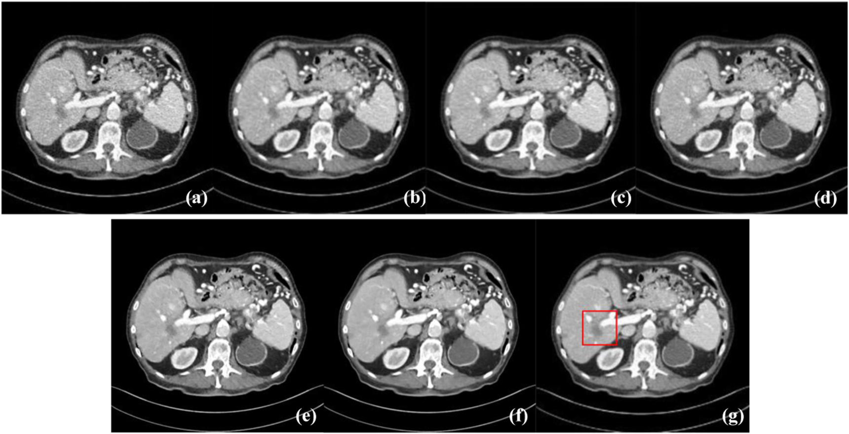
Figure 5 shows the results of different networks on L506 with Lesion No. 575, and figure 6 demonstrates the ROIs from the rectangular area marked in figure 5. It can be seen that all methods can alleviate noise and artifacts to some extent, but the CTformer generates the clearest and the most perceptually-pleasing denoised images. Specifically, per the ROIs from figure 6, we find that WGAN-VGG and MAP-NN seem to introduce additional shadows and tissues. While RED-CNN and AD-NET produce a smoother and clearer image relative to WGAN-VGG and MAP-NN, there still exists blotchy noise around the lesion. In contrast, the CTformer satisfactorily suppresses the noise and artifacts, maintains high-level spatial smoothness, and keeps the structural details in the restored image. Therefore, we conclude that the CTformer is one of the best denoisers compared to its competitors.

Figure 5. The denoised results of different networks on L506 with Lesion No. 575. (a) LDCT, (b) RED-CNN, (c) WGAN-VGG, (d) MAP-NN, (e) AD-NET, (f) the proposed CTformer, and (g) NDCT. The display window is [−160, 240] HU.
Download figure:
Standard image High-resolution image
Figure 6. The ROIs of the rectangle marked in figure 5. (a) LDCT, (b) RED-CNN, (c) WGAN-VGG, (d) MAP-NN, (e) AD-NET, (f) the proposed CTformer, and (g) NDCT.
Download figure:
Standard image High-resolution imageAdditionally, two metrics: structural similarity (SSIM) and root mean square error (RMSE) are adopted to quantitatively assess the quality of the denoised images. For fairness, we evaluate the model complexity with the number of trainable parameters (#param.) and MACs. Table 1 shows the average SSIM and RMSE on all slices of L506. Among the state-of-the-art methods, only AD-NET achieves an SSIM score over 0.91, and only MAP-NN and AD-NET have an RMSE score below 10. In contrast, our CTformer has the highest SSIM of 0.9121 and smallest RMSE of 9.0233. Concerning model complexity, MAP-NN has the highest MACs of 13.79 G because it uses a lot of repeated modules, while WGAN-VGG has the greatest number of trainable parameters of 34.07 M because it uses VGG as a feature extractor. In contrast, the CTformer has the smallest number of parameters and the lowest MACs. Compared to its competitors, our model has the best performance with the lowest computational cost.
Table 1. Quantitative evaluation results of different methods on L506 using SSIM and RMSE. The bold-faced numbers are the best results.
| Method | #param. | MACs | Throughput | SSIM ↑ | RMSE ↓ |
|---|---|---|---|---|---|
| LDCT | — | — | — | 0.8759 | 14.2416 |
| RED-CNN | 1.85 M | 5.05 G | 1.74 Im s−1 | 0.9077 | 10.1044 |
| WGAN-VGG | 34.07 M | 3.61 G | 2.26 Im s−1 | 0.9008 | 11.6370 |
| MAP-NN | 3.49 M | 13.79 G | 1.96 Im s−1 | 0.9084 | 9.2959 |
| AD-NET | 2.07 M | 9.49 G | 1.23 Im s−1 | 0.9105 | 9.0997 |
| CTformer | 1.45 M | 0.86 G | 1.43 Im s−1 | 0.9120 | 9.0223 |
Inference speed. Furthermore, model throughput is used as a metric to show the quantity of images the model can process in a unit time (Im s−1). The results in table 1 show that the inference efficiency of each model is pretty close to each other. While the WGAN-VGG has the highest testing speed by only inferencing on the generator, the AD-NET is the slowest with the attention operation on the whole feature map. Generally, with similar parameters and MACs, the traditional transformer models have less inference efficiency compared to CNN models due to the inherent time-consuming self-attention module (Xiao et al 2019, Li et al 2022b, Tay et al 2022). However, benefited by less parameters and MACs, the testing efficiency of the CTformer is still comparable to other CNN models like RED-CNN and MAP-NN.
Model efficiency. Model efficiency is an important issue in deep learning. To further verify the model efficiency of the CTformer, we compare the CTformer with RED-CNN, MAP-NN and AD-NET by checking the SSIM and RMSE scores from different model sizes. For the CTformer, we change the model size by revising the embedding size of the intermediate transformer block. The embedding sizes are set to {64, 256, 512, 1024}, respectively. While for other models, we vary their sizes by using different number of filters in each layer. The filter numbers in RED-CNN, MAP-NN, and AD-Net are {64, 96, 128, 256}, {64, 128, 256, 400}, and {64, 96, 128, 256}, respectively.
Figure 7 shows the SSIM and RMSE values of different models with respect to the number of parameters and MACs. Generally speaking, larger model leads to better quantitative results. However, the MAP-NN is an iterative model (five iteration as listed in Shan et al 2019). When the model size increases, it becomes harder to converge to a better solution than small models. Therefore, the denoising performance of MAP-NN might drop when the model size increases. The highlights of figure 7 are that the SSIM curves of the CTformer lie on the top left of other curves, while its RMSE curves lies on the bottom left. When the number of parameters and MACs are close, the CTformer always delivers the best scores compared to the RED-CNN, MAP-NN and AD-NET. We summarize that the CTformer has the superior or comparable model efficiency in contrast to its competitors.

Figure 7. The SSIM and RMSE curves of the CTformer and its competitors with respect to the number of parameters and MACs.
Download figure:
Standard image High-resolution image
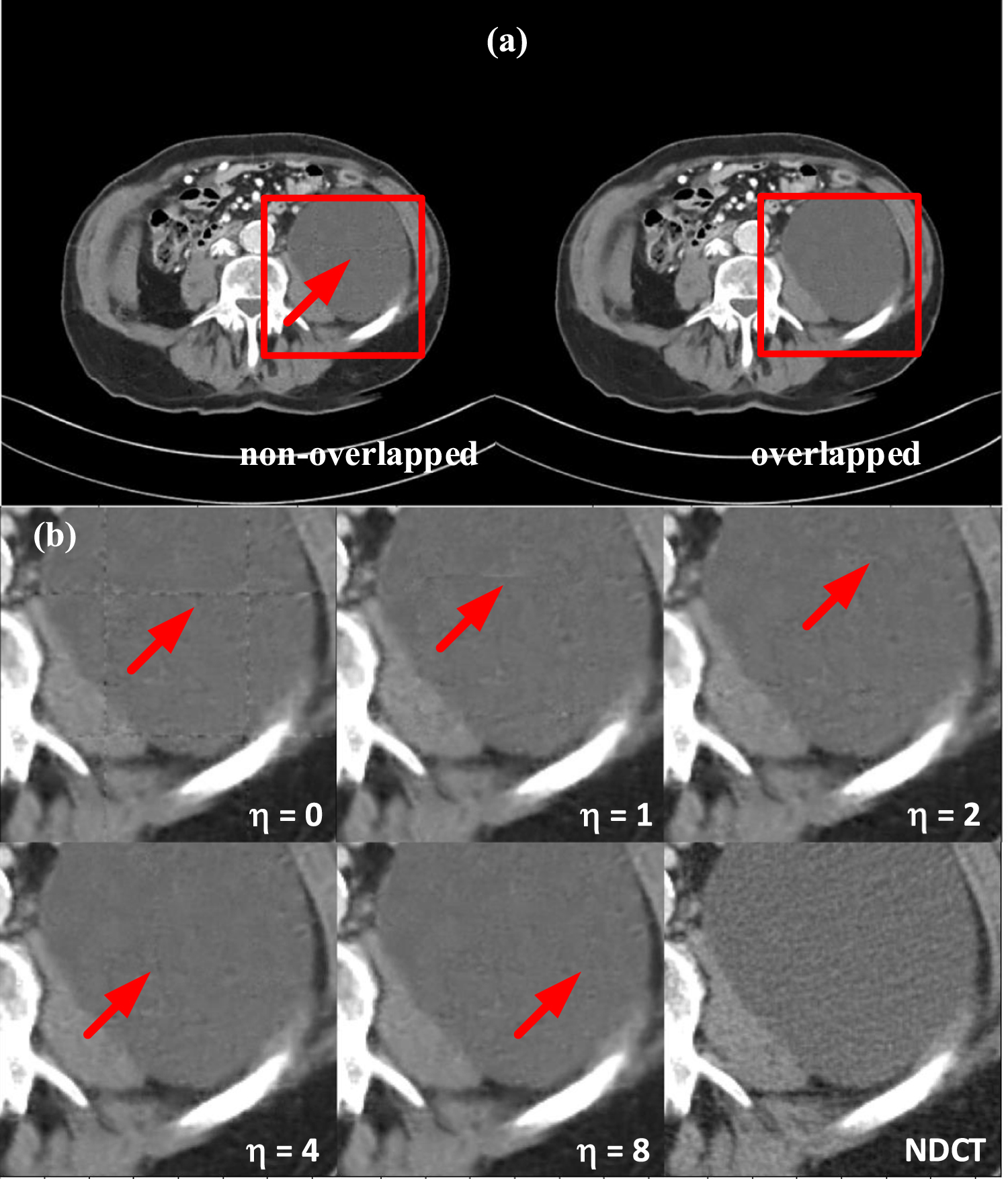
Eliminating boundary artifacts. The overlapped inference is performed to eliminate boundary artifacts as shown in figure 8(a). From the ROIs in figure 8(b), we can see that the boundary artifacts are obvious when η is 0 or 1 but soon become hardly perceivable when η further increases. It is worth noting that as η varies, the boundary artifacts can appear in different regions because the size of the patches integrated in the final image is different. To further confirm the effectiveness of the overlapped inference, quantitative analysis on the patient L506 is also conducted. As seen from table 2, the SSIM and RMSE scores improve fast when η goes from 0 to 20 with a better performance on 16. The corresponding ratio of the extra computation over the authentic computation σ is calculated from equation (10):  . To sum up, the overlapped inference can sufficiently address the dense boundary artifacts.

Figure 8. (a) The denoised results of non-overlapped inference and overlapped inference. (b) The denoising results of different margin sizes on the ROIs indicated in (a).
Download figure:
Standard image High-resolution imageTable 2. The SSIM and RMSE scores improve with margin.
| Margin | 0 | 4 | 8 | 12 | 16 | 20 |
|---|---|---|---|---|---|---|
| SSIM ↑ | 0.9071 | 0.9098 | 0.9113 | 0.9116 | 0.9121 | 0.9120 |
| RMSE ↓ | 9.5671 | 9.1940 | 9.0890 | 9.0503 | 9.0233 | 9.0223 |
Visual interpretation. To reveal the latent learning behavior in the CTformer, we visualize the attention maps  in each layer. Specifically, we derive attention maps by averaging all grids of Att and resize it to the size of the original image. Then, the attention map is superimposed on the image with a transparency rate 0.4.
As shown in figure 9, the attention map in the first layer highlights the key object parts. Specifically, there are more attentions on the edges rather than the composition of key structures like bones. Moreover, there are scattered dotted attentions on the protruding texture in the original image. For the attention map in the second layer, it basically resembles the pattern in the first attention, but sparser and less focused on the structures. Next, the pattern in the third layer becomes semantically implicit. Finally, the attention in the fourth layer tends to ignore the edges of objects and emphasize the content where noise is concentrated.

Figure 9. The attention maps over different input slices on specific positions.
Download figure:
Standard image High-resolution imageSince attentions in different layers focus on different structures, we construct an explanatory graph to illustrate the flow of attention across various layers. In our experiments, the object nodes are represented by the pixel coordinates of the image. We select the top 60 activations in the attention maps as nodes using TopK/LM selection and identify the highest activation under each node's influence. By applying the proposed method, the whole TopK and LM graph are obtained in figures 10 and 11, respectively.

Figure 10. TopK method for extraction of high activations and the corresponding attention graph.
Download figure:
Standard image High-resolution image
Figure 11. Local maximum method for extraction of peak activations and the corresponding attention graph.
Download figure:
Standard image High-resolution imageFrom the TopK graph in figure 10, it can be seen that the attention flows across different testing slices have very similar patterns. First, from the first to the second layer, the attentions on the edges still favor other edges in the next layer as indicated by the white circle in figure 10. Second, most high activations from the second layer move to the top area of the third layer in a latent manner. Last, the top attentions in the third layer then spread across the noisy area in the fourth layer. While the TopK graph identifies the flow of the top activations, the LM graph illustrates that of the local protuberant objects. As shown in figure 11, the attention graphs of different slices using LM are also analogous. Compared to TopK graph, one principal distinction in the LM graph is that groups of local maximum activations tend to implicitly concentrate on the same point in the next layer. The white circles in figure 11 illustrate some concurrent points. Therefore, by inspecting the two attention graphs, the dynamic flow can be clearly followed. We can figure out how the object parts are co-activated and thus go through similar level of noise reduction.
In summary, the latent learning behavior of the CTformer can be visually interpreted statically and dynamically. This makes the proposed model more transparent and reliable for diagnostic decisions.
5. Ablation study
In this part, comparative experiments are conducted to study the impact of the T2TD block, the cyclic shift operation and the number of the intermediate transformer blocks.
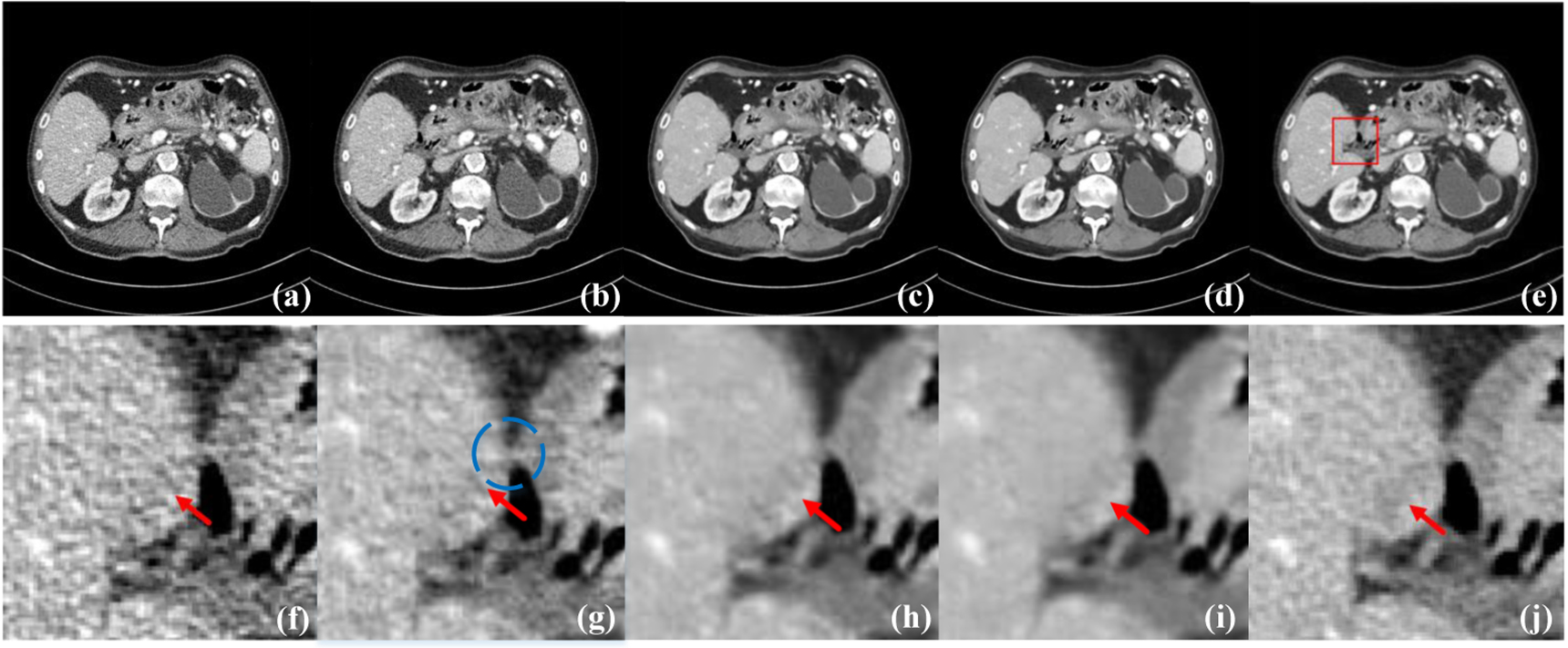
Impact of T2TD block. T2TD blocks are used in the CTformer to enhance the feature integration in the tokenization stage. Compared to fixed-region tokenization, the tokens in T2TD blocks are extracted from various regions of the original images. To verify the effectiveness of this part, a Sole-ViT model without the T2TD module is designed. We only adopt a sole convolution in the tokenization stage with a filter size of 8 and a stride of 8. Then five layers of transformer with an embedding size of 256 are applied for feature extraction and denoising. 256 rather than 64 embedding size is used because the model size and MACs are close to our model as shown in 3. Finally, a detokenization with deconvolution is employed to transform the tokens back to desired image domain. By investigating the conjunction area inside the blue circle in figure 12(g), we can see that Sole-ViT brings in extra blotchy tissues. Meanwhile, results in table 3 show that CTformer has better scores than Sole-ViT with a margin of 0.0235 on SSIM and 3.3362 on RMSE.

Figure 12. The performance of CTformer on case L506 with lesion No. 576. (a) LDCT, (b) Solve-ViT (c) CTformer without cyclic shift, (d) CTformer, and (e) NDCT. (f)–(j) are the corresponding magnified ROIs from (a)–(e).
Download figure:
Standard image High-resolution imageTable 3. Quantitative evaluation results of the Sole-ViT, the CTformer(W/oCS), and the CTformers with different number of transformer blocks.
| Method | TB | #param. | MACs | SSIM ↑ | RMSE ↓ |
|---|---|---|---|---|---|
| Sole-ViT | 1 | 2.92 M | 0.24 G | 0.8886 | 12.3595 |
| CTformer (W/oCS) | 1 | 1.45 M | 0.86 G | 0.9095 | 9.1570 |
| CTformer | 1 | 1.45 M | 0.86 G | 0.9121 | 9.0233 |
| CTformer | 2 | 1.48 M | 0.87 G | 0.9115 | 9.0303 |
| CTformer | 4 | 1.55 M | 0.91 G | 0.9108 | 9.1285 |
| CTformer | 8 | 1.68 M | 0.98 G | 0.9115 | 9.0841 |
Impact of cyclic shift. In this work, the cyclic shift is performed in the T2TD blocks to enhance the perceptual fields of our model. Figure 12 shows that CTformer with cyclic shift enjoys more spatial smoothness compared to the CTformer without cyclic shift. The latter introduces some additional noise components. Quantitative results from table 3 also confirm the effectiveness of cyclic shift in improving the SSIM and RMSE of the model by 0.0026 and 0.1337, respectively.
Impact of block number. In terms of the number of intermediate transformer blocks, we evaluate the CTformer with 1, 2, 4, and 8 blocks to identify the influence. When the block number grows, the network goes deeper. The computational cost increases slowly, but the actual training time climbs up dramatically. However, table 3 indicates that the CTformer with only one block yields the best performance over the ones with more blocks.
6. Discussion
Results on Mayo data showed that CTformer can effectively denoise 2D LDCT image. However, in clinical applications, real data is often acquired in 3D format, which implies the significance of 3D LDCT denoising task. Definitely, 3D LDCT denoising can be achieved by directly applying 2D denoising model slice by slice. However, in this way, the cross-slice spatial information are lost, which will probably lead to structural inconsistency in the synthesized images. Therefore, developing the corresponding 3D models for 3D LDCT is also a significant task. One simple way is to use the so-called 2.5D strategy. We can compute the averaged inputs and ground-truths of two consecutive slices to train the 2D transformer. Meanwhile, the CTformer can be extended to a 3D model by making some changes to the Tokenization/Detokenization module. Specifically, in the Tokenization module, instead of mapping 2D patches to 2D token sequences, we can map the 3D patches to 2D sequences. For example, a single tokenization area (3D block) can be unrolled into a sequence to represent a token. The Detokenization module simply takes the opposite operation while all other modules of the CTformer remain unchanged. Compared to 2D model, the 3D model should be able to exploit more of the spatial information, e.g. keeping more structural consistency across slices. Nevertheless, it demands more GPU memory and more data for training in practice.
7. Conclusion
In this paper, we have proposed a novel convolution-free transformer empowered by dilated tokenization and cyclic shift for LDCT denoising, which is referred to as the CTformer. To the best of our knowledge, the proposed CTformer is the first pure transformer model for LDCT denoising. Also, we have developed the interpretation methods for the proposed CTformer to decode its hidden behavior. Moreover, we have employed the overlapped inference to address the boundary artifacts that are common in an encoder-decoder model. Experimental results have demonstrated that the CTformer outperforms its competitors in terms of the denoising performance and model efficiency. However, the denoised images potentially suffer from certain level of oversmoothness, which will compromise the diagnostic value. In the future, we will incorporate perceptual and adversarial losses in the model to further refine the image textures and translate the CTformer into other medical denoising problems.
Data availability statement
The data that support the findings of this study are openly available at the following URL/DOI: https://doi.org/https://www.aapm.org/GrandChallenge/LowDoseCT/. Data will be available from 1 August 2016.
Ethical statement
This research study was conducted retrospectively using human subject data made available in open access by the Mayo clinic. Ethical approval was not required as confirmed by the license attached with the open-access data.
Appendix
Multiple doses study The performance of the CTformer on multiple low-dose levels is also studied in this section. To simulate the realistic clinical environment, we first obtain the projection datasets of Radon transform from the Manifold and Graph Integrative Convolutional Network (MAGIC) (Xia et al 2021b). Then, the CT images of different dosages are synthesized by adding Poisson and electronic noise to the projections. The geometry of the scan is listed as follows: The number of detector units is 1024, with a unit pitch of 1.2854 mm. The distance from the x-ray source to the isocenter of image is 595 mm. The distance from the detector to the source is 1085.6 mm. The size of the image pixel is 0.6641 mm. With the obtained sinograms, other dose levels are synthesized by adding different Poisson noises to the noise-free projections. Mathematically, the noisy projections are obtained by the following formula:

where I0 represents the x-ray intensity.  is the noise-free sinogram and
  is the variance in the normal distribution. In our experiment, the electronic noise variance is set to 10 according to Niu et al (2014), Xia et al (2021a). Then, the noisy CT images are reconstructed using filtered back projection algorithm in MAGIC.
As shown in table A1, different x-ray intensity levels are used to generate different dose images. Then, CTformer with patch embedding of 256 is used to denoise the images. Generally, stronger noise in LDCT will pose more challenge for the denoising model. Nevertheless, results in figure A1 show that the CTformer is effective in noise removal and structural preservation throughout a range of dose levels. Quantitative results in table A1 also confirm the efficacy of the CTformer in the denoising of multiple level LDCT.

Figure A1. Representative results of CTformer on CT images of different dose levels.
Download figure:
Standard image High-resolution image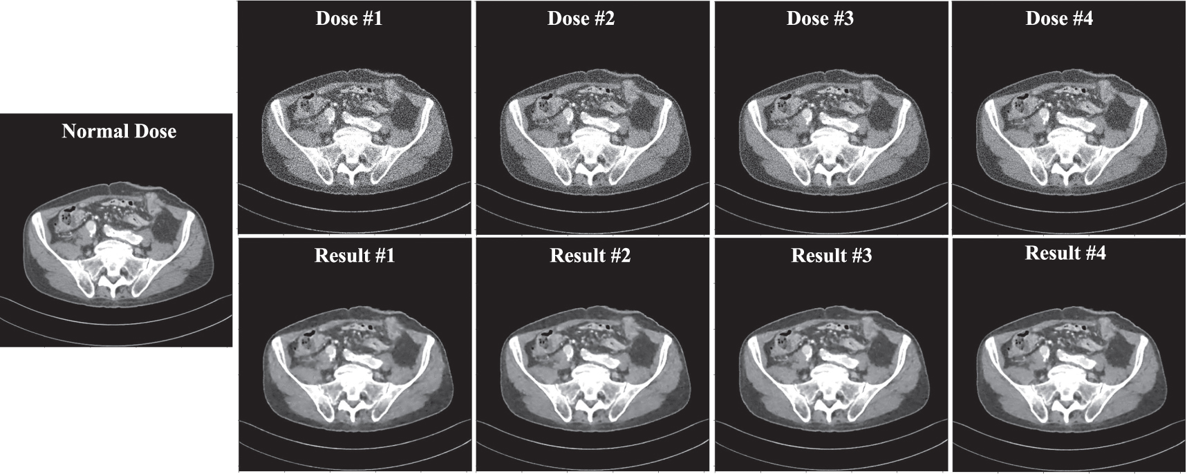
Table A1. Quantitative results before/after the CTformer is performed on the multiple dose level LDCT.
| Dose | x-ray intensity | SSIM (before) | SSIM (after) | RMSE (before) | RMSE (after) |
|---|---|---|---|---|---|
| Dose #1 | 5e4 | 0.7201 | 0.8744 | 39.9146 | 11.7762 |
| Dose #2 | 7.5e4 | 0.7615 | 0.8989 | 29.0673 | 9.8999 |
| Dose #3 | 1e5 | 0.7882 | 0.9126 | 24.0138 | 9.0970 |
| Dose #4 | 2.5e5 | 0.8078 | 0.9197 | 20.9208 | 8.5370 |