
Abstract
Objective. Presently electron beam treatments are delivered using dedicated applicators. An alternative is the usage of the already installed photon multileaf collimator (pMLC) enabling efficient electron treatments. Currently, the commissioning of beam models is a manual and time-consuming process. In this work an auto-commissioning procedure for the Monte Carlo (MC) beam model part representing the beam above the pMLC is developed for TrueBeam systems with electron energies from 6 to 22 MeV. Approach. The analytical part of the electron beam model includes a main source representing the primary beam and a jaw source representing the head scatter contribution each consisting of an electron and a photon component, while MC radiation transport is performed for the pMLC. The auto-commissioning of this analytical part relies on information pre-determined from MC simulations, in-air dose profiles and absolute dose measurements in water for different field sizes and source to surface distances (SSDs). For validation calculated and measured dose distributions in water were compared for different field sizes, SSDs and beam energies for eight TrueBeam systems. Furthermore, a sternum case in an anthropomorphic phantom was considered and calculated and measured dose distributions were compared at different SSDs. Main results. Instead of the manual commissioning taking up to several days of calculation time and several hours of user time, the auto-commissioning is carried out in a few minutes. Measured and calculated dose distributions agree generally within 3% of maximum dose or 2 mm. The gamma passing rates for the sternum case ranged from 96% to 99% (3% (global)/2 mm criteria, 10% threshold). Significance. The auto-commissioning procedure was successfully implemented and applied to eight TrueBeam systems. The newly developed user-friendly auto-commissioning procedure allows an efficient commissioning of an MC electron beam model and eases the usage of advanced electron radiotherapy utilizing the pMLC for beam shaping.
Export citation and abstract BibTeX RIS

Original content from this work may be used under the terms of the Creative Commons Attribution 4.0 licence. Any further distribution of this work must maintain attribution to the author(s) and the title of the work, journal citation and DOI.
1. Introduction
Over the last few decades, an enormous effort was made to replace patient-specific blocks in photon radiotherapy with a photon multileaf collimator (pMLC). Initially, the pMLC substantially improved treatment efficiency and safety (Brewster et al 1995, Boyer et al 2001). Along with such new hardware, expansions of new treatment planning capabilities like inverse treatment planning were accomplished. These further enabled the development of dynamic delivery techniques like intensity modulated radiotherapy (IMRT) or volumetric modulated arc therapy (VMAT), which both are current state-of-the-art delivery techniques in photon radiotherapy (Convery and Rosenbloom 1992, Bortfeld et al 1994, Yu 1995, Otto 2008). More recently new delivery techniques including even more degrees of freedom such as dynamic trajectory radiotherapy (DTRT) (Fix et al 2018, Guyer et al 2022) were proposed (Smyth et al 2019). However, a similar effort was not made for electron radiotherapy. Standard electron treatments are still applied using the cumbersome and inefficient standard or molded patient-specific cut-out placed in dedicated electron applicators for which limited planning features are available (Klein et al 2008). The usage of standard electron treatments needs effort in commissioning and maintenance for each energy-applicator combination and the fabrication of cut-outs including toxic materials (Fix et al 2013, Skinner et al 2019). Furthermore, combined photon and electron treatments have to be interrupted to mount and dismount the heavy add-on applicators (Henzen et al 2014b). In addition, treatment errors due to accidentally using a wrong cut-out are a potential risk (Mueller et al 2018a). All these issues negatively affect the workflow in clinical routine and make intensity and energy modulation of electron beams virtually unrealizable. Thus, the potential of electron radiotherapy is not yet utilized, although their sharp distal dose fall-off in tissue provides fundamentally different characteristics compared with photon beam dose distributions. This characteristic makes electron beams suitable for treatments of superficial targets. In research institutions the potential of electron beam dose characteristics was investigated by means of inverse planning based advanced techniques. These techniques include modulated electron radiotherapy (MERT) using either a few leaf electron collimator (Al-Yahya et al et al 2005, Al-Yahya et al 2007, Alexander et al 2010, Eldib et al 2013), a dedicated add-on electron MLC (Engel and Gauer 2009, Vatanen et al 2009, Gauer et al 2010, O'Shea et al 2011b, Jin et al 2014) or the pMLC (du Plessis et al 2006, Jin et al 2008, Klein et al 2008, Klein et al 2009, Salguero et al 2009, Salguero et al 2010, Mihaljevic et al 2011, Henzen et al 2014a, 2014c, Lloyd et al 2016, Kaluarachchi et al 2020). Using pMLC based collimation devices for electron beams offers great advantages with respect to the above-mentioned limitations for current standard electron treatments. The usage of the pMLC has the additional benefit that the pMLC is already part of the treatment unit head. Thus, no additional add-on hardware has to be mounted or dismounted, which improves safety, reduces workload for radiation therapy technologists and avoids gantry sag due to the weight of an electron beam add-on device. Using the pMLC for electron beams is also valuable for the treatment workflow, specifically for advanced treatment techniques such as MERT, mixed beam radiotherapy (MBRT) (Klein et al 2008, Surucu et al 2010, Ge and Faddegon 2011, Palma et al 2012, Renaud et al 2017, 2019, Heng et al 2021, Mueller et al 2022) or dynamic mixed beam radiotherapy (Mueller et al 2018b).
Using a Monte Carlo (MC) based beam model and dose calculation for predicting the dose distribution of electron beams in radiotherapy is well established and available in commercial products for standard electron beam applications (Cygler et al 2004, Cygler et al 2005, , Ding et al 2005, Ding et al 2006, , Pemler et al 2006, Popple et al 2006, Fragoso et al 2008, Edimo et al 2009, Ali et al 2011, Ojala et al 2016, Huang et al 2019, Snyder et al 2019). In order to apply electron beams with field sizes shaped by the pMLC, the currently used beam models in treatment planning systems for applicator-based electron beam delivery are not appropriate. Instead of the applicator, the pMLC has to be considered in the beam model. Furthermore, a commissioning procedure for such a beam model is an essential requirement for widespread use. Currently, such procedures are performed mainly manually and typically in an iterative manner including substantial computational resources and many user interactions (Leal et al 2004, Jin et al 2008, Klein et al 2008, Mihaljevic et al 2011, Henzen et al 2014c, Lloyd et al 2016, Mueller et al 2018a, Kaluarachchi et al 2020). An automated commissioning was presented by Henzen et al (2014c) applied for a single Clinac and a single TrueBeam system for different field sizes at a source to surface distance (SSD) of 70 cm. However, this commissioning procedure is limited to a sub-set of beam model parameters, which are not sufficient for a larger range of SSDs and TrueBeam systems. Therefore, manual commissioning steps have to be performed for the remaining beam model parameter. Hence, the currently applied approaches are time consuming meaning the commissioning takes up to several days. In addition, dedicated MC expertise as well as a detailed knowledge of the beam model are needed. In this work a fast (i.e. ∼ minutes) and user-friendly auto-commissioning process of the beam model part representing the beam above the pMLC was developed for TrueBeam systems (Varian Medical Systems, Palo Alto, CA) using the pMLC for shaping the electron fields and electron energies ranging from 6 to 22 MeV. This auto-commissioning was then validated for eight different TrueBeam systems.
2. Methods
The development of the proposed auto-commissioning procedure for the beam model part representing the beam above the pMLC consists of different parts illustrated in figure 1 and described in detail in this section. First the beam model itself including the sampling procedure is described (see section 2.1). Next information of the MC simulations performed using EGSnrc (see section 2.2.1) and simulations using the electron MC (eMC) algorithm eMC-2020 (see sections 2.2.2 and 2.5) are provided. These MC simulations include the pre-determined information to be performed only once, meaning the resulting data is used for all TrueBeam systems. Finally, the descriptions of necessary measurements of a specific TrueBeam system (see section 2.3) and the auto-commissioning (see section 2.4), which determines the tunable parameters of the beam model, are provided.

Figure 1. Overview of different parts of the proposed procedure. The arrows indicate which part provides input information for other parts in the procedure. (eMC-2020 refers to the electron MC algorithm described in section 2.5).
Download figure:
Standard image High-resolution image2.1. Electron beam model
In this section the beam model and the corresponding sampling procedure is described. A schematic view is depicted in figure 2.

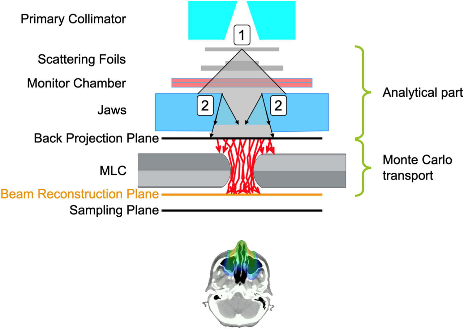
Figure 2. Schematic view of the proposed beam model and dose calculation algorithm. The beam model consists of a patient independent analytical part ([1] = main source and [2] = jaw source) followed by a patient specific Monte Carlo radiation transport layer. The beam model reconstructs the electron beam of a specific beam energy in the beam reconstruction plane starting from a sampling plane followed by a dedicated back projection algorithm to the back projection plane from where the Monte Carlo transport is applied. The particles are then provided for the dose calculation algorithm for which the electron Monte Carlo is used (see section 2.5).
Download figure:
Standard image High-resolution image2.1.1. Beam model
The beam model considered in this work is based on the beam model described in Henzen et al (2014c). The beam defining components of the accelerator are illustrated in figure 2, which are represented by the two sources in the analytical part and the pMLC as the patient specific component for which MC radiation transport is performed.
The primary electrons and bremsstrahlung photons are characterized by a main source with a focus f located closely to the scattering foil system in the linear accelerator head of a TrueBeam system. In addition, the main source (electrons and photons) is associated with a two-dimensional lateral Gaussian shaped intensity origin distribution with a standard deviation σf . To determine the initial direction of the source particle, a fluence distribution in a plane typically located at an SSD of 70 or 75 cm, referred to as sampling plane in figure 2, is related to this source. In addition, an electron and photon energy spectrum are assigned to the main source. The scattered electrons and photons of all components in the treatment head except the scattering foil are associated with the jaw source, which consists of four sub-sources linked to the four secondary collimator jaws. The secondary collimator jaws are set to a patient independent static field size of 15 × 35 cm2 for accelerators equipped with a Millennium 120 pMLC (M120), while this field size is reduced to 15 × 17 cm2 in the case where the high-definition pMLC (HDMLC) is used. These settings remain the same for all electron beam energies. Each sub-source defines a line source for electrons and photons similar to the line source defined in a previous publication for applicator-based electron radiotherapy (Fix et al 2013). The origin distribution is represented by a horizontal line on the inner side of the jaw for which the width corresponds to the jaw setting of the corresponding field size. Similar to the main source, a fluence distribution in the sampling plane is used to determine the initial direction of the source particle. Furthermore, an electron and photon energy spectrum are associated with the line source. Finally, a sampling procedure for the beam model is defined to provide a particle for the dose calculation algorithm in the beam reconstruction plane (figure 2).
2.1.2. Sampling procedure
The sampling procedure applied for the beam model reconstructs the radiation beam in the beam reconstruction plane (figure 2) and consists of the following steps:
- 1.Sample the sub-source.
- 2.Sample a point in the beam sampling plane from the two-dimensional fluence distribution for the sub-source determined in step 1.
- 3.Sample the energy from the energy distribution for the sub-source determined in step 1.
- 4.Determine the initial direction by connecting the point in the beam sampling plane (step 2) with a sampled point from the origin distribution for the sub-source determined in step 1.
- 5.In case of a photon particle, ray-tracing is applied to determine if the photon hits the jaws. In case the photon hits the jaws, the photon is rejected. Otherwise, the location in the back projection plane (figure 2) is determined by ray-tracing.
- 6.In case of an electron particle, the initial direction of the electron determined in step 4 is corrected in order to account for the in-air scatter along the path from the origin to the sampling plane. The correction values for the direction cosines u and v for the electron is sampled form a Gaussian distribution with an energy E dependent standard deviation σθ (E), which is determined using the Highland approximation for in-air scatter corrections (Lynch and Dahl 1991). At this stage the sampling of the starting point does not take into account the impact of the jaws. The impact of the jaws is corrected by back projecting the electrons to the plane of the jaws. This procedure was described in Fix et al (2010, 2013) except that in this work the Highland approximation for in-air scatter is used. With this procedure it is determined whether or not the electron passes through the opening of the jaws. The electron is rejected if it does not pass through the opening of the jaws. Otherwise, the electron is projected to the back projection plane.
- 7.For the non-rejected particle, MC radiation transport through the pMLC starts in the back projection plane downstream to the beam reconstruction plane. In case the particle or all potentially created secondary particles reach this plane, they are passed on to the dose calculation algorithm.
Thus, for the commissioning procedure of the proposed beam model representing the analytical part the following parameters have to be determined for the specific electron beam energy: for the main electron and photon source the focus position, the focus size, the fluence distribution and the energy spectrum in the sampling plane and for the jaw source or more specifically for each of the four electron and photon sub-sources the origin distribution as well as the fluence distribution and energy spectrum in the sampling plane. In addition, the weight of each individual sub-source has to be determined.
2.2. Pre-determined MC simulations
In this work, the auto-commissioning of the beam model for a specific treatment unit of a TrueBeam system is performed based on a sampling plane at an SSD of 70 or 75 cm, which does not have to coincide with the beam reconstruction plane expected to be closer to the pMLC. The secondary collimator jaws are set to a static field of 15 × 35 cm2 or 15 × 17 cm2 when the TrueBeam system is equipped with the M120 or the HDMLC, respectively. For these settings pre-calculated information is determined by MC simulations for a treatment unit in general, that is independent of a specific linear accelerator instance, and described in the following sections.
2.2.1. MC simulation using EGSnrc
This part consists of full MC simulations using EGSnrc as the transport code (version 2020) (Kawrakow and Rogers 2002). For these simulations BEAMnrc (Rogers et al 1995) was applied to model the beam defining components including the primary collimator, the scattering foil system, the monitor chamber, the secondary collimator jaws and the reticle for the different electron beam energies. The input is based on confidential information from Varian Medical System (Palo Alto, CA) for Clinac linear accelerators together with physical measurements on scattering foils performed, which is considered to be suitable to represent a TrueBeam system for the purpose of this work and supported by the work of Lloyd et al (2015). During these simulations, phase space files in the sampling planes at SSD = 70 and 75 cm for the maximal field size possible (40 × 40 cm2), and the field size used for the beam model were generated. These phase space files were analyzed in order to determine radiation beam characteristics. One aspect of the phase space file analyses was the particle fluence referred as fluence in the following. For this purpose, all particles (electrons and photons) from the scattering foil system were initially assigned to the main source. However, if the particle interacts in one of the secondary collimator jaws, they were re-assigned to the jaw source of the corresponding collimator jaw. For the purpose of particle assignment to a source, the particle history was scored during the MC simulation and accordingly stored in the phase space file. During the evaluation of the phase space file, the particles can then be sorted according to the different sources considered. This is especially important as the contributions of the different sources cannot be separated in the measurement data, but are needed for the auto-commissioning.
In addition to the fluence in the sampling plane, also the origin distribution for the jaw source was analyzed based on the phase space files. As mentioned above, the origin distribution for each jaw sub-source is a line located on the beam shaping surface of each jaw. While the true origin distribution covers the complete surface along the beam direction, this distribution is not homogeneous and the line determined represents the average value of the extracted distribution from the phase space files.
Apart from the determination of the fluence also the energy spectrum of each photon source (main and jaw) was extracted from the phase space file for each electron beam energy.
Finally, the depth dose curve for the jaw sources was calculated by performing MC simulations using DOSXYZnrc with the corresponding particles from the phase space files as input. All these simulations were performed for each electron beam energy considered, namely 6, 9, 12, 15, 16, 18, 20 and 22 MeV.
In summary, this part provides the following input to the eMC-2020 simulations (see section 2.2.2), the auto-commissioning (see section 2.4) as well as the beam model (see figure 1):
- Electron fluence of the jaw source used in the eMC-2020 simulations, the auto-commissioning as well as the beam model.
- Photon fluence of the main and jaw source used in the eMC-2020 simulations, the auto-commissioning as well as the beam model.
- Origin distribution of the jaw source used in the eMC-2020 simulations and the beam model.
- Photon energy distributions of the main and jaw source used in the eMC-2020 simulations and the beam model.
- Depth dose curve in water of the jaw source used in the auto-commissioning.
2.2.2. Simulation using eMC-2020
In addition to the MC simulation described in the previous section, additional depth dose calculations are needed for the auto-commissioning using the identical dose calculation algorithm as for which the beam model is commissioned. In this study the electron MC (eMC) algorithm eMC-2020 (see section 2.5) is used. This guarantees the reproducibility of calculated dose distributions when using the commissioned beam model in conjunction with eMC-2020. In total four different sets of depth dose curves were calculated, namely for:
- Mono-energetic electrons of the main electron source.
- Mono-energetic electrons of the jaw electron source.
- The main photon source using the energy spectrum from the EGSnrc simulation.
- The jaw photon source using the energy spectrum form the EGSnrc simulation.
Thereby for the main sources the calculations were performed for different locations of the focus f of the main source at distances of 6, 8, 10, 12 and 14 cm from the upper surface of the photon bremsstrahlung target being the typically used origin of the central beam axis. In addition, for each focus position f different σf values of 0.0, 0.5, 1.0, 1.5 and 2.0 cm were considered. For all the four above mentioned sets of depth dose calculations the following situations were included: field sizes of 15 × 35 cm2 and 15 × 17 cm2, SSD1 = sampling plane (70 or 75 cm) and SSD2 = 90 cm, pMLC shaped field sizes of 2 × 2 cm2, 5 × 5 cm2 and fully retracted pMLC leaves.
2.3. Measurements
In order to perform the auto-commissioning a set of dose measurements are needed to determine the tuning parameters of the beam model. For the proposed auto-commissioning procedure, the following set of measurements for each electron beam energy are required:
- Relative in-air dose profiles in crossline and inline directions with the pMLC fully retracted for a field size of 40 × 40 cm2 at SSD1.
- Depth dose curves in water at SSD1 and SSD2 in units of cGy/MU with the pMLC fully retracted and field sizes of either 15 × 35 cm2 or 15 × 17 cm2 depending on the pMLC type available.
- Depth dose curves in water at SSD1 in units of cGy/MU and pMLC shaped field sizes of 5 × 5 cm2 and 2 × 2 cm2.
The complete set of commissioning measurements were performed for in total eight TrueBeam systems with seven TrueBeam systems equipped with a M120 and one TrueBeam system equipped with an HDMLC. Thereby, the electron beam energy ranges from 6 to 22 MeV. Table 1 summarizes the data available.
Table 1. Overview of the TrueBeam systems including the set of electron beam energies, for which a complete commissioning data set together with additional validation measurements were available. The last column provides information of the water tank and detector (field & reference detector) equipment used for the measurements (mD = microDiamond; SF = Semiflex 31010; D = diode TW60017; E = EDGE-Detector).
| TB-System | 6 MeV | 9 MeV | 12 MeV | 15 MeV | 16 MeV | 18 MeV | 20 MeV | 22 MeV | Measurement equipment used |
|---|---|---|---|---|---|---|---|---|---|
| Millennium-1 | X | X | X | X | X | X | MP3 mD & SF | ||
| Millennium-2 | X | X | X | X | X | X | BEAMSCAN mD & SF | ||
| Millennium-3 | X | X | X | X | X | X | BEAMSCAN mD & SF | ||
| Millennium-4 | X | X | X | X | X | MP3 mD & SF | |||
| Millennium-5 | X | X | X | X | X | MP3 mD & SF | |||
| Millennium-6 | X | X | X | X | X | BEAMSCAN mD & SF | |||
| Millennium-7 | X | X | X | X | 3D Scanner D & E | ||||
| HDMLC-1 | X | X | X | X | X | BEAMSCAN mD & SF |
These measurements were performed using a MP3, a BEAMSCAN (both PTW Freiburg, Germany) or a 3D Scanner (Sun Nuclear, Melbourne, FL) water tank. For the two PTW water tanks a microDiamond and a Semiflex 31010 (both PTW, Freiburg, Germany) were used as field detector and reference detector, respectively. In case of the 3D scanner water tank a diode detector TW60017 (PTW, Freiburg, Germany) and an EDGE-Detector (Sun Nuclear, Melbourne, FL) was used as field detector and reference detector, respectively.
2.4. Auto-commissioning
The auto-commissioning procedure is illustrated in figure 3:
- 1.The first step in the auto-commissioning part is to construct a two-dimensional fluence distribution for the main electron source. For this purpose, the measured in-air profiles in crossline and inline direction at SSD1 using a 40 × 40 cm2 field size (at iso-center) are used. The corresponding contribution from electrons from the secondary collimator jaws as determined by MC simulations using EGSnrc (see figure 2) are subtracted from these measured in-air profiles. This results in measured fluence profiles for the main electron source px and py in crossline and inline direction. The two-dimensional fluence distribution
 for the electrons of the main source is then determined by the following equation:For the photons of the main source the fluence distribution as determined by the EGSnrc MC simulation is used.
 - 2.In the next step, the measured depth dose contribution from the main source (electrons and photons) at SSD1 is extracted. This is done by subtracting the pre-calculated jaw source depth dose curve using EGSnrc MC simulations from the measured depth dose curve. In this step the depth dose contribution from the jaws is multiplied by a jaw-fraction factor with values of 1%, 2%, 4%, 6%, 8% or 10% of the measured depth dose curve around the maximum dose.
- 3.Then the measured depth dose contribution from the main source is de-convolved with the corresponding pre-calculated depth dose curves for mono-energetic electrons and the photon depth dose curve for the main source. This results in the energy spectrum of the electrons of the main source as well as the source weight of the photons of the main source.
- 4.Now the contribution to the depth dose curve in water of the electrons and photons from the main source can be calculated at SSD1.
- 5.The depth dose curve contribution determined in step 4 is now subtracted from the measured depth dose curve leading to the measured depth dose associated with the jaw source.
- 6.Similar to step 3 the resulting measured depth dose curve from step 5 is de-convolved with the corresponding pre-calculated depth dose curves for mono-energetic electrons and the photon depth dose curve for the jaw source. In addition, the source weight of the photons of the jaw source is obtained.
- 7.Now all parameters are determined in order to calculate the total depth dose curve in water at SSD2 with the pMLC fully retracted.
- 8.Steps 3 to 7 are repeated for each location of the focus f of the main source. These depth dose curves as a function of the focus f are now compared with the corresponding measured depth dose curve at SSD2. Interpolation of the focus location f to match this measured depth dose curve is performed to determine the final focus f of the main source for a given σf and jaw-fraction.
- 9.Now all steps from 3 to 6 are repeated for each value of σf . Then the depth dose curves in water at SSD1 for an pMLC shaped field size of 2 × 2 cm2 are calculated. These depth dose curves as a function of σf are now compared with the corresponding measured depth dose curve. Interpolation of σf to match this measured depth dose curve is performed to determine the final value for σf of the main source for a given jaw-fraction.
- 10.Next all steps from 2 to 9 are repeated for each value of jaw-fraction and the depth dose curves in water at SSD1 for an pMLC shaped field size of 5 × 5 cm2 are calculated. These depth dose curves as a function of jaw-fraction are now compared with the corresponding measured depth dose curve. Interpolation of the jaw-fraction to match this measured depth dose curve is performed to determine the final value for the jaw-fraction.


Figure 3. Flow chart of the auto-commissioning procedure. The different steps (1 to 10) are described in the text. The upper part (dark grey) in the rectangles illustrates what is performed in the step, while the lower part indicates the input used for the step. The source of the input data shown is additionally indicated by different colours: yellow refers to measured data, red refers to pre-calculated data based in EGSnrc Monte Carlo simulations, green refers to pre-calculated data based on eMC-2020 (see section 2.5) and blue indicates specific settings for the MLC and SSD as well as for the used beam model parameters in the step. (DD = depth dose; f = focus position of the main source; σf = focus size of the main source; main and jaw refer to the main source and jaw source, respectively).
Download figure:
Standard image High-resolution imageAfter the completion of the ten steps all parameters of the beam model are determined and the commissioning procedure is fully completed.
During the auto-commissioning the focus position f and the standard deviation σf of the main source associated with the spot size are determined in step 8 and 9. Both parameters are determined independently from each other. This is possible as these parameters are established by means of different measurements and the depth dose curve for the field size with fully retracted pMLC is virtually independent on the spot size, hence the corresponding measured depth dose curve at SSD = 90 cm can be used to determine the position of the focus. Given the position of the focus the depth dose curve for the pMLC shaped field size of 2 × 2 cm2 is then used to determine the value for σf .
2.5. Dose calculation
The fully commissioned beam model provides the particles in the beam reconstruction plane for the dose calculation algorithm (see figure 2). The dose calculation performed in this work is based on the eMC algorithm for both pre-determined MC simulations and validation (Neuenschwander and Born 1992, Fix et al 2013). Compared to the previously used version of this dose calculation algorithm, a new version was used for this study, referred to as eMC-2020, which includes improvements recently developed for this work. This version is based on local simulations performed with the more recent EGSnrc version 2020 (Kawrakow and Rogers 2002). In this context not only the program language was changed from Mortran to C++ for the simulation framework using the advanced application in egs++ to generate the database for eMC-2020 in the local simulation, but also improvements in the macro simulation were included. Mainly the following improvements were implemented in the version of eMC-2020 used in this work, for which some more detailed information about these improvements is provided in the appendix:
- 1.The correlation between energy and direction of secondary particles was taken into account. Hence, the generation of the database was modified to score the data needed for such a correlated sampling.
- 2.The energy deposition of the primary electron was modified. The new version takes the small build-up effect occurring in the spheres into account and thus improves the energy deposition distribution of the local simulation in the macro step compared with the previous versions.
- 3.Lung with density 0.1 g cm−3 (lung light) was included in the database as an additional sampling material between air and lung with density 0.3 g cm−3.
- 4.Dedicated and efficient air transport.
The statistical uncertainty of the MC calculated dose distributions was less than 1% (one std. dev.).
2.6. Validation
As a first test of the completely commissioned beam model calculations of the dose distributions for those situations used during the commissioning are performed in order to demonstrate that the beam is able to reproduce the measured dose distributions as expected by design. Secondly and to validate the commissioned beam model, calculated and measured dose distributions in water were compared for different pMLC shaped field sizes (2 × 2, 5 × 5, 10 × 10 cm2) at SSDs ranging from 70 to 100 cm for electron beam energies ranging from 6 to 22 MeV.
Finally, a clinically realistic sternum case is considered as validation for the commissioned beam model. For this purpose, an Alderson anthropomorphic phantom is used and a CT scan from the chest part including the sternum is performed. The contours of the clinical target volume (CTV), the planning target volume (PTV) and structures of organs at risk, that is lungs and heart, from a clinical case are converted to the Alderson phantom to obtain a realistic situation. A dose of 30 Gy in 10 fraction was prescribed to the median dose of the PTV. Electron beams were manually setup utilizing a 22 MeV electron beam for this sternum case at two different SSDs of 75 and 96 cm. Applying an SSD = 75 cm demonstrates a short but still realistic SSD, while an SSD = 96 cm demonstrates a use case in which the iso-center corresponds with the iso-center used for image guided setup. Since due to in-air scatter of the electrons degrades the penumbra of the electron beam, reduced SSDs are advantageous (Klein et al 2008). The dose distributions for the pMLC shaped electron field are calculated using the commissioned beam model together with the eMC-2020 dose calculation algorithm at both SSDs. During dose delivery in the developer mode of a TrueBeam equipped with a M120 pMLC, dose distributions using radiochromic films were measured in two transversal planes of the Alderson phantom per SSD. For this purpose, the scanned films were corrected for lateral scanner response artefacts (Lewis and Chan 2015). A triple channel calibration was used to convert the scanned values to absolute dose along with the one-scan protocol (Micke et al 2011, Lewis et al 2012). The red color channel was used for the comparison of the four measured dose distributions with the corresponding calculated dose distributions by means of gamma passing rates. Gamma criteria of 3% (global) and 2 mm, 2% (global) and 2 mm as well as 1% (global) and 2 mm each with a threshold of 10% were used.
3. Results
3.1. Commissioning
The auto-commissioning was successfully implemented and applied for all available energies of the eight TrueBeam systems. Instead of the manual commissioning taking up to several days of calculation time and several hours of user time, the auto-commissioning is carried out in a few minutes for a single TrueBeam system.
Initially, all of the collected measurement data were reviewed. The analysis of measured lateral dose profiles at a depth of 1 cm in water in crossline and inline directions identified a systematic lateral offset of the dose profiles in inline direction of all the TrueBeam systems considered in this work. This lateral offset is different for different electron beam energies and most pronounced for high electron beam energies and an offset of up to about 2 mm at SSD = 90 cm was determined and is included optionally in the auto-commissioning process.
The first step in the auto-commissioning part is the construction of a two-dimensional fluence distribution for the main electron source and figure 4 shows examples of such measurements and fluence profiles along with the resulting two-dimensional fluence distributions for two different electron beam energies. Thereby the measured fluence distributions were normalized to one on the central axis.

Figure 4. Measured crossline in-air profiles in the sampling plane for two different beam energies are shown on the left together with the fluence for the electrons from the jaw source as determined by BEAMnrc MC simulations and the fluence distribution of the main electron source determined as the difference between the measured and the electron fluence from the jaws. The colour coded two-dimensional fluence distribution for the main electron source for these beam energies constructed based on the in-air measured profiles are shown on the right. These fluence distributions are used in the sampling process of the beam model. Data shown for the Millennium-1 system.
Download figure:
Standard image High-resolution imageDuring the auto-commissioning the focus position f and the standard deviation σf of the main source associated with the spot size are determined which is illustrated in figure 5. Both parameters are determined independently from each other. The depth dose curves at SSD = 70 cm with the MLC fully retracted match measurements within 1% for all settings of f, as expected. As illustrated in figure 5 there is a strong sensitivity of the output for the different settings of σf at the field size of 2 × 2 cm2, which is also increasing for increasing electron beam energy. The resulting depth dose curves by means of interpolation is shown to match the corresponding measurements.

Figure 5. Illustration of the determination of the position of the focus f and the sigma σf of the main source as described in the auto-commissioning part (see section 2.4.) for two electron beam energies. The tuning process is designed to match depth dose curves at SSD = 70 cm (used as sampling plane in this case). To also match the measured depth dose curve at SSD = 90 cm the used focus position is interpolated. Applying the final value of the focus position, the measured depth dose curve for the field size of 2 × 2 cm2 (at iso-center) is matched with calculated depth dose by interpolation of σf . Data shown for the Millennium-3 system.
Download figure:
Standard image High-resolution imageTable 2 presents the resulting final values for the tuning parameters of the locations of the focus f, the sigma of the Gaussian shaped intensity distribution σf as well as the jaw-fraction for the different electron beam energies for the TrueBeam systems equipped with the M120 pMLC.
Table 2. Overview of the resulting electron beam model parameter focus f, sigma σf and jaw-fraction per electron beam energy of the auto-commissioning part for all TrueBeam system equipped with the Millennium 120 pMLC. Note, that for 16 and 20 MeV only one system was available.
| Tuning Parameter | 6 MeV | 9 MeV | 12 MeV | 15 MeV | 16 MeV | 18 MeV | 20 MeV | 22 MeV |
|---|---|---|---|---|---|---|---|---|
| Focus f [cm] mean (min, max) | 8.5 (7.2, 9.8) | 8.0 (7.0, 8.8) | 9.4 (8.8, 9.9) | 8.4 (8.0, 8.8) | 8.2 | 8.1 (7.7, 8.6) | 8.5 | 8.3 (8.1, 8.5) |
| Sigma σf [cm] mean (min, max) | 1.26 (1.14, 1.40) | 0.63 (0.59, 0.69) | 0.52 (0.49, 0.57) | 0.50 (0.48, 0.55) | 0.46 | 0.45 (0.42, 0.48) | 0.44 | 0.42 (0.41, 0.44) |
| Jaw-fraction [%] mean (min, max) | 4.1 (2.8, 5.1) | 6.8 (6.3, 7.4) | 6.1 (5.6, 6.7) | 5.2 (4.9, 5.7) | 5.4 | 5.0 (4.4, 5.9) | 5.2 | 5.2 (5.0, 5.4) |
Over all electron beam energies and TrueBeam systems, the variation of the focus position is within 3.5 cm, with the largest system to system variation for the 6 MeV electron beam energy. Although the focus positions are around the locations of the electron scattering foil systems in the linear accelerator head, there is no clear correlation with the specific electron scattering foils used for the different electron beam energies. While there is no clear dependency for the focus position and jaw-fraction as a function of electron beam energy, the values for sigma decrease for increasing electron beam energy. In addition, the values for sigma are consistent and within 0.3 cm for the different TrueBeam systems and all electron beam energies and within 0.1 cm for the individual electron beam energies, except for the 6 MeV electron beam energy. The value for σf as well as its variation of within 0.25 cm for the 6 MeV beam is substantially larger compared to the remaining electron beam energies and might be due to the increase of in-air scatter at the low electron energy level. The corresponding values for the TrueBeam system equipped with the HDMLC are shown in table 3.
Table 3. Overview of the resulting electron beam model parameter focus f, sigma σf and jaw-fraction per electron beam energy of the auto-commissioning part for the TrueBeam system equipped with the high-definition pMLC.
| Tuning parameter | 6 MeV | 9 MeV | 12 MeV | 16 MeV | 20 MeV |
|---|---|---|---|---|---|
| Focus f [cm] mean | 9.4 | 9.0 | 10.4 | 8.6 | 8.2 |
| Sigma σf [cm] mean | 1.27 | 0.69 | 0.55 | 0.49 | 0.41 |
| Jaw-fraction [%] mean | 1 | 6.1 | 8.1 | 7.1 | 6.2 |
3.2. Validation
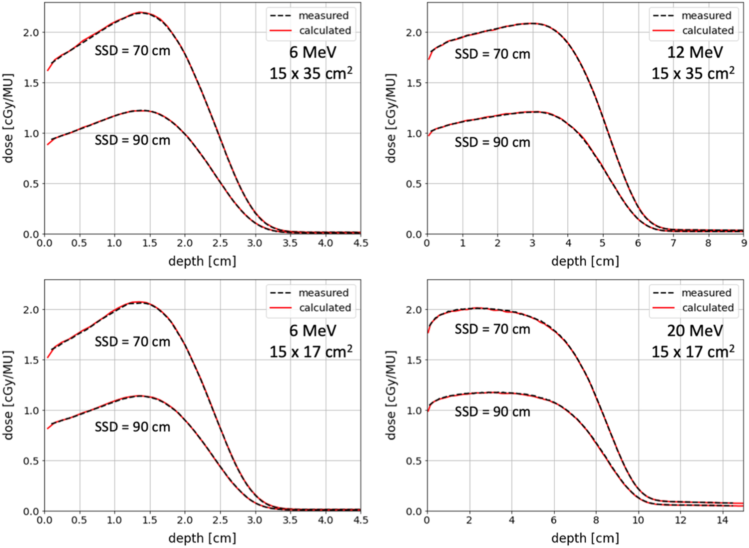
As a first validation of the completely commissioned beam model, calculations of the dose distributions for those situations used during the commission are performed and some results of this dosimetric comparison are shown in figure 6 in units of cGy/MU. Dose calculations in water using the fully commissioned beam model are able to match with the corresponding dose measurements generally within 1% for all situations considered.

Figure 6. Comparison of measured and calculated absolute depth dose curves in water for different beam energies and field sizes of 15 × 35 cm2 (upper row) and 15 × 17 cm2 (lower row) of TrueBeam systems equipped with the Millennium 120 pMLC and the high-definition pMLC, respectively. The sampling plane is located at SSD = 70 cm. The agreement between measured and calculated dose values is below 1%. Data shown for the Millennium-6 system (upper row) and for the HDMLC-1 system (lower row).
Download figure:
Standard image High-resolution imageThe next level of validation includes comparisons of measured and calculated dose distributions in water for situations that were not used during the auto-commissioning. Some validation results with depth dose curves and lateral dose profiles are exemplarily shown in figures 7 and 8 for TrueBeam systems equipped with the M120 and with the HDMLC, respectively.

Figure 7. Examples of validation results by means of comparisons of measured and calculated absolute dose distributions for different pMLC shaped field sizes (at iso-center), SSDs and electron beam energies for a TrueBeam system equipped with Millennium 120 pMLC. The shown lateral dose profiles are at a depth of 1 cm in water. Data shown for the Millennium-3 system.
Download figure:
Standard image High-resolution image
Figure 8. Examples of validation results by means of comparisons of measured and calculated absolute dose distributions for different pMLC shaped field sizes (at iso-center), SSDs and electron beam energies for TrueBeam systems equipped with high-definition pMLC. The shown lateral dose profiles are at a depth of 1 cm in water. Data shown for the HDMLC-1 system.
Download figure:
Standard image High-resolution imageNote that all these comparisons are performed in absolute dose units over a large range of field sizes and SSDs. Overall, measured and calculated dose distributions agree generally within 3% of maximum dose or 2 mm distance to agreement for all TrueBeam systems considered.
Finally, figure 9 presents an example validation of the comparison of film measured and calculated dose distributions for the sternum case by means of gamma analysis using 3% (global) and 2 mm criteria with a threshold of 10%. The gamma passing rates for the two situations were 99% (both films) for dose delivery at SSD = 96 cm and 99% and 96% for dose delivery at SSD = 75 cm considered using the criteria mentioned above. When using the 2% instead of the 3% criterion the gamma passing rate were 97% (both films) for dose delivery at SSD = 96 cm and 99% and 93% for dose delivery at SSD = 75 cm. Using the 1% instead of the 3% criterion the gamma passing rate were 95% and 92% for dose delivery at SSD = 96 cm and 96% and 89% for dose delivery at SSD = 75 cm.

Figure 9. The upper row shows the dose distribution (left) and the setup (right) for the sternum case of the Alderson phantom at an SSD of 75 cm. On the bottom left the iso-dose comparison of measured (thin lines) and calculated (thick lines) dose distributions for one slice at an SSD of 75 cm is depicted. The corresponding gamma distribution leads to 99% passing rate for 3% (global) and 2 mm criteria with a 10% threshold (lower right).
Download figure:
Standard image High-resolution image4. Discussion and conclusions
This work presents a newly developed auto-commissioning procedure of a MC based beam model for pMLC shaped electron beams applicable for TrueBeam systems equipped with a M120 or an HDMLC. The commissioned beam model reproduces the electron beam characteristics leading to accurate dose distributions for a large range of SSDs, field sizes and electron beam energies ranging from 6 to 22 MeV. This was demonstrated for in total eight TrueBeam systems. It is important to mention that the enormous computational effort spent in the pre-determined MC simulations (see section 2.2) has to be done only once and is then applicable for all consecutively performed auto-commissioning of other TrueBeam systems. Hence, the application of the proposed procedure does not require any specific MC expertise for the auto-commissioning. In addition, no information of the beam defining system of the treatment unit or knowledge on how to generate the pre-determined data is needed by the user. The obtained database allows the auto-commissioning of the individual TrueBeam systems in a few minutes, while previously applied manual procedures needed several days of computation time along with hours for the user. The resulting accuracy when compared with measurements corresponds at least to the level of agreement achieved for the manual procedure as shown by Mueller et al (2018a). Other studies achieved agreement between measured and calculated percentage depth dose curves and lateral dose profiles within mainly 2% or 2 mm (Jin et al 2008, Klein et al 2008, Mihaljevic et al 2011, Henzen et al 2014c, Lloyd et al 2016). However, these studies compared relative dose distributions for at most two SSDs, while in this study absolute dose distributions over a larger range of SSDs are considered. Some small remaining dose differences observed in the validation as for example shown in figures 6 and 7 might be due to uncertainties in the measurements such as setup uncertainties. In addition, also the beam model itself includes approximations and further improvements could reduce these remaining dose differences. Another advantage of the developed auto-commissioning procedure is that only two in-air dose profiles and four depth dose curves for the commissioning of one electron beam energy have to be acquired by the user with an additional lateral dose profile in order to determine the systematic lateral shift as discussed below. This is reduced compared to applicator-based electron radiotherapy, in which for each energy-applicator combination a set of dose measurements is needed (Cygler et al 2004, Ding et al 2006, Fix et al 2013, Huang et al 2019). For example, typically two to three days are needed to perform all commissioning measurements (including optional measurements) for a total of six electron beam energies for the electron MC algorithm in Eclipse (Varian Medical Systems, Palo Alto, CA). This can be reduced to one day for the commissioning measurements (including optional measurements) when using the proposed auto-commissioning.
When evaluating the different sets of measurements, a systematic shift of the lateral dose profiles in inline direction was observed. The larger the electron beam energy, the larger was the shift in the dose distribution reaching about 2 mm for the largest electron beam energy of 22 MeV considered in this work. This offset can be determined by means of a dose measurement and included optionally in the auto-commissioning process by either providing a value of this offset by the user or by providing a lateral dose profile acquired as described in the following. First the detector has to be aligned to the central beam axis using a 5 × 5 cm2 pMLC shaped field of a photon beam, assuming a centered beam alignment for photon beams. Note that this alignment procedure should also be used for the commissioning and validation measurements in order to avoid a misalignment due to the lateral offset in electron beams. Using this aligned detector position, the lateral dose profile in water in inline direction for a 5 × 5 cm2 pMLC shaped field is measured at a depth of 1 cm in water at SSD = 90 cm. Since the pMLC for a collimator angle of 0° is not symmetric in the inline direction (bottle shaped pMLC leaves), a collimator rotation of 90° or 270° is suggested to be applied in order to shape the field by the rounded leaf ends of the pMLC. A lateral shift in inline direction can then be determined as the difference between the central beam axis and the center of the measured lateral dose profile. We hypothesize that the reason for such lateral shifts might be a combination of the impact of the fringe magnetic field from the bending magnet and a lateral offset of the focus location on the scattering foil (O'Shea et al 2011a). The auto-commissioning procedure allows to include this shift by counter-shifting the main source in the beam model accordingly. The impact of this behavior is illustrated figure 10 showing comparisons of measured and calculated lateral dose profiles for different pMLC shaped field sizes, different SSDs and an electron beam energy of 22 MeV. This demonstrates the capability of the beam model and the auto-commissioning procedure to take such a shift into account.

Figure 10. Validation results when ignoring (upper row) and considering (bottom row) the TrueBeam specific lateral shift of the beam in inline direction for the auto-commissioning of the beam models. Comparisons shown for measured and calculated lateral absolute dose profiles at a depth of 1 cm in water for different pMLC shaped field sizes (at iso-center) and SSDs for a 22 MeV electron beam energy. Data shown for the Millennium-3 system.
Download figure:
Standard image High-resolution imageThe proposed beam model explicitly simulates the radiation transport in the pMLC. However, compared to photon beams the geometrical implementation of the pMLC for electron beams was substantially simplified without impacting the accuracy of the calculated dose distribution. For example, the mechanical guides were omitted. The simplification improves the computational efficiency of the MC transport through the pMLC by a factor of about 100 to 300 depending on the energy and the pMLC type.
In this study, an auto-commissioning procedure was developed for TrueBeam systems. However, it is assumed that the developed methodology of the procedure would also work for different treatment units that offer electron treatment fields. Nonetheless, information of the beam defining system is necessary in order to generate the corresponding configuration data.
The newly developed auto-commissioning process allows an efficient commissioning of an MC electron beam model for TrueBeam systems equipped with an M120 or an HDMLC without dedicated MC expertise by the user. Measured and calculated dose distributions agree generally within 3% of maximum dose or 2 mm distance to agreement over a large range of SSDs and field sizes. This auto-commissioning procedure enables the dose calculation of pMLC shaped electron fields and thus supports the usage of more advanced techniques in electron radiation therapy such as MERT as well as different kinds of MBRT.
Acknowledgments
This work was supported by Varian Medical Systems. Calculations were performed on UBELIX (http://www.id.unibe.ch/hpc), the HPC cluster at the University of Bern. We would like to thank C Chatelain, D Frauchiger, L Mikroutsikos, Dr H Neuenschwander and R Seiler for providing commissioning and validation measurements of their TrueBeam systems.
Appendix
This appendix provides more details about the improvements implemented in eMC for the eMC-2020 version used in this work for dose calculations. First, during the local MC simulation of the spheres with different materials it was observed that the energy and direction of the secondary particles leaving the sphere are correlated (see figure A1 left). When binning these particles on the energy axis a mean direction angle ϑmean can be determined, as shown as red dots in figure A1 (left). Dividing the direction distribution in each energy bin by the corresponding mean value ϑmean leads to the distribution in figure A1 (middle), that is the data is now presented with a substantially reduced correlation.

Figure A.1. Energy-direction scatter plot for secondary particles (left) resulting from scored data of the local simulation (water sphere with 4 mm diameter for 10 MeV electrons). Energy-binning with bins including the same number of particles lead to mean theta values indicated by the red dots in the scatter plot on the left. Normalizing all particles within an energy bin by the obtained mean theta value leads to the distribution shown in the scatter plot in the middle with substantially reduced correlation and the histogram on the right.
Download figure:
Standard image High-resolution imageThis distribution is then used in the global simulation to reproduce the energy-direction correlation for the secondary particles. For this purpose, all particles are used to determine a one-dimensional distribution as shown in figure A1 (right), from which a value is sampled. After sampling the energy of the secondary particle, the sampled relative ϑ/ϑmean value is multiplied by the ϑmean value of the corresponding energy bin. Thus, the correlated distribution shown in figure A1 (left) is reproduced. The impact of this specific improvement is exemplarily shown in figure A2.

Figure A.2. Impact of the correlated energy-direction sampling for the secondary particles on the dose distribution for electrons with an energy of 22 MeV in lung resulting in an improved agreement with full EGSnrc dose calculation. Left: without correlated sampling in eMC; Right: correlated sampling enabled in eMC-2020.
Download figure:
Standard image High-resolution imageThe second improvement considers the energy deposition of the primary electron. For this purpose, the sphere in the local simulation was sliced and the energy deposition in each slice was scored. This information can then be used during the energy deposition in the global simulation. The impact of this second specific improvement is exemplarily shown in figure A3.

Figure A.3. Impact of the modified energy deposition of the primary electron on the dose distribution for electrons with an energy of 16 MeV in water resulting in an improved agreement with full EGSnrc dose calculation. Left: without modified energy deposition in eMC; Right: modified energy deposition enabled in eMC-2020.
Download figure:
Standard image High-resolution imageFurthermore, an additional material was included in the database, that is lung with a density of 0.1 g cm−3 (lung light) was included between air and lung with density of 0.3 g cm−3. Overall, the accuracy of the dose calculation was improved when compared eMC-2020 with eMC and EGSnrc, where the latter was used as benchmark. This improvement is exemplarily demonstrated in figure A4.

Figure A.4. Comparison of dose distributions in an inhomogeneous phantom using the eMC, the improved eMC-2020 version and EGSnrc for dose calculation of mono-energetic electrons with an energy of 8 MeV (left) and 12 MeV (right). The eMC-2020 version shows an improved agreement with EGSnrc compared to eMC.
Download figure:
Standard image High-resolution image
Finally, a dedicated air transport was developed, which is specifically applied for the air transport between the beam reconstruction plane and the patient, to further improve the efficiency of eMC-2020 compared to EGSnrc. This dedicated air transport takes multiple scattering into account, but no energy deposition is scored, no secondary particles are generated and larger spheres of up to a diameter of 4 cm are included in the database of eMC-2020.