
Abstract
Objective. In this study we introduce spatiotemporal emission reconstruction prompt gamma timing (SER-PGT), a new method to directly reconstruct the prompt photon emission in the space and time domains inside the patient in proton therapy. Approach. SER-PGT is based on the numerical optimisation of a multidimensional likelihood function, followed by a post-processing of the results. The current approach relies on a specific implementation of the maximum-likelihood expectation maximisation algorithm. The robustness of the method is guaranteed by the complete absence of any information about the target composition in the algorithm. Main results. Accurate Monte Carlo simulations indicate a range resolution of about 0.5 cm (standard deviation) when considering 107 primary protons impinging on an homogeneous phantom. Preliminary results on an anthropomorphic phantom are also reported. Significance. By showing the feasibility for the reconstruction of the primary particle range using PET detectors, this study provides significant basis for the development of an hybrid in-beam PET and prompt photon device.
Export citation and abstract BibTeX RIS

Original content from this work may be used under the terms of the Creative Commons Attribution 4.0 licence. Any further distribution of this work must maintain attribution to the author(s) and the title of the work, journal citation and DOI.
1. Introduction
1.1. Spatiotemporal emission reconstruction prompt gamma timing (SER-PGT)
Particle therapy is a radiation-based tumour treatment, in which the energy delivered by a proton or light ion beam is exploited to kill the tumour cells. Charged beams can be focused into narrow shapes with a well-defined range that depends on the particle energy and on the stopping power of the irradiated tissue. Because of these peculiarities, particle therapy can spare the normal tissues from the dose better than the conventional photon-based radiotherapy. To fully exploit this important feature in treatment planning, it is necessary to precisely know the particle range and hence the irradiated tissues' stopping power. A safety margin up to (2.5–3.5)% + (1–3) mm around the clinical target volume is usually considered to ensure the complete tumour irradiation and to account for range uncertainties and other uncertainty sources (Paganetti 2012b, Stock et al 2019). Moreover, range variations during and between the treatment fractions may occur (Paganetti 2012b, Knopf and Lomax 2013). These uncertainties are difficult to quantify in treatment planning and are site- and disease-specific (Placidi et al 2017).
In this regard, in-vivo quality assurance in particle therapy is a field in active development, as once introduced in the clinical routine it will play a key role in improving the precision in delivering the dose to the tumour (Parodi 2020). Among the many proposed techniques, collimator-based prompt-gamma measurement (Richter et al 2016, Xie et al 2017, Berthold et al 2021), in-beam PET (Ferrero et al 2018, Fiorina et al 2018, Pennazio et al 2018, Fiorina et al 2020), secondary charged particle tracking (Fischetti et al 2020) and prompt gamma spectroscopy (Verburg et al 2020) are presently undergoing in-vivo tests.
Several studies have been carried out in the field of prompt photon-based monitoring, both in terms of Monte Carlo simulations and detector developments (Krimmer et al 2018). The proof-of-principle was first described with proton beams and a collimator system (Min et al 2006); soon after the range of carbon ions was also measured (Testa et al 2008). Prompt-photon based techniques include Compton cameras (Hueso-González et al 2014, Krimmer et al 2015, McCleskey et al 2015, Solevi et al 2016, Thirolf et al 2016, Mochizuki et al 2019, García et al 2020), collimated cameras (Smeets et al 2012, Min et al 2013, Perali et al 2014), gamma spectroscopy (Verburg and Seco 2014), gamma electron vertex imaging (Hyeong Kim et al 2012) and prompt gamma timing (PGT) for proton therapy (Golnik et al 2014, Hueso-González et al 2015, Werner et al 2019). Specifically, PGT relies on time of flight (TOF) measurements, i.e. the elapsed time between the primary particle irradiation and the detection of the secondary photons by an appropriate system. In pencil beam scanning treatments, the measured TOF distribution changes with the particle range, and can therefore be exploited for range verification.
Focusing on proton therapy (PT), the actual shape of the TOF distribution measured by PGT systems depends on the target position and stopping power, on the beam energy, and on the detector position with reference to the target. In particular, the TOF measurement depends on the distance of the prompt photon detectors from the beam axis (Z axis) and on their z coordinate. By placing the detectors at different distances from the beam axis and different z, different PGT distributions are provided. These effects are exploited for instance in the TIARA system design (Marcatili et al 2020, Jacquet et al 2021). Specifically, in Jacquet et al (2021) a Monte Carlo simulation of the beam-target interactions is used to process the detection time and thus reconstruct the emission point of each detected prompt photon. In this case, a precise knowledge of the target is assumed and range shifts are indirectly quantified by means of a calibration curve.
In this study, we show how it is possible to set up a SER-PGT system, allowing us to directly measure the proton range inside the target, even without any prior assumption on target composition. This is of particular importance in PT, since the goal of in-vivo treatment monitoring is to actually detect and quantify the eventual features of the target (i.e. the patient) that may lead to sub optimal dose distribution. To this purpose, we introduce a novel implementation of the maximum likelihood expectation maximization (MLEM) algorithm, in which the information of different TOF distributions provided by detectors placed at different positions is integrated into a single range measurement. For a given set of PGT distributions measured by various detectors at different locations, the algorithm outputs a coarse estimate of the prompt photon emission inside the target, thus allowing the measurement of the particle range, without any prior assumption about the traversed material. This new approach not only has the potential to substantially expand the monitoring capability of PGT, but also shows the feasibility to perform PGT measurement with PET detectors, giving rise to a bi-modal, hybrid in-vivo imaging system.
1.2. Implementation of SER-PGT with PET detectors
Here we describe the implementation of the proposed SER-PGT technique by means of a set of in-beam PET detectors. This new approach potentially allows both modalities to be performed with the same system.
In-beam PET and PGT have many aspects in common, as well as remarkable differences. In both cases, the secondary particles to be detected are photons: de-excitation photons in the 1–10 MeV range in the case of PGT and 511 keV photon pairs in the case of in-beam PET. Both systems must deal with low emission yields, so to increase the statistics it is necessary to increase the detector active area or angular acceptance. Moreover, there is no physical collimator in PGT nor in in-beam PET. On the other hand, the prompt photon radiation is almost synchronous with the irradiation, while the β+ isotopes have a decay time up to 20 min. Therefore, it would be desirable to exploit both processes in treatment monitoring (Parodi 2016), with a geometrical acceptance as wide as possible.
A scenario with a single detection system able to measure both PET photon pairs and prompt photons is highly desirable to both contain costs and save space nearby the patient (Bottura et al 2020). On the contrary, a system comprising two different detectors, even if with high geometrical acceptance, would be challenging and expensive. To design a clinical apparatus, it is necessary to comply with a significant amount of mechanical constraints, so as to avoid interfering with the possible gantry movements, patient bed and positioning systems. The presence of two monitoring systems in the same apparatus is furthermore complicated by the two different readout and acquisition systems, requiring independent development and commissioning.
State of the art PET detectors have some potential to perform the PGT measurement, because they are able to measure photons in the MeV range, at the cost of a reduced efficiency and a hampered energy measurement. It has however already been demonstrated that good precision in PGT measurement can be achieved even with detectors with poor energy resolution (Jacquet et al 2021). On the other hand, a good timing resolution is essential for PGT, since the bottleneck of TOF measurement relies in the secondary photon arrival time detection. Similarly, PET measurement can only benefit from good timing resolution, and, if TOF is provided, data truncation due to open geometries can also be mitigated (Cabello et al 2013).
In this study we present the scenario of SER-PGT implemented with an in-beam PET. We will focus on the I3PET small-scale in-beam PET prototype, which features lutetium fine silicate modules made by a 8 × 8 array of 3 × 3 × 20 mm3 elements (Ferrero et al 2019). To perform SER-PGT, a reasonable active volume is obtained by merging the readout results of each module. An accurate description of the detector is reported in section 2.2. The scanner performance as in-beam PET has been tested by means of MC simulations (Ferrero et al 2019). Moreover, the scanner is presently under experimental testing at the INFN section of Turin, Italy.
2. Methods
2.1. Formulation and proposed solution of the problem
Our method aims to find an estimate for the function x(z, tP
), which represents the number of PG emitted at a certain depth z after a proton transit time tP
, based on a measurement. Here the measured data are the PGT spectra provided by D detectors, represented by a vector Y = {y1, ⋯ ,yd
, ⋯ ,yD
}, where yd
is a sub-vector representing the single PGT histogram yielded by detector d. An element of yd
,  , is simply the number of PG assigned to the TOF bin n.
In the PGT scenario, the statistical fluctuations affecting the measured data must be taken into account. To this aim, we consider that  are Poisson-distributed data with mean
  . In the same vein as before, we define the vector
  each of its elements is itself a vector
  , with elements
  . For this proof-of-concept model, we assume that the trajectory of the primary photons can be described by a straight line, and we set the Z axis of our reference system to be coincident with this line. Note that this approximation only stands for the model construction; data used for the reconstruction are affected by lateral scattering according to the physics models implemented in the simulation, as later described in section 2.2.
If we discretize the variables z and tP of the unknown function into Nz spatial and Nt temporal bins, respectively, our unknown can be described by the vector X, whose elements xjp represent x(z, tP ) for a given depth bin j and a temporal bin p. Next, we model the detection process through the function hd (tTOF , z, tP ), which describes the response of the dth-detector to a PG emission occurring at depth z and time tP .
The overall detector response, in its discretized form, becomes the so-called system matrix H, with elements hdnjp , so that the measurement process can be formulated as

Note that this formulation of the detection process is very similar to PET, with the exception of the dimension of the problem. As in PET, a direct inversion of this equation is, if not impossible, not recommendable (Scherzer 2015); instead, an estimate of X can be obtained using iterative procedures and an optimisation criterion based on a statistical model. Concerning the latter, if we assume that the measurements for each time bin are independent, the joint probability distribution  for a detector d is:

where  is the Poisson probability distribution related to detector d and TOF bin d. As the detectors are independent of each other, the joint distribution related to the whole measurement can be expressed as:

where  corresponds to the joint likelihood, now a function of the unknown X through the relationship expressed in equation (1). An estimate for the unknown,
  , is obtained by maximising L(X) for the given data Y

with the constraint xjp
≥ 0, as the number of emitted PG cannot be negative;  thus corresponds to the PG spatiotemporal distribution with the highest probability to have originated the measured data given the proposed model. The optimisation problem can be solved by means of the expectation-maximization (EM) procedure (Dempster et al
1977). The resulting MLEM algorithm has become the gold standard for the reconstruction of tomographic images from PET projection data (Shepp and Vardi 1982, Lange et al
1984). Here we apply MLEM to the multidimensional inverse problem formulated in equation (1). In the SER-PGT scenario, an iteration step of MLEM becomes (in matrix form)
thus corresponds to the PG spatiotemporal distribution with the highest probability to have originated the measured data given the proposed model. The optimisation problem can be solved by means of the expectation-maximization (EM) procedure (Dempster et al
1977). The resulting MLEM algorithm has become the gold standard for the reconstruction of tomographic images from PET projection data (Shepp and Vardi 1982, Lange et al
1984). Here we apply MLEM to the multidimensional inverse problem formulated in equation (1). In the SER-PGT scenario, an iteration step of MLEM becomes (in matrix form)

where k corresponds to the iteration number, while S is the so-called sensitivity, i.e. a matrix with elements

This means that sjp represents the overall detection probability for a PG originating within a depth bin j after a proton transit time characterised by time bin p.
The equation (1) do not assume any dependency between j and p, as this is one of the features contained within the unknown function. Our goal is, in fact, to quantify this dependency by solving equation (4).
2.2. Monte Carlo simulations
The method proposed in this study is tested by means of Monte Carlo simulations implemented with FLUKA (2020 version (Ferrari et al 2005, Böhlen et al 2014)), where the simulated setup is based on the PET detector modules of the I3PET INFN experiment. Each module is based on 4 blocks of Hamamatsu Photonics S13900-3220LR-08 PET detectors. Such detectors features 8 × 8 Lutetium Fine Silicate scintillating elements of 3.2 mm pitch and 2 cm thick. Each element is coupled one-to-one to a multi pixel photon counter (MPPC), also known as SiPM, of the same pixel pitch.
Nine detector modules are arranged around the target forming an half-circle as shown in figure 1. Note that an in-beam PET system consists in two half-rings. As for SER-PGT the second half-ring is not required, only one was simulated, for simplicity. The target consists in an homogeneous polymethyl methacrylate (PMMA) phantom of 10 × 10 cm2 transverse size and 30 cm long with 1.18 g cm−3 density (figure 1(a)). Depending on the specific simulated case, an air cavity of variable size was included.
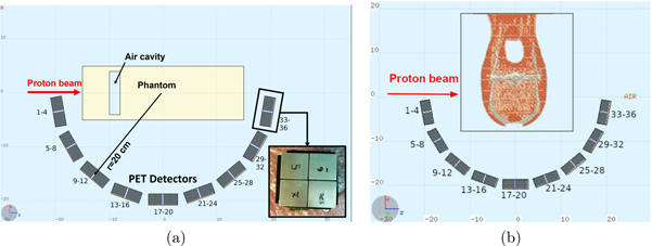
Figure 1. Schematics of the simulated setup obtained exploiting the FLUKA and FLAIR (Vlachoudis et al 2009) tools for CT import and visualization. The proton beam is impinging towards the positive Z direction in an homogeneous PMMA phantom in which an air cavity of variable thickness is in some cases present (a), and in an anthropomorphic phantom (b). In the latter, the beam traverses soft tissues, bone, and brain-like materials. The target is surrounded in both cases by an half-circle of 20 cm radius of PET modules, extended in the X–Z plane. In the inset in (a), the front (X–Y) view of a module is shown, featuring four S13900-3220LR-08 HPK PET detectors.
Download figure:
Standard image High-resolution imageA separated simulation set, featuring an anthropomorphic phantom as target, was also run to obtain some insight into the SER-PGT performance for a clinical-like scenario. The ALDERSON-RANDO 6 anthropomorphic phantom, made from tissue equivalent material modeled around a skeletal component (see figure 1(b)), was used for this preliminary evaluation. The phantom, routinely used in radiotherapy for dose measurements, was imaged by means of a CT scanner, then its DICOM file was imported with the FLUKA-FLAIR tools (Ferrari et al 2005, Vlachoudis et al 2009, Böhlen et al 2014) exploiting the Schneider parametrization for mapping the CT Hounsfield units into human tissues (Schneider et al 2000). For the detailed description of CT importing in FLUKA, see Battistoni et al (2016).
Being this a proof-of-concept, the emitted proton beam is monochromatic with null initial transverse size along the Z axis; afterwards, the particles are transported according to the physics model implemented in FLUKA (Battistoni et al 2015, 2016), which translates into lateral scattering and energy straggling. A total of nine different cases (beam energy and target cavity combinations) were simulated with the homogeneous phantom and are summarised in table 1. For the preliminary analysis with the anthropomorphic phantom, two different energies, corresponding to 110 MeV and 120 MeV, were simulated. The number of primary protons considered for each case of this study is 107. Each 107 protons run is repeated several times, so as to increase the statistical significance of the results and to set the free reconstruction and post-processing parameters. To adapt the method to the actual statistics of particles per spot in clinical treatments, the design of an eventual clinical system would be tuned to match the required statistics by increasing the active detector area or adding further detectors.
Table 1. Cases considered in the MC simulations with the homogeneous phantom. With 200 MeV beam energy, cavities of various sizes are present in the phantom, otherwise it is homogeneous. The third column contains the range in PMMA according to NIST PSTAR database (Berger et al 1998). Where air cavities are present, their stopping power has been neglected and the corresponding range is equal to the range in the homogeneous plus the cavity size.
| Proton beam energy (MeV) | Phantom | Range in target (cm) |
|---|---|---|
| 110 | Homogeneous | 8.0 |
| 140 | Homogeneous | 12.2 |
| 170 | Homogeneous | 17.0 |
| 200 | Homogeneous | 22.6 |
| 200 | 1 cm cavity | 23.6 |
| 200 | 2 cm cavity | 24.6 |
| 200 | 3 cm cavity | 25.6 |
| 210 | Homogeneous | 24.6 |
| 229 | Homogeneous | 28.4 |
PGT-based techniques rely on the precise time measurement of both the primary proton transit time and secondary photon arrival time. In the I3PET system the primary proton timing measurements will be performed by means of ultra-fast silicon detector strips (UFSDs). UFSDs are based on moderate-gain low-gain avalanche diodes (LGADs), with a thickness of few tens of μm and ensures a time resolution of tens of ps, with a signal duration of 2 ns (Giordanengo and Palmans 2018, Sola et al 2019, Vignati et al 2020). Consequently UFSDs can measure proton beams up to clinical rates with very limited signal pileup and excellent timing performance. Therefore, they have not been explicitly modelled in the simulation, since the bottleneck of TOF measurement relies in the secondary photon arrival time measurement.
This study also focuses on assessing the effectiveness of the algorithm proposed in section 2.1. Its performance will be primarily determined by the dimensions and ill-conditioning of the problem, as well as inconsistencies arising from possible data truncation and statistical fluctuations. Other physical phenomena will also contribute to deteriorate the accuracy of the results. To better identify the intrinsic limits of the algorithm, presently we neglect the contribution of false proton-photon coincidences at clinical beam rates. Those false coincidences strongly depend on the fine time structure of the beam, which is typically accelerator-dependent. The effect of false coincidences will be explored in a future work. Additionally, the concept presented here can be experimentally tested by operating the accelerator at a rate where the false coincidence rate is negligible, i.e. tens of MHz or less.
2.3. Data processing
We merge the information (i.e. timing and energy deposition) coming from every scintillating element belonging to the same PET detector; we consider as detector d each 8 × 8 channel block on which the system is based. Hence, we have 36 detectors of about 5 × 5 × 2 cm3 volume each, arranged in groups of four in each module (see figure 1 for reference). This choice is motivated by the PET detectors' dimension and features, which are optimised for the detection of 511 keV pairs: their usage to detect prompt photons implies some compromises. Many prompt photons in the MeV range suffer multiple Compton scattering inside the same detector. Moreover, despite the one-to-one coupling between scintillating elements and SiPM pixels in Hamamatsu S13900-3220LR-08 detectors, some preliminary experimental tests show that a significant amount of light is shared between adjacent pixels. These combined effects will eventually make impossible to identify the 3.2 mm element in which the photon has first interacted. The above-mentioned pixel output merging circumvents this potential issues and makes hence unnecessary to model the light sharing in the simulation.
The rules implemented in the data post-processing to model the above-mentioned effects are:
- to model the time resolution, individual secondary particle interactions in each 3.2 mm crystal elements are smeared with a 250 ps FWHM Gaussian;
- likewise, the single element energy resolution is set to 15%;
- a list of hits for each detector is then formed and sorted for each event;
- the element hits are finally merged into detector hits, the time assigned to each detector hit is the average of the pixel hits forming it, the energy corresponds to their sum.
The characteristics of the simulated PET detectors are based on state-of-the-art PET electronics coupled to SiPM and fast scintillators (Bugalho et al 2019), remaining on a conservative side to account for eventual performance degradation caused by the broader energy spectrum of photons with respect to the standard PET conditions.
The TOF acceptance window applied is 5 ns wide, while the energy window is between 1 and 6 MeV, no additional selection rule is applied. The former is set so as to be compliant with the energies of interest in proton therapy and with a reasonable detectors layout, the latter is set to accept the energy deposited by the photons of interest (Werner et al 2019). As also found in Marcatili et al (2020), the contribution of events depositing a low amount of energy, despite accepting some unwanted background, increases the statistics without significantly hampering the measurement accuracy.
2.4. System matrix calculation and MLEM implementation
First, the elements of the system matrix H and the sensitivity matrix S must be calculated, in order to enable the application of equation (5). To calculate the matrix elements, the quantities tTOF , z and tP must be discretized into bins. To investigate the influence of the bins width over the results, two different binning sets have been tested. The values used are summarised in table 2.
Table 2. Summary of the quantities, symbols and binning considered in the implementation of the system matrix H.
| Physical quantity | Quantity range | H index | Bin width | Number of bins | ||
|---|---|---|---|---|---|---|
| Setup1 | Setup2 | Setup1 | Setup2 | |||
| Detector number | 1–36 | d | 1 | 36 | ||
| tTOF | 0–5 ns | n | 100 ps | 50 ps | 50 | 100 |
| z | −20 cm to 20 cm | j | 0.5 cm | 0.25 cm | 80 | 160 |
| tP | 0–5 ns | p | 100 ps | 50 ps | 50 | 100 |
In our current implementation, H models the propagation of (unscattered) photons and the consequent detector response; its elements hdnj0 (i.e. for tP = 0) can be obtained by simulating photon sources along Z, which is the propagation direction of the pencil beam. In this case, tTOF is equal to tγ where tγ is the time required by the photon from its emission until its detection. To this end we used a dedicated Monte Carlo simulation, where 4.4 MeV photons are emitted with initial time equal to zero (i.e. tP = 0), from randomly-chosen evenly-distributed points along the beam axis Z, with random isotropic emission direction. The photons are then propagated in an empty medium (no target and no air). This model ignores the effects of photon interactions in the patient. (A more sophisticated model is considered below to investigate to what extend this simplification is justified.) If the prompt photons interact with any of the detectors (as in figure 1), their interaction time and energy deposition is scored and later post-processed in the same way as described in section 2.2. Further matrix elements for non-zero values of tP are obtained from hdnj0 exploiting the relationship

and shifting hdnj0 along the p index according to the chosen time bin width. It is important to point out that, in equation (7) the time associated to the target nuclei de-excitation and the subsequent emission of the photon was not included (Jacquet et al 2021). This MC-based technique to calculate the system matrix ensures accuracy in modelling the detector response to prompt photons, but it also requires sufficient statistics to avoid the propagation of uncertainties from the system matrix to the reconstructed emission distribution. To this end, 1.6 · 107 photons are simulated. Additionally, the symmetries present in the placement of the 36 detectors are exploited, thus enforcing a fourfold statistics increase.
To evaluate the eventual impact of attenuation and scattering of the photons inside the target, we have calculated a system matrix Hatt accounting also for those effects. To this end, we repeated the MC simulation described in this section including the homogeneous PMMA target, so as to straightforwardly obtain a system matrix whose effect in reconstruction can be compared to the original H.
The reconstruction algorithm is implemented in C++. Its running time is about 1 s for each iteration, with a single-thread implementation on a standard i3 notebook computer. No efforts have been made yet in profiling and optimising the code.
2.5. Post-processing of the reconstructed time-depth distribution
The results obtained by iterating equation (5) must be post-processed to extract meaningful information. The output of the iteration process described in equation (5) is a 2D histogram in the time-depth emission space (tP , z) which reflects the behaviour of the single protons behind each PG emission. On the other hand, we are interested in the collective behaviour of the proton beam determined by electronic interactions, i.e. on the average proton motion inside the target (see also Jacquet et al (2021)); therefore, the raw reconstructed time-depth distributions need to be post-processed, otherwise reconstruction artefacts and outliers would hamper the interpretation. First, a cut based on the initial beam velocity is applied in the (tP , z) emission space, then a threshold is applied to the resulting region of interest to extract the actual emission region of the prompt photons. Lastly, the surviving pixels are averaged along each p bin, so as to extract a z-versus-tP curve and ultimately the proton range.
The velocity-based cut exploits some quantities which are well-known and routinely measured in proton therapy, namely the beam initial energy, the emission point of the protons and its distance from the beginning of the target. It is consequently justified to restrict the (tP , z) emission space of the prompt photons to a ±20 cm wide spatiotemporal region around the initial proton beam speed. The outer borders of the (tP , z) space are excluded too. A preliminary study shows that the final result is quite insensitive to the exact amount of this selection, since the majority of the artefacts arise far from the beam motion region. This filter selects a region-of-interest (ROI) which is employed to extract the actual prompt photon emission and hence the range.
Once the ROI is set, the ROI pixels with a reconstructed emission lower than a given threshold are removed. The threshold t is calculated with respect to the pixel with the maximum reconstructed emission  , which is multiplied by a number T such as 0 < T < 1. Therefore, the rule for filtering the
  elements is

The surviving pixels indicate the region where most of the emissions occur. As the result of this step is quite sensitive to the actual T value, this free parameter is optimised in a subsequent step.
The last post-processing step is the so-called profiling, i.e. calculating the average z for each tP bin. This results in a z-versus-tP curve. We identify as particle range the maximum z value of the curve.
2.6. Early stopping and performance assessment
In MLEM reconstruction the convergence of the iterative equation (5) is guaranteed (Shepp and Vardi 1982, Lange et al 1984); however, the iterative process is stopped before the convergence, as MLEM might converge to a noisy image with non-physical features. Therefore, we must define the criteria to assess the optimal number of iterations. Moreover, the accuracy and precision in the reconstruction of the quantity of our interest in this study (i.e. the proton range) also depend on the post-processing threshold applied, as discussed in section 2.5. Given the low number of counts available in the data Y, it is also necessary to check the influence of the actual Y realization on the results. To that aim, we repeated the runs described in table 1 several times and divided them in two sets. The first set was used to find the best combination for the number of iterations and threshold to be applied, so as to maximise the accuracy and precision of range reconstruction with respect to the expected range (see also table 1). Then, the second set of repeated MC simulations was used to assess the actual reconstruction performance, thus avoiding the bias that would have been introduced by using the same dataset for both free parameters determination and performance assessment.
3. Results
3.1. System matrix calculation and model verification
The results of the MC simulation dedicated to the calculation of H can be visualised as a set of 2D time-depth histograms, i.e. tγ versus z (figure 2). Each histogram corresponds to a different d detector. The quantity scored in each histogram pixel is the number of detected events, which is proportional to the probability of a photon emitted in (tP = 0, z) to be detected after a time equal to tγ . Next, we exploit the translation symmetry of the system matrix, so that the actual H is directly calculated by summing tP to each distribution, i.e. by shifting them along the binning index p. The symmetries present in the detector arrangement are considered; in this case, since the beam is travelling along Z, there is a fourfold symmetry, originating a 4x increase in the statistics. In a more general case where the beam is emitted along a generic direction parallel to Z, however, the H calculation procedure must be repeated for each beam position.
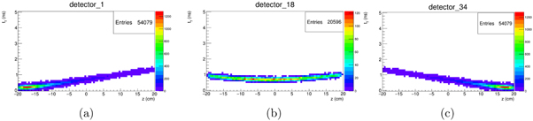
Figure 2. Visualisation of exemplary results of the Monte Carlo simulation dedicated to the system matrix calculation. The plots represents the number of photons emitted in Z (horizontal axis) detected after a time of flight equal to tγ (vertical axis). Plots (a) and (c) show the results for two detectors in the symmetrical leftmost and rightmost position with respect to the arrangement shown in figure 1, while (b) corresponds to a central one.
Download figure:
Standard image High-resolution imageTo verify the accuracy of the model behind H, we employ equation (1) and we do a dedicated scoring of the actual prompt photon emission in the MC simulation to compare HX* and Y*. The operation HX* is the so-called forward projection and X* and Y* are particular realizations of the random vectors X and Y, respectively. While Y* is directly obtained from the simulations, to create X*, the emission time and coordinates of prompt photons are scored during the simulation for every emission event, regardless of the event being detected or not by the scintillators. The binning of these data along the tP
and z directions leads to X*, as shown in figure 4(a). Its projection towards the detection space by means of equation (1), leads to a set of D vectors that can be now compared to Y* to assess the capability of our system matrix to describe the detection process. The results of this calculation are shown in figure 3 for four different detectors. A virtually perfect model with very high statistics would reproduce  as expected, this is not the case here because of the approximations introduced in the model (see 2.4) and limited statistics. Particularly, the current H fails in reproducing the tails of the measurements in the detectors placed in forward position. The main cause of this effect is that the system matrix only accounts for prompt photons isotropically emitted along the beam path, while a few of secondary neutrons and protons are mostly emitted forward. Hence, our model accurately reproduces the detection of the scintillators placed upstream and in general the rising edge of the tTOF
distributions, while the most significant differences are in the falling edges of the detectors placed downstream with respect to the beam direction. We observed that the discrepancies between the problem modelling described in sections 2.1 and 2.4 causes some inaccuracies in the spatiotemporal emission reconstruction and the presence of artefacts at the edges of the field of view; on the other hand, this proof-of-principle study focuses on range measurement, whose performance will be assessed in the following sections. More advanced models and dedicated compensation of background signals will be considered in the future.
as expected, this is not the case here because of the approximations introduced in the model (see 2.4) and limited statistics. Particularly, the current H fails in reproducing the tails of the measurements in the detectors placed in forward position. The main cause of this effect is that the system matrix only accounts for prompt photons isotropically emitted along the beam path, while a few of secondary neutrons and protons are mostly emitted forward. Hence, our model accurately reproduces the detection of the scintillators placed upstream and in general the rising edge of the tTOF
distributions, while the most significant differences are in the falling edges of the detectors placed downstream with respect to the beam direction. We observed that the discrepancies between the problem modelling described in sections 2.1 and 2.4 causes some inaccuracies in the spatiotemporal emission reconstruction and the presence of artefacts at the edges of the field of view; on the other hand, this proof-of-principle study focuses on range measurement, whose performance will be assessed in the following sections. More advanced models and dedicated compensation of background signals will be considered in the future.
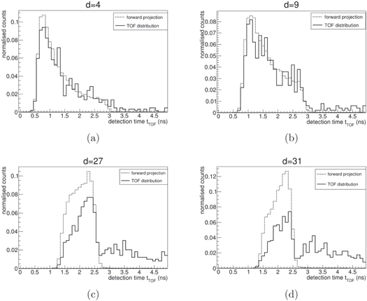
Figure 3. Comparison between tTOF distributions (continuous line) and forward projection of the simulated emission (dotted line) calculated by means of equation (1) for four detectors in different equally separated positions, from upstream (a) to downstream (d) (see figure 1 for the reference position). Each pair of plots is normalised to ease the comparison.
Download figure:
Standard image High-resolution image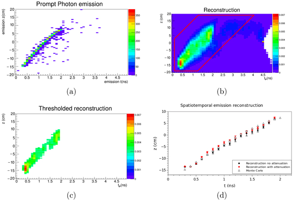
Figure 4. Exemplary post-processing and range evaluation. The Monte Carlo truth of the prompt photon emission scored in the simulation is shown in (a), while the result of the reconstruction after the MLEM iterations is shown in (b). The reconstructed spatiotemporal distribution is then cut in the (tP , z) space around the straight line given by the initial proton velocity (b, red polygon), to exclude the reconstruction artifacts such as the one in (b) at tP = 4.5 ns. Lastly, a threshold is applied (c), as described in section 3.2. Plot (d) displays the profiles of (a, triangles) and (c, black dots), averaged for seven independent simulation runs, the error bars correspond to the standard deviation across the runs (errors on Monte Carlo truth are negligible on this scale). Additionally, the same data were reconstructed with a system matrix Hatt accounting for the attenuation and scatter of the homogeneous phantom (see red dots). We define the reconstructed range as the point with the maximum z of the reconstructed profile shown in (d).
Download figure:
Standard image High-resolution image3.2. Reconstruction and post-processing
After the system matrix calculation and the (simulated) measurement process, it is then possible to apply the iterative equation (5) to reconstruct the emission distribution  of prompt photons in the (tP
,z) space. Figure 4(b) illustrates the method proposed here for a reconstruction using 10 iterations. It shape is similar to the actual emission shown in figure 4(a), but on the other hand its interpretation is hampered because of artefacts and noise; figure 4(c) shows the post-processing results as described in section 2.5, with a threshold calculated as in equation (8). Finally, the average of z along each temporal emission bin p of the post-processed reconstructed emission is shown in figure 4(d) (circles). For visual comparison purposes, we also report the results of the same profiling procedure applied on the actual prompt photon emission, as shown in figure 4(d) (triangles).
of prompt photons in the (tP
,z) space. Figure 4(b) illustrates the method proposed here for a reconstruction using 10 iterations. It shape is similar to the actual emission shown in figure 4(a), but on the other hand its interpretation is hampered because of artefacts and noise; figure 4(c) shows the post-processing results as described in section 2.5, with a threshold calculated as in equation (8). Finally, the average of z along each temporal emission bin p of the post-processed reconstructed emission is shown in figure 4(d) (circles). For visual comparison purposes, we also report the results of the same profiling procedure applied on the actual prompt photon emission, as shown in figure 4(d) (triangles).
In figure 4(d) we also assessed the impact of the system matrix Hatt on the reconstructed distribution. Neither the reconstructed profile accuracy nor the range assessment are significantly improved when considering photon attenuation and scattering effects. In a real application, a model of these effects would be calculated based on the available CT, which might differ from the true values of the attenuation coefficients. In fact, changes in the patient morphology are a source of range deviations. At this stage, it is not clear if there might be benefits in the use of Hatt instead of the non-biased H.
It must be highlighted that up to this point two parameters have been set on the basis of visual evaluation, but they have not yet been optimised in order to provide the best performance in terms of range measurement. Namely, these parameters are the number of iterations kmax for stopping the iterations of equation (5) and the threshold T applied in the post-processing of the  distribution, as defined in equation (8). The necessary optimisation study will be addressed in the following section.
3.3. Parameters optimisation for range reconstruction
The number of iterations kmax and the post-processing threshold T must be jointly optimised, as the features of the resulting thresholded distribution depend on both of them in an interdependent manner. As usual in MLEM-related solutions, increasing the number of iterations amplifies the noise of the reconstructed image, while stopping the iterations too early results in a low-resolution blurred image. At the end of the reconstruction, the threshold T applied to extract the actual spatiotemporal  emission cluster according to equation (8) has a major effect on its extension and hence on the reconstructed range. Moreover, the reconstructed distribution might exhibit different features according to the binning of choice, i.e. setup 1 and 2 as defined in table 2.
The available datasets have been divided into two independent groups, one dedicated to the optimisation of kmax and T, the other to assess the range reconstruction performance. The optimisation datasets are 63 in total, i.e. 7 repetitions of 107 protons irradiation for each of the cases reported in table 1. We varied kmax between 1 and 100 in steps of 1 and T from 0 to 0.9 in steps of 0.0025. For each combination of those parameters the difference between the reconstructed range and the expected one (table 1, third column) is calculated. Then, it is possible to assess which combination provides the best results in terms of accuracy and precision, by calculating the average and the standard deviation of the above-mentioned differences respectively, and finding their minimum. The procedure is repeated for each of the two binning setups defined in table 2.
The results of the optimisation procedure indicate that the overall best results are provided by binning setup 2, which is related to a finer binning, as shown in figure 5. The green areas depicted in plots (a) and (c) show that average range errors below 1 cm are possible for both setups. Whereas this area extends over a large range of iterations for setup 1, it is larger for setup 2, i.e. a larger number of parameter combinations allows for accurate results. The standard deviation related to the areas with the smallest errors is lower for setup 2 than for setup 1.
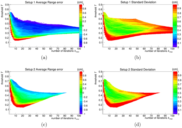
Figure 5. Average difference (m) and absolute standard deviation (m) in reconstruction range assessment, as a function of the number of iterations kmax and post-processing threshold T, relative to the optimisation datasets as described in section 3.3. The first row (a), (b) represents the results for the binning setup 1, while the second (c), (d) those of setup 2. The white areas are relative to the results below the range indicated in the lookup table, or when T is too high so that not every case considered could provide at least one surviving point for range evaluation.
Download figure:
Standard image High-resolution imageAlthough the general trend of the distributions is the same, it is also observable with a pixel-wise analysis that the mean error and its standard deviation do not follow exactly the same pattern. Setting a rule to find the absolute best compromise between those two quantities is beyond the scope of this work and moreover this might lead us to the trap of over-optimisation. Hence we identified for setup 2 the pair  and T = 0.56 to provide a satisfying performance, i.e. 0.2 cm average error and 0.4 cm standard deviation. This particular parameter combination was chosen by considering first a region in the distribution where both the average range error and standard deviation have a stable trend, without jumps in the values or white pixels nearby (which correspond to values outside the lookup table or where the reconstruction failed); then, inside this region, the (kmax, T) pair with the lowest number of iterations was chosen to reduce computing time, in the view of possible on-line applications.
3.4. Range reconstruction performance
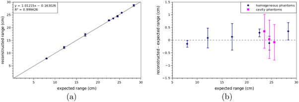
The reconstructed range when compared to the ground truth exhibits a perfectly linear correlation with a slope equal to 1.01 and a systematic under-estimation of 0.16 cm, as shown in figure 6(a). The binning and the parameters kmax and T are those found with the optimisation described in section 3.3. The 63 datasets used to study the performance are independent from those used to calibrate the reconstruction parameters, so it is reasonable to repeat the calculation of the average error and its standard deviation. On average the difference is 0.1 cm (up to 0.3 cm) and 0.5 cm standard deviation (up to 0.8 cm, figure 6(b)), which are comparable with the optimisation datasets.
Figure 6. (a) Reconstructed range versus expected range for each simulated case (table 1). The range is reconstructed as described in section 3.2 with the parameters described in section 3.3. Each point corresponds to the average reconstructed range of each of the nine different cases, error bars correspond to the standard deviation of the seven runs executed for each case. A straight line resulting from the linear regression is also shown, together with its equation. (b) Difference between reconstructed and expected range, for homogeneous targets (blue) and targets with cavity (pink). Reconstruction parameters and error bars are calculated as in (a).
Download figure:
Standard image High-resolution image
3.5. Preliminary results with the anthropomorphic phantom
The range inside the anthropomorphic phantom was evaluated considering the binning and the reconstruction parameters optimized in section 3.3. Both simulations (110 and 120 MeV) were repeated 10 times with independent runs to increase the statistical significance. The calculated mean range and corresponding standard deviation amount to (11.4 ± 0.6) cm and (12.1 ± 0.3) cm, for 110 and 120 MeV, respectively. The difference between the two reconstructed ranges was compared to the difference of the expected ranges, to preliminary assess the method feasibility with not-homogeneous tissues. The expected range was calculated as the 80% of the distal fall-off of the dose scored in the simulation (Paganetti 2012a). The difference between the expected ranges of the two energies was of 1.4 cm, while the difference of the reconstructed range of the two energies was equal to (0.7 ± 0.7) cm.
Even though only preliminary, this result is somehow encouraging towards the SER-PGT application in more clinical-like scenarios.
4. Discussion
4.1. SER-PGT for range monitoring
In this study we have presented multi-detector prompt gamma timing, a new approach to the exploitation of prompt photons measurements, allowing the reconstruction of the proton range inside the target. Monte Carlo simulations show that the reconstructed range is in agreement with the expected value within few millimetres (detailed in figure 6(b)), for beam energies ranging from 110 to 229 MeV, impinging on an homogeneous PMMA target with or without air cavities inside, considering 107 primary protons. Moreover, a preliminary analysis simulating an anthropomorphic phantom shown the capability of reconstructing two different energies with an accuracy within 0.7 cm, proving the capability of the implemented reconstruction to assess clinical-like conditions.
This study was focused on the implementation and optimisation of SER-PGT with PET detectors, to assess the feasibility of a scanner capable of performing both prompt photons and in-beam PET measurements, providing richer information without increasing the scanner cost or its size. Hence, the presented results are significant for this kind of experimental setup. Note that the setup shown in figure 1 is not suitable for PET imaging as it is. Since this work focuses on prompt photons signal, only half a ring was considered. Implementing SER-PGT for a complete PET system would be straight forward. For the considered scenario, where the beam is at the isocenter (ie. x = 0, y = 0), the second half-ring would contribute to improve the statistics but would not add any additional information because of the symmetry of the design. For off-center beams, a specific system matrix must be computed for each beam position, and a second half-ring might bring additional information due to the non-symmetry of the problem. SER-PGT may be also implemented with detectors optimised for timing measurements in the MeV range, likely providing a better performance in prompt photons monitoring at a lower cost with respect to the bi-modal solution, since it could be based on a lower number of channels, dramatically decreasing the electronics complexity.
A key role in PGT is played by the technique used to measure the timing of the primary protons and by their rate. In this study, we decided to (coarsely) model the behaviour of ultrafast silicon detectors (UFSD). Such detectors are candidates to provide the basis of next-generation beam monitors in particle therapy. They are able to measure particle timing with a resolution of about 30 ps up to clinical rate thanks to the short (2 ns) signal duration and fine segmentation. Hence, the bottleneck in TOF resolution for this configuration is the PET detector, whose timing resolution was set to 250 ps FWHM. It is also well known by other studies (Golnik et al 2014, Hueso-González et al 2015, Marcatili et al 2020) that the proton bunch duration in cyclotrons for PT is as short as few ns, therefore it is possible to use a single-channel fast detector or even the accelerator radiofrequency to measure the bunch time and exploit it for the start of the TOF measurement, at the price of a degraded resolution. The model presented in this study can be adapted to this case too, modifying the system matrix calculation and incorporating the actual time resolution. In this study we neglected the random coincidences arising in TOF measurement at clinical-like primary particle rates. This approximation can be accounted for by modifying the forward projection term in equation (5) (Oliver and Rafecas 2016). However, this can be done only after a thorough characterisation of the fine time structure of the beam, which depends on the specific facility where the measurement is performed. Future experimental work will explore the beam structure by means of UFSDs and will possibly implement any of the well known random corrections techniques in equation (5).
An extremely important feature specific of the SER-PGT formulation presented in this study is the absence of any kind of assumption on target composition, density or stopping power. This drastically strengthens the robustness of the method, as it allows to directly estimate the beam range without a calibration curve. Moreover, the role of the Monte Carlo simulation is limited to the system matrix calculation (i.e. the propagation in the void and detection of photons uniformly emitted along the Z axis). In other words, the SER-PGT method does not rely on the nuclear interaction, excitation and de-excitation models implemented in the Monte Carlo framework of choice and on their validation, therefore the system matrix could be also obtained by an analytical model that takes into account the geometry of the problem, i.e. the detectors position and efficiency. On the other hand, an additional system matrix, accounting for both scatter and attenuation effects, was considered for the reconstruction. However, result show marginal improvement over the non-biased system matrix. To include scatter and attenuation in the system model, anatomical information about the patient is required. At the same time, the need of range verification also arises from possible mismatches between the CT and the true patient anatomy during the treatment, which is a conundrum in itself. In any case, for the energy range and target here considered, attenuation might be negligible, or still less significant with respect to PET signals.
The MLEM-based method we presented is well suited to solve the inverse problem we described in section 2.1, as we implemented a linear description of the problem, and the measurements follow a Poisson distribution. Nevertheless, the system matrix H ignores the contribution of certain phenomena. Particularly, the model only considers the emission of prompt photons arising from nuclear de-excitation along the beam path, not taking into account that some photons can originate from positions other than the beam axis. Also the eventual detection of other secondary particles is ignored. However, it is to highlight the robustness of the method with respect to the weak points of PET detectors, namely particle identification and energy-based discrimination in the MeV range. In any case, the contribution of other secondary particles could be compensated, at least partially, either at the data level (filtering), or during the reconstruction, by modelling their contribution within the system matrix or using estimates of the background signals in the forward projection step.
For this proof-of-principle study, the system model assumes that the proton path can be described by a perfect line. The knowledge of the finite transverse size of the beam, which is monitored in real-time in clinics by means of dedicated detectors in the beamline nozzle, can be included in the model. In principle, this might also require to extend the spatial dimension of the spatial domain, i.e. to reconstruct (x, y, z) − tP instead of z − tP . Even though this extension is rather straight-forward to implement, it increases the number of unknowns for the same amount of information. This approach is computationally more demanding, and will be addressed in future works.
Another approximation made in the system matrix model is neglecting emission lines other than 4.4 MeV. Moreover, the nuclear de-excitation time is also neglected, which can be somehow significant for some reactions. Namely, the gamma emission after 16O(p,p')16O* has a mean lifetime of 27 ps, while that of 40Ca(p,p')40Ca* is of 47 ps. The former reaction is more significant at the end of the proton range, while the latter in the bones (Jacquet et al 2021). Further improvements might be needed to study the impact of multiple emission lines and de-excitation times impact on the SER-PGT method performance.
The results of the reconstruction and post-processing are remarkably robust with respect to the number of MLEM iterations and post-processing threshold. As shown in figure 5, the standard deviation of the range measurement is about 0.5 cm for both the tested binning configurations, considering 107 primary protons. An additional aspect that strengthens the method robustness is to be found in the preliminary analysis of the anthropomorphic phantom: no attempts were made to specifically optimize the reconstruction; on the contrary, the parameters found for the homogeneous phantom reconstruction were used, yielding very good results. Future studies should include the full performance assessment in not-homogeneous materials, including bones and any other biologically significant material.
4.2. SER-PGT outlook and potential applications
The most interesting innovation in the method proposed in this study is the fact that equation (5) provides an output in the emission time-depth domain, (tP , z), consisting in samples of the z-versus-tP curve describing the proton motion inside the target (see also Jacquet et al (2021)). The results presented in this paper, however, cannot be directly applied to study the proton motion, since the free parameters of the method (namely: number of iterations and post-processing threshold) are optimised for the reconstruction of the range, which is identified as the maximum z value of the z-versus-tP curve. Moreover, as shown in figure 3 and discussed in section 4.1, the artefacts that affect the results would hamper the accuracy of the reconstructed proton motion. Nonetheless, SER-PGT has a strong potential to be furthermore explored, and we aim to optimise for direct proton-motion reconstruction. This paves an exciting and never-before-explored way towards the direct in-vivo assessment of the kinematics of the particles along their path, which is a quantity strongly related to the target stopping power.
Lastly, future studies will include the pursuit of a more effective compromise between the PET and SER-PGT modalities (detectors, electronics and layout), so as to also optimise the proton motion reconstruction, which is in the authors' opinion the most interesting prospect given by the results of the proposed method.
5. Conclusion
In this study we have introduced SER-PGT, an approach able to estimate the time-depth distribution of the prompt photon emission. In the current implementation, the method relies on the MLEM algorithm followed by dedicated postprocessing steps. The method was tested by means of accurate Monte Carlo simulations; it has provided accurate results for range measurement and shows very promising properties which support further investigations.
SER-PGT has the significant feature of not requiring any prior information about the target (i.e. the patient's) composition. This is encouraging towards the ultimate in-vivo application of the method. The method has been tested in this study by means of in-beam PET detectors, with a range resolution of about 0.5 cm between 110 and 229 MeV with 107 protons. The study of a dedicated system optimised for prompt photons detection will allow the possible optimisation of the direct reconstruction of the particle motion and their kinematics inside the patient body.
Acknowledgments
This work is supported by the INFN Group 5 Young Investigators Grant I3PET, and partly by the German Research Foundation (DFG) with Project Number 383 681 334.
The CT of the ALDERSON-RANDO Phantom has been provided by CNAO (Pavia, Italy). The authors would like to thank Mario Ciocca and all the CNAO staff involved.
Additional information
The authors declare no competing interests.