
Abstract
To investigate the impact of training sample size on the performance of deep learning-based organ auto-segmentation for head-and-neck cancer patients, a total of 1160 patients with head-and-neck cancer who received radiotherapy were enrolled in this study. Patient planning CT images and regions of interest (ROIs) delineation, including the brainstem, spinal cord, eyes, lenses, optic nerves, temporal lobes, parotids, larynx and body, were collected. An evaluation dataset with 200 patients were randomly selected and combined with Dice similarity index to evaluate the model performances. Eleven training datasets with different sample sizes were randomly selected from the remaining 960 patients to form auto-segmentation models. All models used the same data augmentation methods, network structures and training hyperparameters. A performance estimation model of the training sample size based on the inverse power law function was established. Different performance change patterns were found for different organs. Six organs had the best performance with 800 training samples and others achieved their best performance with 600 training samples or 400 samples. The benefit of increasing the size of the training dataset gradually decreased. Compared to the best performance, optic nerves and lenses reached 95% of their best effect at 200, and the other organs reached 95% of their best effect at 40. For the fitting effect of the inverse power law function, the fitted root mean square errors of all ROIs were less than 0.03 (left eye: 0.024, others: <0.01), and the R square of all ROIs except for the body was greater than 0.5. The sample size has a significant impact on the performance of deep learning-based auto-segmentation. The relationship between sample size and performance depends on the inherent characteristics of the organ. In some cases, relatively small samples can achieve satisfactory performance.
Export citation and abstract BibTeX RIS

Original content from this work may be used under the terms of the Creative Commons Attribution 4.0 licence. Any further distribution of this work must maintain attribution to the author(s) and the title of the work, journal citation and DOI.
1. Introduction
Segmentation of the target volumes (TVs) and regions of interest (ROIs) are essential steps in radiotherapy (Citrin 2017). Compared to 2D- or 3D-conformal radiotherapy, intensity-modulated radiotherapy (IMRT) can deliver a more conformal dose distribution to the TVs and notably spare ROIs with fewer radiation-related toxicities in head and neck cancer (HNC) (Kosmin et al 2019). The gradients of the dose distribution are steep outside the planning target volume, and the structures can receive fewer absorbed radiation doses if they are particularly delineated as ROIs in IMRT (2010). It is obviously important to delineate the ROIs accurately, and tumor control and radiation toxicity have shown a high correlation with the accuracy of TV and ROI delineation (Mukesh et al 2012, Walker et al 2014).
However, manual delineation that is performed by a physician on computed tomography (CT) and/or magnetic resonance (MR) images is challenging, time-consuming, and subjective, with potentially large inter- and intraobserver variability (Brouwer et al 2015). This variation in ROIs delineated by different physicians has been shown to be not only theoretical but also has significant dosimetric effects on patients (Voet et al 2011). Moreover, adaptive radiotherapy requires that the treatment be adapted anatomically or biologically to the changes of patients or tumors during the course of treatment (Witt et al 2020). This requires rapid recontouring of the TVs and ROIs to re-evaluate the dosimetry and consider whether to replan during a fraction of radiotherapy in real-time.
The time required for delineating ROIs and TVs is an obstacle to adaptive radiotherapy, which hinders the development of radiotherapy to some extent. Rapid auto-segmentation can alleviate these problems and promote the development of adaptive radiotherapy (Kosmin et al 2019).
Head-and-neck ROI segmentation is a typical application scenario of auto-segmentation. The efficacy and safety of head-and-neck radiotherapy requires accurate ROI segmentation. More recently, deep learning-based auto-segmentation techniques have been shown to provide significant improvements over many traditional approaches (Cardenas et al 2019). Many studies have investigated using deep learning techniques to segment these organs (Ibragimov and Xing 2017, Ren et al 2018, Tong et al 2018, Hänsch et al 2019, Liang et al 2019, Men et al 2019, van Rooij et al 2019, Zhu et al 2019, Liu et al 2020), and most have focused on improving the algorithms (Lundervold and Lundervold 2019).
Deep learning-based auto-segmentation relies on the availability of annotated datasets. It follows the general principle of deep learning: the more data there are, the better the results (Cho et al 2015). However, for medical images, high-quality annotated datasets are scarce and require specialized medical knowledge, standardized protocols and considerable time and effort. The development of transfer learning (Torrey and Shavlik 2009) and data augmentation (Goodfellow et al 2016) may reduce the data size requirement. However, annotation is still one of the key issues in medical image auto-segmentation. In some cases, it may take more time and effort than the algorithm development itself (Tajbakhsh et al 2020).
Therefore, it is important to estimate the required training sample size before deep learning-based auto-segmentation application development. If the required sample size can be estimated by setting performance goals and preliminary experiments, it may help researchers and developers design better research and software. Moreover, the impact of the ROI characteristics on the relationship between model performance and sample size needs to be further explored.
Three stuies (Hänsch et al 2019, Zhu et al 2019, Narayana et al 2020) have investigated the training sample size of medical image auto-segmentation. Two studies showed that by increasing the size of the training dataset, the performance of auto-segmentation may be improved (Hänsch et al 2019, Zhu et al 2019). However, these two studies were mainly focused on algorithm development, and no further analysis was performed. Narayana systematically investigated the impact of training size on 4 brain tissue segmentations on MRIs and indicated that the Dice similarity coefficient (DSC) of all tissues increased at the beginning and then stagnated (Narayana et al 2020).
Compared to brain tissue auto-segmentation, head-neck ROIs auto-segmentation is a common task in radiotherapy. It involves more than 10 organs with different structural characteristics, such as the spinal cord, which is a long organ extending across many slices, and the eyes, which only appear on a few slices with a small volume. This task may be more suitable for training sample size investigations.
In this study, a large head-and-neck dataset with 14 annotated ROIs was used to investigate the effect of the training sample size. Auto segmentation models are established with different training sample sizes and evaluated on an independent test dataset. Furthermore, we try to establish a prediction model that can be used to estimate model performance or the training sample requirement with some preliminary experiments.
2. Materials and methods
2.1. Images and segmentation
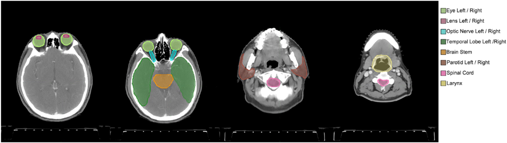
From February 2009 to April 2016, a total of 1160 patients with HNC who received radiotherapy at the Fudan University Shanghai Cancer Center were consecutively enrolled in this study. The treatment planning CT images and ROI delineation were collected in DICOM format. None of the CT images were contrast-enhanced. All patients' scans were obtained with the same CT scanner using the same imaging protocol (350 mA tube current, 120 kVp tube voltage, 0.92 × 0.92 mm pixel size, 5 mm thickness, 512 × 512 matrix). No additional CT preprocessing was performed before physician delineating. Fourteen ROIs were segmented by dozens of physicians in clinical practice with same consensus guidelines (Brouwer et al 2015), including the brainstem, spinal cord, eyes, lenses, optic nerves, temporal lobes, parotids, larynx and body. Paired ROIs were divided into left and right (figure 1). All images and their delineations were imported into MIM (MIM Software Inc., Cleveland, OH) to be manually checked by a physicist to avoid significant data errors, such as incorrect ROI naming.

Figure 1. Manually segmented ROIs of a randomly selected patient from the dataset. Four CT scan slices were selected to present the 14 ROIs clearly.
Download figure:
Standard image High-resolution image2.2. Deep learning algorithm for segmentation
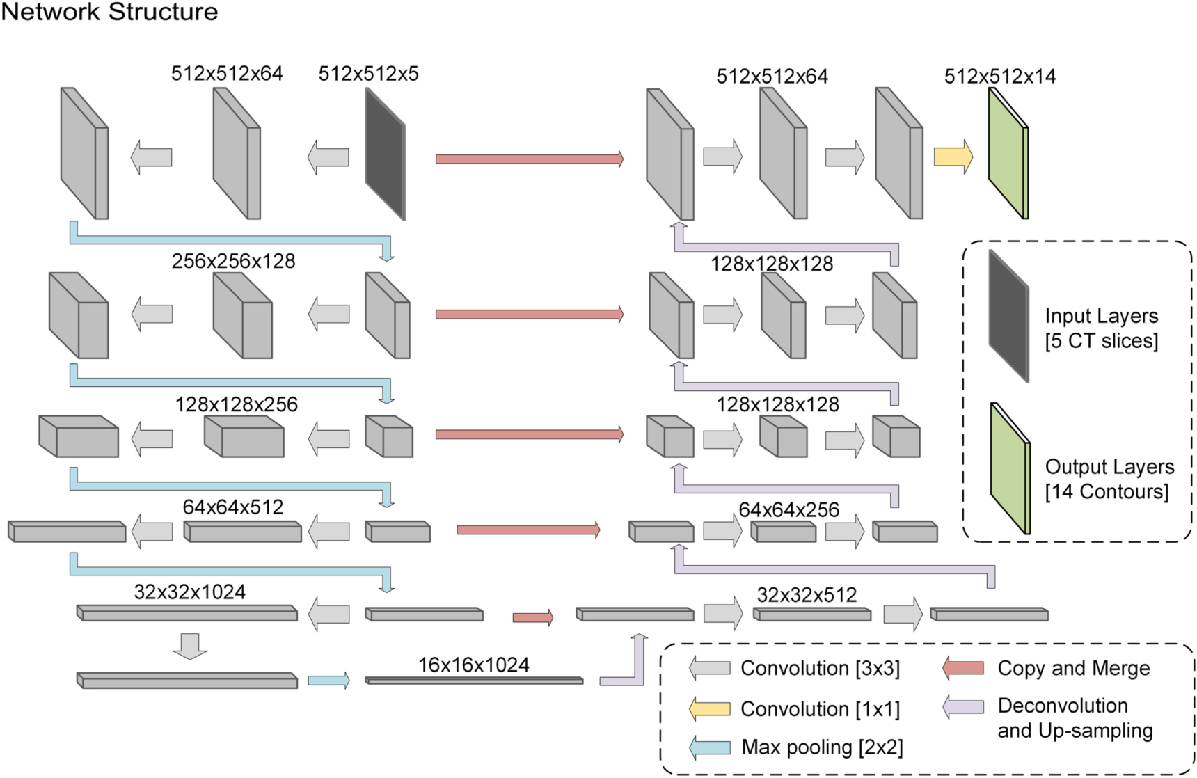
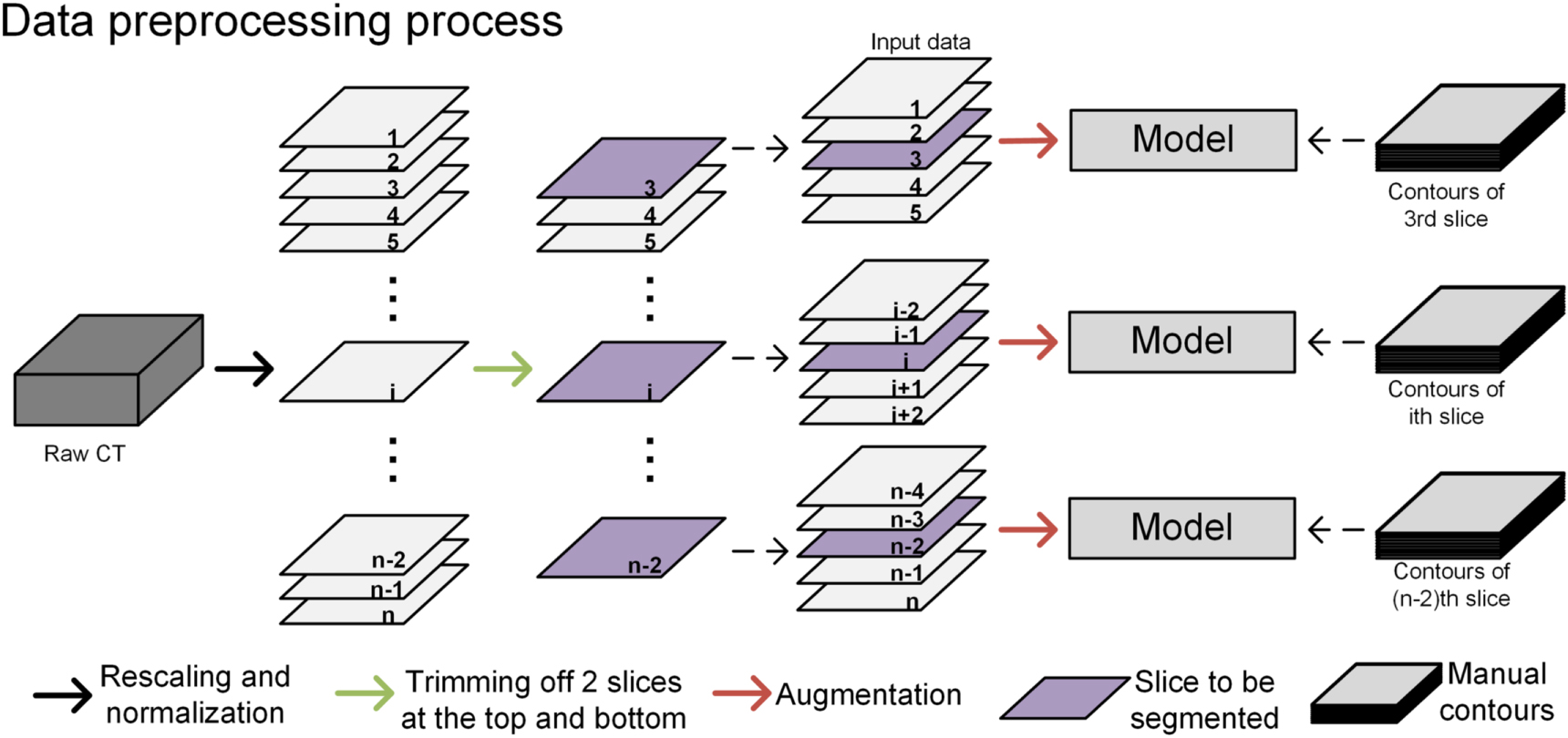
The model we used in this study was the U-net (Ronneberger et al 2015), which has been the 'baseline net' for organ and tumor segmentation in recent studies (Vrtovec et al 2020). The U-net's structure is shown in figure 2. The details of the U-net are provided in our previous manuscript (Wang et al 2018). The input was 5 CT slices and the output was 14 ROIs in 14 channels. Figure 3 shows the process of importing data into the model. First, the original CT is preprocessed, including scaling resolution and density normalization, and then all the images between the third layer and the third layer from the end are used to train the model layer by layer. When segmenting a CT slice, we input a 5 CT slices centered on it, which enables the model to make use of part of the spatial information about this CT slice. The 5 CT slices and the manual delineation corresponding to its middle slice are used together to train the model to segment on the middle CT slice.

Figure 2. Architecture of the U-net used for HNC auto-segmentation. The image dimension is denoted at the top.
Download figure:
Standard image High-resolution image
Figure 3. The process of data preprocessing. The rescaling resolution was 512 × 512 and the image density will be normalized to between 0 and 1.
Download figure:
Standard image High-resolution imageAll models in all training processes use the same hyperparameters. For iteration, all models had trained 50 epochs and performed 12 500 iterations in each epoch. The summation of all ROIs' 1—Dice index was employed as the loss function. The learning rate was 1e−4, and RMSprop was used as the optimizer. All models were converged with these settings. The model was implemented in Keras (Chollet 2015), and all calculations were performed with a GeForce GTX1080Ti GPU.
2.3. Dataset, data augmentation and model training
The total workflow is presented in figure 4. First, an independent test dataset was created with 200 patients randomly selected from the whole dataset for performance evaluation. Then, eleven different training datasets, which included 10, 20, 30, 40, 80, 120, 160, 200, 400, 600, and 800 patients, were generated by randomly selecting them from the remaining 960 patients with different random seeds.

Figure 4. Overview of the workflow.
Download figure:
Standard image High-resolution imageData augmentation (Goodfellow et al 2016) is a common strategy used to alleviate the training size requirements. We implemented two argumentation processes in this study, including gray level disturbance and shape disturbance. The CT images' gray values multiplied a number that was randomly selected from 0.9 to 1.1 and added another random number from −0.1 to 0.1 to the gray level disturbance. Then, the CT images and binary contour images were deformed using affine transform. The deformation algorithm used in this study was divided into two steps. First, we obtained the coordinates of the three vertexes (top left, top right, and bottom left), and then each point was shifted randomly in the range of [−1, 1] * image length (512 in our study). All CT images and binary contours were affine transformed by these transformations. Data augmentation was only used in the process of network training.
Each training dataset was used to train a deep learning-based segment model with the same network structures and hyperparameters (such as epochs and iterations). Eleven auto-segmentation models (m10, m20, m30, m40, m80, m120, m160, m200, m400, m600, and m800) were developed corresponding to these training datasets. For example, m10 and m800 are established by this method; that is, a patient is randomly selected from a training set of 10 and 800 samples, respectively, and after data augmentation, it is input into U-net for training, and all processes are repeated 12 500 times as an epoch. All models were trained with a total of 50 epochs. Then, the test dataset was applied to all of the models. For robustness against varying conditions, the whole process, including test dataset sampling, was performed four times.
2.4. Performance evaluation
The performance was evaluated by computing the DSC as below:

where A is the volume of the ground-truth segmentations (manually delineated by the physician); B is the volume of the auto-segmentation contours; and A ∩ B is the volume that the manual segmentation and auto-segmentation contours have in common. The calculation of volume was based on pixels in our study. The DSC can range between 0 and 1 (0 = no overlap, 1 = complete overlap). A higher DSC value indicates that the corresponding model works better.
Meanwhile, to demonstrate the increasing trend, a normalized DSC was calculated by dividing each ROI's best performance.
2.5. Performance estimation model
An inverse power law function was used to establish the relationship between the mean DSC and the training sample (equation (2)) (Mukherjee et al 2003, Figueroa et al 2012, Narayana et al 2020):

This model was fitted by the nonlinear weighted least squares method as described by Figueroa et al (Mukherjee et al 2003).
To investigate the accuracy of the performance estimation model, we used the performance results from fewer than 200 training samples (m10 ∼ m200) to create the model and compared them to the model with full performance results (m10 ∼ m800). The prediction power was evaluated by R square and root mean square error (RMSE). The estimation model fitting and evaluation were performed in R (version 3.0).
3. Results
3.1. Performance evaluation
Table 1 shows the DSCs of the 11 deep learning models for the 14 ROIs. The DSCs increased with the increase in training sample size for all ROIs for the entire trend. Meanwhile, the change pattern varied between different ROIs. The m800 model showed the best performance for six ROIs, including the body (DSC: 0.988), left eye (0.863), optic nerves (left: 0.630, right: 0.638) and temporal lobes (left: 0.765, right: 0.774). Other ROIs achieved the best performance in the m600 for the brainstem (0.825), larynx (0.746), spinal cord (0.804) and lenses (left: 0.676, right: 0.658) and m400 models for the right eye (0.862) and parotids (left: 0.783, right: 0.787).
Table 1. The DSC values for the ROIs segmented with different training sample sizes.
| Dice similarity coefficient (mean ± std) | |||||||
|---|---|---|---|---|---|---|---|
| Training size | Brain stem | Eye L | Eye R | Lens L | Lens R | Optic nerve L | Optic nerve R |
| 10 | 0.780 ± 0.067 | 0.760 ± 0.145 | 0.808 ± 0.095 | 0.536 ± 0.173 | 0.553 ± 0.163 | 0.553 ± 0.147 | 0.572 ± 0.140 |
| 20 | 0.804 ± 0.059 | 0.846 ± 0.050 | 0.845 ± 0.047 | 0.595 ± 0.148 | 0.591 ± 0.151 | 0.584 ± 0.144 | 0.599 ± 0.139 |
| 30 | 0.800 ± 0.057 | 0.834 ± 0.078 | 0.835 ± 0.065 | 0.596 ± 0.149 | 0.593 ± 0.153 | 0.566 ± 0.147 | 0.581 ± 0.147 |
| 40 | 0.806 ± 0.057 | 0.844 ± 0.076 | 0.842 ± 0.081 | 0.603 ± 0.143 | 0.597 ± 0.148 | 0.586 ± 0.142 | 0.595 ± 0.139 |
| 80 | 0.808 ± 0.056 | 0.849 ± 0.075 | 0.850 ± 0.081 | 0.630 ± 0.153 | 0.625 ± 0.153 | 0.598 ± 0.147 | 0.606 ± 0.143 |
| 120 | 0.811 ± 0.055 | 0.851 ± 0.077 | 0.850 ± 0.081 | 0.623 ± 0.155 | 0.627 ± 0.155 | 0.598 ± 0.145 | 0.604 ± 0.145 |
| 160 | 0.814 ± 0.057 | 0.852 ± 0.076 | 0.851 ± 0.082 | 0.634 ± 0.146 | 0.626 ± 0.156 | 0.590 ± 0.149 | 0.604 ± 0.140 |
| 200 | 0.816 ± 0.057 | 0.854 ± 0.077 | 0.850 ± 0.086 | 0.646 ± 0.147 | 0.634 ± 0.153 | 0.601 ± 0.152 | 0.607 ± 0.148 |
| 400 | 0.822 ± 0.055 | 0.861 ± 0.077 | 0.862 ± 0.082 a | 0.651 ± 0.140 | 0.653 ± 0.147 | 0.607 ± 0.140 | 0.621 ± 0.139 |
| 600 | 0.825 ± 0.058 a | 0.859 ± 0.076 | 0.861 ± 0.083 | 0.676 ± 0.139 a | 0.658 ± 0.149 a | 0.614 ± 0.149 | 0.627 ± 0.145 |
| 800 | 0.820 ± 0.062 | 0.863 ± 0.076 a | 0.860 ± 0.082 | 0.664 ± 0.138 | 0.653 ± 0.144 | 0.630 ± 0.145 a | 0.638 ± 0.140 a |
| Training Size | Temporal lobe L | Temporal lobe R | Parotid L | Parotid R | Spinal cord | Larynx | Body |
| 10 | 0.741 ± 0.131 | 0.743 ± 0.127 | 0.752 ± 0.079 | 0.747 ± 0.079 | 0.767 ± 0.085 | 0.722 ± 0.118 | 0.987 ± 0.010 |
| 20 | 0.727 ± 0.100 | 0.739 ± 0.105 | 0.769 ± 0.078 | 0.765 ± 0.077 | 0.789 ± 0.079 | 0.724 ± 0.119 | 0.987 ± 0.009 |
| 30 | 0.736 ± 0.114 | 0.756 ± 0.109 | 0.772 ± 0.079 | 0.771 ± 0.077 | 0.782 ± 0.080 | 0.738 ± 0.111 | 0.986 ± 0.009 |
| 40 | 0.745 ± 0.103 | 0.755 ± 0.104 | 0.769 ± 0.087 | 0.768 ± 0.090 | 0.789 ± 0.078 | 0.725 ± 0.120 | 0.988 ± 0.007 |
| 80 | 0.750 ± 0.110 | 0.765 ± 0.111 | 0.773 ± 0.089 | 0.772 ± 0.091 | 0.785 ± 0.079 | 0.729 ± 0.112 | 0.988 ± 0.008 |
| 120 | 0.746 ± 0.107 | 0.753 ± 0.103 | 0.769 ± 0.092 | 0.775 ± 0.092 | 0.793 ± 0.084 | 0.743 ± 0.119 | 0.988 ± 0.007 |
| 160 | 0.758 ± 0.112 | 0.770 ± 0.110 | 0.779 ± 0.089 | 0.779 ± 0.090 | 0.781 ± 0.091 | 0.746 ± 0.114 | 0.988 ± 0.007 |
| 200 | 0.756 ± 0.113 | 0.767 ± 0.110 | 0.780 ± 0.092 | 0.778 ± 0.094 | 0.795 ± 0.087 | 0.739 ± 0.125 | 0.987 ± 0.009 |
| 400 | 0.753 ± 0.110 | 0.768 ± 0.109 | 0.783 ± 0.090 a | 0.787 ± 0.087 a | 0.801 ± 0.084 | 0.746 ± 0.121 | 0.987 ± 0.007 |
| 600 | 0.755 ± 0.110 | 0.758 ± 0.109 | 0.780 ± 0.093 | 0.782 ± 0.093 | 0.804 ± 0.083 a | 0.746 ± 0.117 a | 0.988 ± 0.007 |
| 800 | 0.765 ± 0.119 a | 0.774 ± 0.117 a | 0.782 ± 0.093 | 0.785 ± 0.092 | 0.796 ± 0.089 | 0.740 ± 0.128 | 0.988 ± 0.007 a |
a Indicates that the model's DSC value is the maximum of all of the models for this organ.Abbreviations: L = Left; R = Right.
Figure 5 presents the relationship between the normalized DSC value and the training sample. Lenses and optic nerves need 200 samples to achieve 95% of the best performance. The other ROIs require 40 samples to achieve 95% of the best performance.

Figure 5. The ratio of the DSC with different training sample sizes to the max DSC in all 11 subsets for all ROIs.
Download figure:
Standard image High-resolution image3.2. Performance estimation model
Figure 6 shows the results of the two performance estimation models. The red curves were fitted with m10 ∼ m800, and the blue curves were fitted with m10 ∼ m200. The fitted R square of all ROIs except the body were greater than 0.54 (body: 0.22), and the RMSE of all ROIs except the left eye were less than 0.01 (left eye: 2.17 × 10⁻²).

Figure 6. The fitted curves of the inverse law function for all ROIs. Blue curves were fitted with the point that the model was trained with fewer than 200 training samples, and red curves were fitted using all 11 subsets, between 10 and 800 samples. The black points represent the observed mean DSC value and its corresponding training sample size. R square and RMSE are the fitting results of the red curves.
Download figure:
Standard image High-resolution image4. Discussion
In this study, we systemically investigated the impact of sample size in automatic segmentation on HNC ROIs. Our results showed that sample size has a significant impact on the performance of deep learning-based auto-segmentation. Different organs may have different patterns in performance changes with increasing sample size.
In figure 5, all ROIs except the external body first showed a trend of rapid growth and then slow growth. Lenses and optic nerves need 200 samples to achieve 95% of the best performance. The other ROIs require 40 samples to achieve 95% of the best performance. This may be because the volume of the optic nerve and lens is smaller than that of the other ROIs, so a larger sample size is needed for training. Although the volume of the eye is relatively small, it has a relatively fixed anatomical position compared with the optic nerve and lens, so it may be able to obtain a better segmentation effect by training with a small sample size.
In addition, the absolute performance increase may be relatively small for some ROIs; the difference between m40 and the best models is less than 0.02 for ROIs except lenses and optic nerves, and the difference is less than 0.03 when comparing m200 and the best model for lenses and optic nerves. Detailed statistics can be found in the attachment (figure A1 and figure A2 in
Based on these data, we recommend using 40 samples for brainstem, spinal cord, eye, temporal lobe, parotid, larynx and body auto-segmentation model training and using more than 200 samples for lens and optic nerves auto-segmentation model training.
In figure 6, a good fitting effect was observed for all ROIs except the body with full data. Compared to the other ROIs, the performance increase of the body was relatively small. This may cause a decrement of the fitting effect. However, the results of the performance estimation model using fewer than 200 training samples deviates from the full data model. The absolute deviation is small. The absolute deviation between the predicted value and the observed value in m400, m600 and m800 was 9.64 × 10⁻³ (1.18 × 10⁻⁴ (minimum, body in m400) ∼ 3.09 × 10⁻² (maximum, left lens in m600)). We believe it is suitable for rough performance estimation.
The dataset in our study was a clinical-level delineation dataset that was contoured by dozens of physicians over many years. There may be large interobserver variability How this variability affects automatic segmentation results is unknown. In this study, we repeated the whole process 4 times to reduce the impact of the random sample.
In this study, we used a 2.5D U-net network to segment organs. And (Vu et al 2020) also called this multi-layers input network pseudo-3D network, which employed a stack of adjacent slices as input and predicted the contours on the central slice. This approach enables the network to capture 3D spatial information around slice with less computational cost. Vu et al (2020) found that the pseudo-3D approach greatly surpassed the fully 3D CNN in computational efficiency and was significantly better than a regular 2D CNN. But the U-net network in our research is relatively native with little parameter optimization, which may lead to the model performance not being as excellent as others with high data consistency and elaborative model optimization. All models are trained with the same hyperparameters, which were set according to the experience of a large training sample size. For example, the epoch number may be too large for a small sample. Overfitting phenomena were observed for small sample sizes (figure 7). Figure 7 also demonstrates that the fall of the training dataset performance is more obvious than the performance increment of the test set.

Figure 7. Model performances in the training sets and test set for all ROIs. These models were trained on the corresponding training sets. The blue curves are the model performances on various training sets, and the green curves are the performances on the test set. The figure indicates that slight overfitting existed in the model trained with a small sample size.
Download figure:
Standard image High-resolution imageNot all ROIs got the best results at m800. The DSC of m800 was significantly less than that of m600 for the brain stem, spinal cord, left lens and larynx. The DSC decrease is approximately 0.01. This may be caused by the inconsistent annotation in our dataset. Meanwhile, the standard deviation did not decrease with increasing sample size. It may also be caused by the inconsistent annotation. However, we cannot verify this hypothesis in this study. Further study is required to quantify the delineation consistency.
There are also some limitations in our study. First, the consistency of samples is difficult to evaluate and control. The samples in our study were manually delineted by many physicans and this may mean that the inconsistency of the data is relatively high. In addition, our estimation of the relationship between sample size and model effect is an empirical assessment. As a black box, deep learning needs further theoretical research on the relationship between sample size, sample quality and model effect.
5. Conclusions
The sample size has a significant impact on the performance of deep learning-based auto-segmentation. The relationship between sample size and performance depends on the inherent characteristics of the organ. In some cases, relatively small samples can achieve satisfactory performance.

Figure A1. The paired t test of models trained with different training sample size for brain stem, spinal cord, eyes, lenses and parotids. The values in bottom left represented the mean differences between DSC of different models and the ellipses in upper right represented the significance of statistical test and the direction of DSC change. Red, green and blue ellipses represented that the p values of paired t test are in the three ranges of [0, 0.01), [0.01, 0.05) and [0.05, 1], respectively. The eclipse direction from the lower left to the upper right represented that the DSC of the large sample size is greater than that of the small sample size, in other words, the model effect increases with the increase of the training sample size, and the ellipse direction from the upper left to the lower right represented the decrease of the model effect.
Download figure:
Standard image High-resolution image
Figure A2. The paired t test of models trained with different training sample size for optic nerves, temporal lobes, larynx and body external. The values in bottom left represented the mean differences between DSC of different models and the ellipses in upper right represented the significance of statistical test and the direction of DSC change. Red, green and blue ellipses represented that the p values of paired t test are in the three ranges of [0, 0.01), [0.01, 0.05) and [0.05, 1], respectively. The eclipse direction from the lower left to the upper right represented that the DSC of the large sample size is greater than that of the small sample size, in other words, the model effect increases with the increase of the training sample size, and the ellipse direction from the upper left to the lower right represented the decrease of the model effect.
Download figure:
Standard image High-resolution image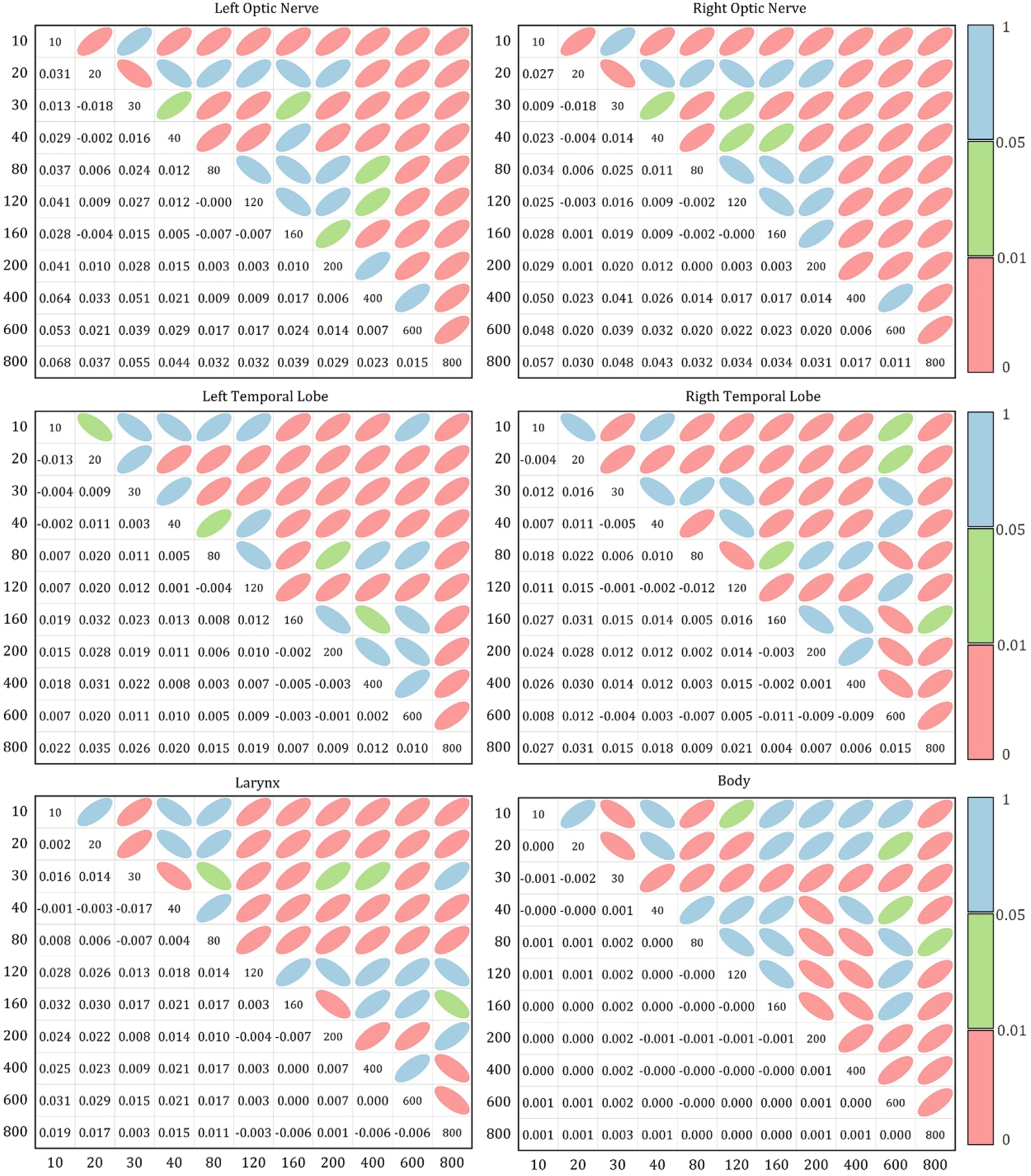
Acknowledgments
This work is supported by the Shanghai Committee of Science and Technology Fund (19DZ1930902, 21Y21900200), Shanghai Xuhui District Artificial Intelligence Medical Hospital Cooperation Project (2020-009), Varian Research Grant (The deep learning based 3D dose prediction and automatic treatment planning).