
Abstract
Purpose. The purpose of this work is to investigate the feasibility of TOPAS-nBio for track structure simulations using tuple scoring and ROOT/Python-based post-processing. Materials and methods. There are several example applications implemented in GEANT4-DNA demonstrating track structure simulations. These examples are not implemented by default in TOPAS-nBio. In this study, the tuple scorer was used to re-simulate these examples. The simulations contained investigations of different physics lists, calculation of energy-dependent range, stopping power, mean free path and W-value. Additionally, further applications of the TOPAS-nBio tool were investigated, focusing on physical interactions and deposited energies of electrons with initial energies in the range of 10–60 eV, not covered in the recently published GEANT4-DNA simulations. Low-energetic electrons are currently of great interest in the radiobiology research community due to their high effectiveness towards the induction of biological damage. Results. The quantities calculated with TOPAS-nBio show a good agreement with the simulations of GEANT4-DNA with deviations of 5% at maximum. Thus, we have presented a feasible way to implement the example applications included in GEANT4-DNA in TOPAS-nBio. With the extended simulations, an insight could be given, which further tracking information can be gained with the track structure code and how cross sections and physics models influence a particle's fate. Conclusion. With our results, we could show the potentials of applying the tuple scorer in TOPAS-nBio Monte Carlo track structure simulations. Using this scorer, a large amount of information about the track structure can be accessed, which can be analyzed as preferred after the simulation.
Export citation and abstract BibTeX RIS

Original content from this work may be used under the terms of the Creative Commons Attribution 4.0 licence. Any further distribution of this work must maintain attribution to the author(s) and the title of the work, journal citation and DOI.
1. Introduction
In the field of radiotherapy and radiation protection, Monte Carlo simulations are a frequently used tool in research and clinical applications (Rogers 2006). However, since Monte Carlo simulations often require very good programming skills, many codes are not suitable for clinical applications, and medical physicists without advanced programming skills. Therefore, the Monte Carlo toolkit TOPAS (TOol for PArticle Simulation) (Perl et al 2012, Faddegon et al 2020) was developed, which makes Monte Carlo simulations more accessible for researchers and clinical users due to its ease of use. The toolkit is based on the already established open access Monte Carlo code GEANT4(Agostinelli et al 2003, Allison et al 2006). This means that TOPAS implies the same physics models and cross section data as GEANT4, but with the difference that the simulations do not have to be written in programming language C++. Simulation geometries, particle sources, scorers, and physics parameters are defined using simple text-based commands. The user can choose from a large variety of predefined options, however, TOPAS can still be used flexibly since advanced users can make use of extensions. Initially, it was applied for proton therapy, but now it can also be used in many other areas of radiation therapy and some medical imaging applications. The tool has already been well-validated against experimental data in previous studies (Perl et al 2012, Testa et al 2013).
Additionally, the TOPAS collaboration has released an extension named TOPAS-nBio (Schuemann et al 2019) (available since August 2019), based on the Monte Carlo Code GEANT4-DNA, for running radiobiology simulations at cellular and sub-cellular scales. For typical clinical applications like dose calculations and dosimetry, simulations are performed on macroscopic scales, while in most cases the condensed history approach is used to reduce computing time. In the condensed history approach, several single scattering events are condensed into one multiple scattering event, while the energy deposition and scattering angle are being determined statistically using corresponding algorithms. The disadvantage of this approach is, however, that it only achieves a reduced spatial resolution of the local deposited energy. In contrast, simulations on small scales like cellular and sub-cellular levels are usually performed using Monte Carlo track structure codes such as GEANT4-DNA to track particles step by step until they reach energies of a few eV. Track structure codes provide the required physics models and precise cross section data, which are not included in conventional codes. Still, this approach is more time consuming than the condensed history approach (Tajik-Mansoury et al 2017). For clinical applications on mm-scales, cut-off energies of 1–10 keV are usually used, whereas for simulations investigating the biological response directly at the DNA or on cellular levels (nm-μm), the particles have to be tracked down to a few eV. For example, electrons with an energy of 10 keV have a residual range in water of ca. 2.5 μm, which is sufficient for macroscopic simulations. However, for simulations on the microscopic level, residual ranges of ca. 3 nm with corresponding electron energies of 20 eV are crucial.
Making use of track structure codes, nanodosimetric quantities like DNA strand breaks and the distribution of ionization clusters can be investigated, which is expected to improve the prediction of the biological effectiveness of heavy charged particle radiation. This might lead to a development of new models of the relative biological effectiveness (RBE) or to the refinement of already existing radiobiological models. In addition to the TOPAS-nBio extension, there is also a microdosimetric extension available focusing on simulations on cellular scales. This extension can be applied to simulate microdosimetric spectra and perform calculations of RBE as well. To calculate microdosimetric quantities, a special microdosimetric scorer is used, which scores each interaction with an energy deposition greater than zero in a corresponding microdosimeter. Contrary to TOPAS-nBio, g4em-standard physics lists are used. Details are described by Zhu et al (2019).
TOPAS-nBio is used to link GEANT4-DNA (Incerti et al 2010a) with TOPAS making new physics lists available in order to simulate track structures down to the eV-regime. Geometry components for biological targets e.g. several DNA models and cellular structures are also accessible in this tool. These are described in detail by McNamara et al (2018). In addition to the simulation of physical interactions, chemical interactions (Karamitros et al 2011) and also biological aspects like DNA repair models (McMahon et al 2016, Warmenhoven et al 2020) can be taken into consideration in order to study the biological damage induced by ionizing particles. Chemical interactions are of particular interest for low-LET radiation since a great amount of damage to the DNA is caused by indirect effects of the radiation such as chemical radicals (Sanche 2012). This toolkit of TOPASbased on the physics lists and chemistry models from GEANT4-DNA has been validated against previous simulation studies and experimental data. This was done by comparing the prediction of DNA damage in different geometries to measurement data and previously performed simulation studies (McNamara et al 2017). More studies have already been published investigating TOPAS-nBio for nanodosimetric simulations showing the potential of this extension. Zhu et al (2020) investigated the effect of different physics and chemical models in TOPAS-nBio on the yield of the single strand break (SSB) and double strand break (DSB) in proton simulations. Furthermore, in a study by Hahn and Villate (2021), the extension was used to determine the effect of different geometric models of the distribution of nanoparticles within a cell in simulations using gold nanoparticles for dose enhancement by simulation the radioactive decay of 198Au and focusing on the deposited energy of different cell organelles.
With the release of GEANT4-DNA, the example repertoire of GEANT4was extended with eleven examples considering track structure simulations with GEANT4-DNA, which are described and analyzed in detail by Incerti et al (2018) (hereinafter Incerti2018). These simulations include the examples dnaphysics, range, spower, mfp, and w value, which will be further specified in sections 2.1.1–2.1.5. In TOPAS-nBio, these examples are not in any way pre-programmed and the corresponding values of those examples cannot be scored directly. In the first part of this research, the main focus was to investigate the feasibility of performing these example simulations in TOPAS-nBio. We present a solution to determine the physical properties by taking advantage of the tuple scorer, which stores detailed tracking information of track structure simulations in one single output file. Using this method, a high programming effort is avoided. We intended to re-simulate especially the five examples tnat were investigated by Incerti2018 with TOPAS-nBio since they are often used as key quantities for evaluating track structure codes. Further, to validate this model, simulation results using TOPAS-nBio were compared to those performed with the pre-programmed examples in GEANT4-DNA.
In a second part, further applications of the TOPAS-nBio tool were investigated, focusing on physical interactions and deposited energies of electrons of low energies in the range of 10–60 eV. This energy range was chosen since the most probable energy of secondary electrons produced by a primary ion of clinically relevant energies is approximately 10 eV and the mean energy is about 50–60 eV (Pimblott and LaVerne 2007). By using the tuple scorer, the individual fate of each electron could be examined and analyzed in detail.
2. Materials and methods
2.1. GEANT4-DNA example applications
At the beginning of this section, we will briefly introduce the examples that were re-simulated during this study and previously carried out with GEANT4-DNA by Incerti2018. All simulations were performed in liquid water. Details such as simulation parameters will be further discussed in the following subsections.
2.1.1. Dnaphysics example
The occurrence of various electron, proton, and hydrogen processes is counted from a total of 100 primary protons with an initial energy of 100 keV.
2.1.2. Range example
The energy-dependent range r of one particle is determined as the sum of all step lengths between two interaction points. The step length is calculated using the three-dimensional Pythagorean theorem and the coordinates x, y, z of each trajectory point s:

where Ns is the maximum step number.
2.1.3. Spower example
The energy-dependent stopping power s of the particles is studied. For this purpose, the sum of the deposited energy Es of each step s per primary particle is divided by the corresponding range r (see above):

2.1.4. Mean free path (Mfp) example
The mfp is the average length of the first step of a particle with a certain kinetic energy. The inelastic mean free path (imfp) is the average length of the first step of a particle considering only inelastic interactions, in which case elastic interactions are not simulated. Since the coordinates of the first trajectory point are located in the origin, this results in the following expression:

Here N is the number of events e. This equation is also valid for the calculation of the imfp.
2.1.5. W value example
The W-value w is determined by the ratio of the initial particle energy E and the mean number of ionizations  per event:

2.2. Simulations of GEANT4-DNA example applications using TOPAS-nBio
In the simulations performed with TOPAS (Perl et al 2012), we used TOPAS version 3.2.p2, which is based on the GEANT4version 10.05.p01. The features of TOPAS-nBio are made accessible by several extensions provided by the TOPAS collaboration. We used TOPAS-nBio v1.0-beta.1. Even though the latest GEANT4 version (GEANT4 10.07) is already released, there is no disadvantage of running the simulations based on GEANT4 version 10.05, as there are no significant differences when comparing the example results from those two different GEANT4 versions as shown in the appendix.
Most of the necessary simulation parameters, such as those concerning geometry and radiation source, are described in Incerti2018 and could thus be easily adapted in the TOPAS simulations. All remaining parameters were extracted from the simulation files provided on GitHub 5 by the GEANT4 collaboration. These are summarized in table 1. In each simulation, except of the dnaphysics example, an isotropic particle source was placed at the center of a sphere with a radius of 1 m. This was filled with liquid water (G4_WATER) since cross sections data in GEANT4-DNA are only available for liquid water and DNA-related materials. Using G4_WATER, water has a density of 1.0 g cm−3 and a mean ionization potential of IW = 78 eV. In the dnaphysics example application the particle source was placed in the middle of a box with an edge length of 100 μm. The physics lists G4EmDNAPhysics_option2, G4EmDNAPhysics_option4 and G4EmDNAPhysics_option6 were used in separate runs for all simulations concerning electrons. Simulations for protons and alpha particles in the range example were performed using G4EmDNAPhysics_option2. For a correct calculation of the stopping power of electrons, G4EmDNAPhysics_stationary_opt2, G4EmDNAPhysics_stationary_opt4 and G4EmDNAPhysics_stationary_opt6 needed to be used, since here the kinetic energy of the particle is constant in each step as described by Incerti2018. In most simulations the default tracking cut of the particles was applied; details are listed in table 1. The number of primary particles was set between 102 and 104 depending on the particle type and example application similar to Incerti2018. In the mfp example, the mfp was once investigated including all electron processes and a second time considering only inelastic interactions (imfp) as done by Incerti2018. For the calculation of the imfp, we used a physics list adopted from TsEmDNAPhysics, so that elastic interactions could be inactivated. All other physics models and processes were implemented as it is the case in G4EmDNAPhysics_option2, G4EmDNAPhysics_option4, and G4EmDNAPhysics_option6 which is specified in table 2.
Table 1. Overview of the relevant simulation parameters applied in the different examples in this study using TOPAS-nBio.
| Dnaphysics | Range | Spower | Mfp | W value | |
|---|---|---|---|---|---|
| Geometry | TsBox | TsSphere | TsSphere | TsSphere | TsSphere |
| with edge length | r = 1 m | r = 1 m | r = 1 m | r = 1 m | |
| of 100 μm | |||||
| Material | G4_WATER | G4_WATER | G4_WATER | G4_WATER | G4_WATER |
| Source | Particle type: p | Particle type: e-, p, α | Particle type: e- | Particle type: e- | Particle type: e- |
| Particle energy: | Particle energy: | Particle energy: | Particle energy: | Particle energy: | |
| 100 keV | e-: 10–106 eV | e-: 10–106 eV | 10–106 eV | 10–105 eV | |
| p: 103–106 eV | |||||
| α: 103–106 eV | |||||
| Physics lists | g4em-dna_opt2/4/6 | g4em-dna_opt2/4/6 | g4em-dna- | g4em-dna_opt2/4/6, | g4em-dna_opt2/4/6 |
| stationary_opt2/4/6 | TsEmDNAPhysics2 a | ||||
| Transport | Tracking cut: | Tracking cut: | Tracking cut: | Tracking cut: | Tracking cut: |
| Parameters | default b | e-: 10 eV | default b | default b | default b |
| p: 400 eV–3 keV c | |||||
| α: 1 keV | |||||
| MaxStepNumber: | MaxStepNumber: | MaxStepNumber: | MaxStepNumber: | MaxStepNumber: | |
| default d | default d | 1000 | 1 | default d | |
| Scoring | TupleAll e | TupleAll e | TupleAll e | TupleAll e (all) | pTuple |
| Process name | EventID | EventID | pTuple (inel.) | EventID | |
| Deposited energy | Only primary particles | EventID | Process name | ||
| only primary particles | |||||
| Histories in | 102 | e-: 103 | 104 | 104 | 104 |
| Run | p, α: 102 |
a
Extension adapted from TsEMDNAPhysics to inactivate elastic scattering. Models for the different processes were selected according to the dna physics list options.
b
Default tracking cut for e-: opt2 = 7.4 eV, opt4 = 10 eV, opt6 = 11 eV, for p,  = 100 eV, for α = 1 keV.
c
The tracking cut was set to 400 eV at initial proton energies of 1 keV and to 3 keV for initial energies greater than or equal to 500 keV. For all intermediate energies the tracking cut was interpolated logarithmically.
d
Default MaxStepNumber = 106.
e
Extension adapted from pTuple-Scorer, but modified so that all processes (also those with edep = 0
= 100 eV, for α = 1 keV.
c
The tracking cut was set to 400 eV at initial proton energies of 1 keV and to 3 keV for initial energies greater than or equal to 500 keV. For all intermediate energies the tracking cut was interpolated logarithmically.
d
Default MaxStepNumber = 106.
e
Extension adapted from pTuple-Scorer, but modified so that all processes (also those with edep = 0  elastic scattering) are included.
Table 2. Settings of the physics models used for the simulation of the imfp so that they correspond to the physics lists G4EmDNAPhysics_option2/4/6. Elastic scattering is switch off, since only inelastic interactions are taking into account when calculating imfp. Electron solvation does not need to be specified since it just operates as tracking cut.
| Process | Option 2 | Option 4 | Option 6 |
|---|---|---|---|
| Ionization | Born a | Emfietzoglou b | CPA100 c |
| Excitation | Born a | Emfietzoglou b | CPA100 c |
| Attachment | True | False | False |
| Vibrational excitation | True | False | False |
| Elastic scattering | False | False | False |
a Incerti et al (2010b). b Kyriakou et al (2015). c Bordage et al (2016).
Contrary to GEANT4, the simulations are not pre-programmed in TOPAS, and the results are not directly obtained after running the simulation as it is the case in GEANT4. In order to still be able to calculate these corresponding quantities, we used the tuple scorer in our simulations. This scorer stores information related to a particle track such as the particle type and the x-, y- and z-position of the trajectory step point in one file. In addition, the user can decide whether additional tracking information should be included in the output file by selecting items from the following list:
- EventID (number of the primary particle)
- TrackID (identification number to differentiate between tracks of primary and secondary particles)
- Step number (number of the step of the corresponding track)
- Particle name
- Process name
- Volume name
- Volume copy number (copy number of a volume, if its geometry is copied in the simulation)
- ParentID (track identification numbers of the parent tracks of chemical reactions)
- Vertex position x/y/z (coordinates of the step points of secondary particle tracks in relation to their origin)
- Global time (time of flight)
- Energy deposited
- Kinetic energy (before interaction)
The respective quantity of each example could then be calculated from the corresponding tracking information. For some simulations, it was also useful to add filters to the scorers, e.g. when focusing exclusively on primary particles or particles of a given type. This can be a helpful feature, for example, to keep the output files small and to simplify and speed up the analysis. An overview of possible scoring filters is provided on the TOPAS documentation website 6 by the TOPAS collaboration. The tuple scorer provided by TOPAS does only account for interactions with an energy transfer larger than 0 eV. In order to score elastic scatterings also, the tuple scorer was adapted to score events with an energy transfer of 0 eV. All data were stored in a ROOT file.
To validate our method, simulation results using TOPAS-nBio based on GEANT4 version 10.05 were benchmarked with those of GEANT4-DNA using the same software version. The simulations with GEANT4-DNA were performed using the pre-programmed example files included in GEANT4. When running the simulation files, the user directly receives a file in which the results are listed. Thus, there is no need for additional calculations.
2.3. Extended simulation to investigate the processes of low-energy electrons
The occurrence of physical processes stated in table 3 for electrons of energies between 10 and 60 eV was studied using the physics list G4EmDNAPhysics_opt2. An isotropic source emitting 100 electrons was placed at the center of a cube with an edge length of 100 μm filled with liquid water. The tracking of the particles was terminated by applying the default tracking cut of 7.4 eV. The tuple scorer was applied to investigate detailed track structure information. Post-processing those data, the following investigations were made:
- (i)The frequency of electron processes was investigated by counting each process in total of all 100 primary particles and their secondaries.
- (ii)Since the deposited energy is of particular interest when considering the effect of radiation on DNA scales, this parameter was studied in more detail. The mean deposited energy of a single interaction was calculated per process.
- (iii)Additionally, the sum of the deposited energy of each process per primary particle was calculated.
- (iv)The maximum energy deposited for each process was investigated.
- (v)The chronological order in which the processes of different events and for different initial energies occur along one track was investigated.
Table 3. Brief overview of all possible electron processes included in GEANT4-DNA.
| Process name | Definition |
|---|---|
| Attachment | Electron sub-excitation process; capture of an electron by a electrically neutral molecule, when the kinetic energy is less than the ionization potential and matches the quasibound state of the molecule. OH−, H− and O− ions are produced by the electron interacting with liquid water (Melton 1972, Denifl et al 2012). |
| Elastic scattering | Scattering of the particle interacting with free and bound atoms. In G4EmDNAPhysics_option2 and G4EmDNAPhysics_option4, there is no energy transfer, whereas in G4EmDNAPhysics_option6 a tiny fraction of energy is transferred and the total momentum of the whole system is conserved. |
| Electron solvation | Accumulation of water molecules around a free electron. In GEANT4-DNA, the tracking cut is represented by this process when chemical processes are inactivated. Electrons that reach the tracking cut are then assumed to be solvated (Incerti et al 2018). |
| Electronic excitation | Energy transfer to a bound electron of a molecule with the result that it is excited to a higher energy level. Consideration of the electron excitation states of liquid water. |
| ionization | Detachment of an electron from the electron shell of a neutral atom or molecule, resulting in a positive ion. Taking into account the ionization energies for the valence electrons and the K-shell. |
| Vibrational excitation | Small energy depositions inducing excitation of the vibrational state of the interacting molecule (Michaud et al 2003). Nine excitation phonon modes are taken into account. |
2.4. Analysis of the TOPAS simulations
In order to evaluate the output of the simulations from TOPAS, we used ROOT version 6.20.04, an open-source analysis framework developed and provided by CERN (Brun and Rademakers 1997), and Python 2.7.17. ROOT offers the user the possibility to choose Python for an evaluation of the ROOT files by importing the module root_numpy into Python. More precisely, we used the function root2array for converting a tree, a special structure in a ROOT file containing the stored data, into a numpy structured array. Then, all tracking data could be commonly accessed and processed with Python.
In this study, the corresponding properties were determined in each event individually and then averaged over the complete set of events to determine a mean value and the associated standard deviation. Since no statistical values can be estimated by simulating just one run of the dnaphysics example, the standard deviation was calculated using the results of 20 independent runs performed with different random seeds.
3. Results and discussion
3.1. Simulations of GEANT4-DNA example applications using TOPAS-nBio
3.1.1. Dnaphysics
Figure 1 shows the frequency of individual processes simulated with TOPAS-nBio and GEANT4-DNA using different physics lists. In the bottom panels, the relative deviation from TOPAS-nBio to GEANT4-DNA is visualized. For each process the deviations are smaller than 1.2%. Comparing the counts of each process using G4EmDNAPhysics_opt2, the greatest deviation is 1.2% for electron attachment and the average deviation of all processes using is physics list option 0.2%. Using G4EmDNAPhysics_opt4 and G4EmDNAPhysics_opt6, a maximum deviation of 1.2% and 1.1% respectively is observed for hydrogen excitation. On average the values of TOPAS-nBio and GEANT4-DNA deviate by 0.1% using these two physics lists. However, all values between TOPAS-nBio and GEANT4-DNA coincide within one standard deviation.

Figure 1. Results of the dnaphysics example simulated with TOPAS-nBio (filled bars) and GEANT4-DNA (dashed bars) using three different physics lists. In the lower part of each plot, the percentage deviation between both simulations is shown. Statistical uncertainties of the deviations in the bottom graph are represented by error bars and correspond to one standard deviation.
Download figure:
Standard image High-resolution imageIn addition, figure 2 shows the comparison of the counts per process simulated with TOPAS-nBio using these three physics list options by calculating the percentage deviation between two options. The physics list that is listened first in the legend was always selected as the 'original data'. For example, the calculation of the data series 2 versus 4 was performed as follows:

Here, dp
is the percentage difference of process p,  the counts of process p using physics lists option 2 and
  the counts of process p using physics lists option 4.

Figure 2. Comparison of the results from the textitdnaphysics simulation performed with all three options. When calculating the percentage differences, the physics list option, which is listed in first position in the legend, was set as basis if comparison.
Download figure:
Standard image High-resolution imageThe differences between the individual physics lists are quite low for proton and hydrogen processes since the models of these processes are the same for each physics list option. The deviations are of statistical nature. For electron processes, the absolute differences are between 3.6% and 255%. On average, electron processes deviate by 46% for the different physic list options, thus, the correct choice for simulations in TOPAS-nBio is of great importance since simulation results can differ significantly depending on the applied physics list.
3.1.2. Range
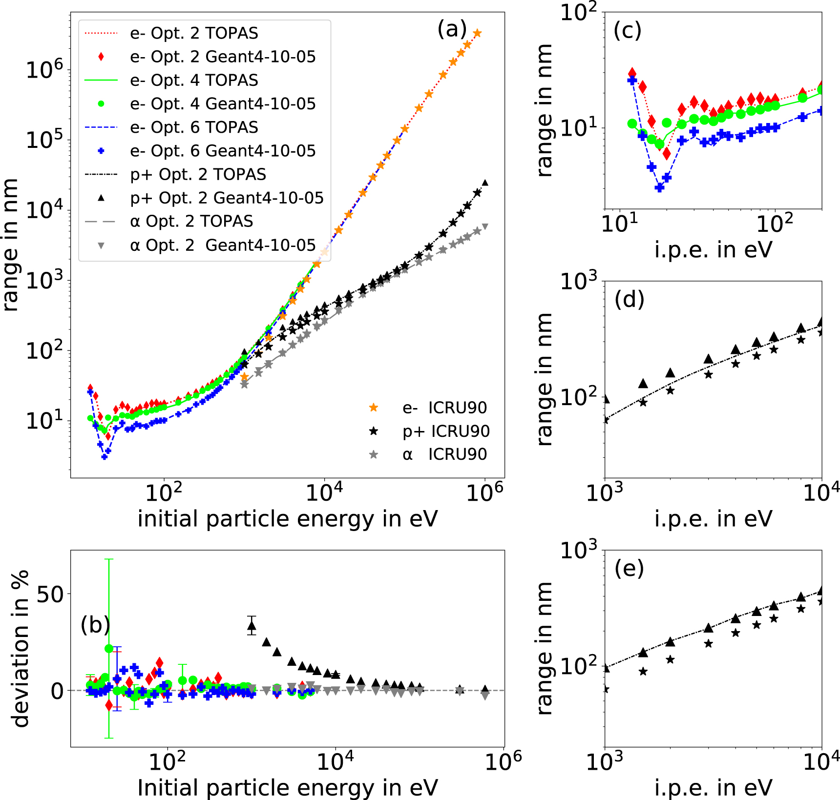
In figure 3(a), the range of the investigated particles is shown as a function of initial energy calculated with TOPAS-nBio and GEANT4-DNA using different physics lists. In TOPAS-nBio, more initial energies were investigated compared to the GEANT4-DNA simulations. Hence, the individual data points produced with TOPAS-nBio are connected by a line to guide the eye. Additionally, the ICRU90 (ICRU 2016) ranges of the particles are illustrated. In figure 3(b), the deviations between the TOPAS-nBio simulations and GEANT4-DNA are portrayed. Considering electrons, large relative deviation can only be observed at small, absolute ranges. For initial electron energies above 500 eV, deviations are smaller than 2%. Regarding option 4, the maximum deviation is slightly above 20%; considering option 2, the deviations range from −7.7% to 14.2%, and using option 6, a maximum deviation of 11.9% at an energy of 40 eV is observed. Nevertheless, the mean deviation for electrons using all three options is statistically disturbed around zero and all deviations are in order of one standard deviation. Here, no systematic deviations can be observed. In figure 3(c), the ranges for electrons of energies from 10 to 100 eV are shown in a zoom-in view. As described by Francis et al (2011), this range profile results from cross sections of inelastic scattering processes implemented in the physics list, which are significantly changing for small energies. This is a consequence of the tresholds for inelastic interactions located in this energy range. By undergoing an inelastic interaction, the particle looses kinetic energy reducing the residual range. Thus, these peaks at lower energies occur as the initial energy exceeds new tresholds for inelastic interactions. Since the tresholds and cross sections of each process differ in the different physics list G4EmDNAPhysics_opt2, G4EmDNAPhysics_opt4 and G4EmDNAPhysics_opt6, the profile of the range at low energies is also different for each simulated physics list.

Figure 3. Results of the range example simulated using TOPAS-nBio and GEANT4-DNA. ICRU90 reference values are shown as well. The visualization of statistical uncertainties in form of error bars on a logarithmic scale might be confusing and hence, they are not depicted in all graphs with logarithmic y-axis. (a) Electron, proton and alpha particle ranges (unzoomed), (b) percentage deviation from the ranges simulated with TOPAS-nBio to the ones with GEANT4-DNA. Statistical uncertainties are represented by error bars for some selected energies exemplarily and correspond to one standard deviation, (c) electron ranges up to 200 eV (zoom-in of (a)), (d) proton ranges between 103 and 104 eV using different tracking cuts. In the simulations using GEANT4-DNA, the default tracking cut was used, whereas in the simulations of TOPAS-nBio a higher, interpolated tracking cut was applied for energies between 1 and 5 keV, (e) proton ranges between 103 and 104 eV using the same tracking cut in both codes (default).
Download figure:
Standard image High-resolution imageWhen comparing the proton ranges in figure 3(d), it is interesting to note that the deviations between TOPAS-nBio and GEANT4-DNA are largest at an initial energy of 1 keV (30%) and then decrease systematically down to a minimum value of 0.6%. These deviations result from the fact that in the GEANT4-DNA pre-programmed examples the tracking cut was not adjusted as described in the study by Incerti2018. In the TOPAS-nBio simulations the tracking cut was set higher resulting in a lower range. Comparing the ranges calculated with TOPAS-nBio and GEANT4-DNA with ICRU90 data, it can be seen that the agreement between TOPAS-nBio and ICRU values is more accurately compared to GEANT4-DNA. For a more accurate comparison between GEANT4-DNA and TOPAS-nBio, the simulations were repeated in TOPAS-nBio, this time using the same tracking cut (100 eV) as in GEANT4-DNA. With this adjustment, the values agree well with those of GEANT4-DNA (see figure 3(e)) and a maximum deviation of 0.6% could be obtained.
The ranges of alpha particles (see figure 3(a)) comply well with both the GEANT4-DNA values and the ICRU values, while deviations are smaller than 3% for all considered energies and coincide within one standard deviation.
3.1.3. Spower
Figure 4(a) shows the mean value of the stopping powers of all three physics list options as a function of the initial particle energy for electrons. Due to practical reasons, only four values were simulated in TOPAS-nBio per physics list. Therefore, the x-axis in 4(a) is discrete and the values of TOPAS-nBio and GEANT4-DNA are plotted side by side for a more concise illustration of the results. While using G4EmDNAPhysics_stationary_opt2 and G4EmDNAPhysics_stationary_opt6 a percentage deviation of 0.12% at maximum of the electron stopping powers is obtained, the deviation for G4EmDNAPhysics_stationary_opt4 is ten times larger with 1.3%. It is noticeable that for G4EmDNAPhysics_stationary_opt2 and G4EmDNAPhysics_stationary_opt6, the stopping powers obtained with TOPAS-nBio are always larger than those from GEANT4-DNA, and contrarily for G4EmDNAPhysics_stationary_opt4, all values from TOPAS-nBio are smaller than those from GEANT4-DNA. However, all values between TOPAS-nBio and GEANT4-DNA agree within one standard uncertainty. For transparency, the uncertainties of the spower example are shown in figure 4(a).

Figure 4. Results of the example applications simulated with GEANT4-DNA and TOPAS-nBio. (a) Spower (b) mfp, (c) imfp and (d) w value. In the bottom graph of each example, the deviation from the results of the examples using TOPAS-nBio relative to GEANT4-DNA is shown. Error bars of some selected, exemplary energies represent one standard deviation. In graphs with a logarithmic scaled y-axis, uncertainties are not portrayed. For the spower example, the x-axis is discrete.
Download figure:
Standard image High-resolution image3.1.4. Mfp
In figure 4(b), the mfp including all processes for electrons is visualized and the imfp is shown in figure 4(c). The difference between TOPAS-nBio and GEANT4-DNA is smaller than 3% for the mfp simulation and 4% at maximum for the imfp simulation. Nevertheless, all values coincide within one standard deviation and no systematic uncertainties can be recognized.
3.1.5. W value
Figure 4(d) shows the W-value as a function of the initial particle energy. The agreement between TOPAS-nBio and GEANT4-DNA is better than 2% for high energies. For smaller energies the deviations can be larger due to the fact that statistical fluctuations are more common since very few interactions occur. In all cases, the deviations are smaller than one standard deviation.
In conclusion, the results obtained with TOPAS-nBio agree well with those generated using GEANT4-DNA. Apart from a few exceptions, deviations are smaller than 5%. All deviations between TOPAS-nBio and GEANT4-DNA are within one standard uncertainty. Hence, the results show that the implementation of the example simulations in TOPAS-nBio as well as the post-processing of the simulation results using ROOT and Python were successful. In addition, it was illustrated that the results vary significantly depending on the used physics list options.
In general, the implementation of the GEANT4-DNA example applications in TOPAS-nBio was easily achievable. Using the tuple scorer, which stores all information relevant to a track in one output file, the user is given the opportunity to evaluate the particle track in a variety of ways. Additionally, this method has the advantage that aspects can be investigated after the simulation that were not considered before since all tracking information are being stored. In case of evaluating the tracking information after a simulation, it must be considered that knowledge of other evaluation programs, in our case ROOT and Python, is required. The implementation of the examples was possible in TOPAS because the user is given the possibility to write own extensions in order to be able to use the entire capacity of GEANT4. In our case, extensions, which are already inserted in TOPAS, could be used as a template, which facilitated the writing of own extensions. In most cases, even just two or three lines had to be edited in the extension files. Probably more complicated extensions could have been written, e.g. to reduce the amount of data or to avoid carrying out a calculation after the simulation, but our goal was to use the simplicity of TOPAS and avoid writing complicated scripts. The amount of data in our simulations was very high because we used the tuple scorer storing all track information. This implies that the more particles are simulated and the more they interact, the larger the file becomes. For example, having a look at the dnaphysics example, the file size for one run using G4EmDNAPhysics_opt2 is around 500 MB. In this file, all tracking information of the 100 primary particles and all particles of further generations are stored step-by-step. If the physics list G4EmDNAPhysics_opt4 or G4EmDNAPhysics_opt6 of the same simulation is used, the output file is smaller, since all in all less interactions occurred (see figure 1).
Altogether, our approach to simulate the examples in TOPAS is simple enough for getting started, however, we recommend to write own extensions according to the quantities, if it is desired to make use of them more frequently.
3.2. Extended simulations regarding the processes of low-energy electrons
In figure 5(a) the frequency of each process in relation to the initial particle energy is illustrated. The most common process for all energies is elastic scattering followed by vibrational excitation. In general, the number of those processes increases with the initial energy, due to the increasing range of the particles noting that in figure 5(a) the y-axis is plotted logarithmically. Both, elastic scattering and vibrational excitation, show a minimal occurrence at an energy of ∼18 eV. Above an energy of 11 eV, the probability of ionization increases since more ionization energy tresholds are exceeded and the related cross sections also increase (Incerti et al 2010b, Bordage et al 2016). The energy tresholds required for an ionization as well as for an electronic or vibrational excitation are listed in table 4. These processes reduce the range and hence the amount of elastic interactions significantly due to a noticeable energy loss. The number of elastic interactions fluctuate further with increasing initial energy because on the one hand, starting with a higher initial energy more interactions, i.e. also usually a greater range, are possible which results in a higher number of elastic interactions. On the other hand, the kinetic energy of the particle and thus the range is reduced since with increasing initial energy more tresholds for inelastic interactions are exceeded and a higher number of inelastic interactions might occur in one event. The electron solvation process operates as a tracking cut because no chemical interactions are taken into account in any simulations. Since secondary particles were also considered in this simulation, more than 100 electron solvations can take place in each simulation with 100 primary particles as with increasing initial energy more secondary particles are being produced. The tracking of those produced electrons is again terminated by this process.
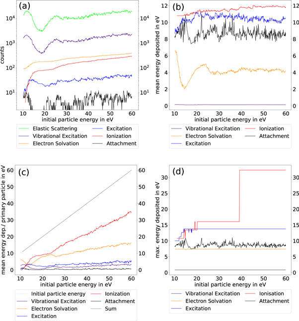
Figure 5. Results of the extended simulations regarding the processes of electrons in the range of 10–60 eV. (a) Frequency of processes from a total of 100 primary electrons including electrons of later generations, (b) mean deposited energy of all primary events of each process, (c) sum of the deposited energy per process in average of all primary electrons, and (d) maximum deposited energy per process. Considering (c) and (d), uncertainties are not shown for a more concise presentation of results. Since ionization only occur above an initial energy of 11 eV, the corresponding results were only plotted for initial energies above this minimum energy.
Download figure:
Standard image High-resolution imageTable 4. Deposited energies in eV by vibrational excitation, electronic excitation and ionization found in our simulations. These energies correspond to the energy tresholds of the associated processes (E
 for vibrational excitation,
  for excitation,
  for ionization) implemented in the different models. The vibrational modes are included in the Sanche Excitation Model described in the study of Michaud and Sanche (1987). The energy tresholds for electronic excitation are taken from the Emfietzoglou Dielectric Model (Emfietzoglou and Moscovitch 2002) and ionization levels are described by Dingfelder et al (1998).
| Vib. mode |

| Electr. excitation level |

| Molecular orbital |

|
|---|---|---|---|---|---|
2( ) ) | 0.835 | A1B1 | 8.22 | 1b1 | 10.79 |

| 0.024 | b1a1 | 10.00 | 3a1 | 13.39 |

| 0.061 | Ryd A + B | 11.24 | 1b2 | 16.05 |

| 0.092 | Ryd C + D | 12.61 | 2a1 | 32.29 |

| 0.204 | Diffuse bands | 13.77 | ||

| 0.417 | ||||

| 0.46 | ||||
 + +
| 0.5 | ||||

| 0.01 |
In figure 5(b) the average deposited energy in one single inelastic interaction is shown as a function of the initial energy separately for each process. For most of the processes, the mean deposited energy remains almost constant over the whole energy range as a consequence of the corresponding energy tresholds (see table 4). The latter is also observed for ionization, which has the highest mean deposited energy in this energy range. Only for electron solvation an energy-dependent mean deposited energy can be observed. The amount of the energy deposition by this process depends on the kinetic energy, which remains after an inelastic interaction if the treshold of 7.4 eV is reached. Since at low energies, only a few eV are left after an ionization or excitation, the mean deposited energy by electron solvation is very small. In figure 5(c), the mean energy deposited in total per primary particle is shown as a function of the initial energy for each process. Those profiles result from the combination of the frequency of each electron process (figure 5(a)) and the corresponding mean deposited energy (figure 5(b)). Altogether, it can be seen that ionization constitutes the largest amount of deposited energy in this energy range.
Figure 5(d) shows the maximum deposited energies for each process as a function of the initial energy. The steps in the line of ionization and excitation visualize the initial energy needed to reach the different tresholds of these processes. The deposited energy always corresponds exactly to the energy tresholds listed in table 4, since the deposited energy in TOPAS-nBio refers to the locally deposited energy, not the kinetic energy loss of the particles. This becomes especially apparent for ionization because the energy tresholds in this case vary the most. Electron solvation results in a maximum deposited energy of 7.4 eV, since this is the tracking cut applied in G4EmDNAPhysics_opt2.
To further examine the interactions of low-energy electrons, the frequency and sequence of different processes were investigated for electrons with an initial energy of 24.2 eV. In figure 6, the number of steps is illustrated as bars with different colors for each process for electrons with an initial energy of 24.2 eV for 100 single events. On a second y-axis, the corresponding range of the electrons is plotted. An electron energy of 24.2 eV was chosen because, on the one hand, particles with this initial energy have sufficient kinetic energy so that all processes occur, and on the other hand, not too many inelastic interactions take place. In figure 6, it can be seen that the more steps occur per event, the larger the range and the more elastic scattering and vibrational excitation takes place. Furthermore, it is noticeable that when two ionizations or excitations appear in one event, the number of steps and the range are small, as it can be observed exemplarily in the zoom-in view. In a further step, the sequence of the processes and the deposition of the energy of individual events were examined. In figure 7, the order of the occurring processes of three different events, which are marked with a red arrow in figure 6, is shown. In this representation, the processes are illustrated as consecutive bars, filled with a different color for each process, and plotted against their corresponding step number on the x-axis. The width of the bars has no further meaning, it only gets smaller the more steps occur in the track. Additionally, the loss of kinetic energy along the steps is shown in each graph.

Figure 6. Step number (bars) and range (x) for 100 events of an energy of 24.2 eV are shown. The number of steps in one event of a process is illustrated in different colors. Events are sorted according to their range. In a zoom-in view, the results of the eleven-events with the smallest range are represented. The red arrows highlight the events that will be examined in more detail in the subsequent part.
Download figure:
Standard image High-resolution image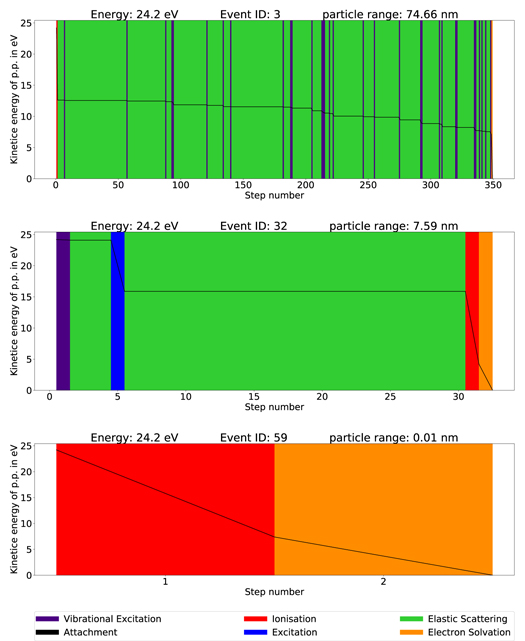
Figure 7. Visualization of three tracks of electrons with an initial energy of 24.2 eV. The process of each step is represented separately by one color and the loss of kinetic energy of the primary particle along each step is also portrayed.
Download figure:
Standard image High-resolution imageBeginning with the track of Event ID 3, the track starts with an ionization, for which reason the particle already loses quite a lot of its kinetic energy. After that, a kinetic energy of only roughly 12 eV is left. This process is followed by a number of elastic interactions alternating with vibrational excitations. The vibrational excitations cause the particle to lose a tiny fraction of its kinetic energy until it reaches the tracking cut of 7.4 eV. The track is then terminated with electron solvation, whereby the remaining kinetic energy is deposited locally. In event 32, the number of steps is significantly smaller and fewer elastic interactions and vibrational excitations are present. However, two additional inelastic processes, ionization and excitation, occur for this purpose through which the particle loses a lot of kinetic energy simultaneously. It is also typical for particles in this energy regime that if there are two inelastic interactions (except of vibrational excitations) in one event, the second one occurs at the end of the track. In this case, the remaining kinetic energy is smaller than the tracking cut, which means that the energy is deposited locally by electron solvation as a last step of the track.
In addition to these two characteristic histories of a particle with an initial energy of 24.2 eV, in Event ID 59, the particle reaches the tracking cut already after having conducted only one step. Such a scenario is only possible if ionization occurs as the first process and such a large amount of energy is transferred to the secondary particle that the residual energy of the primary particle is smaller than the tracking cut. Since in most cases only small fractions of kinetic energy are transferred to secondary particles, this kind of track is rather unlikely.
In conclusion, the simulations regarding electrons of energies between 10 and 60 eV showed that the most frequent process is elastic scattering, while the largest amount of energy is deposited by ionization. Thus, the selection of the correct model for ionization is very important for simulations on molecular levels and for DNA damage studies, and should therefore be well considered. The models vary with the different physics lists and can also be selected independently in TOPAS using TsEmDNAPhysics. The model of the processes could not be validated yet due to the absence of experimental data below 1 keV. However, this investigation should give an insight of how damage on molecular levels and DNA is produced. Especially, when further simulations are made with these models to determine, for example, the distribution and amount of SSB and DSB in relation to the effect of radiation at biological levels.
4. Conclusion
Examples pre-programmed in GEANT4, addressing the possibilities of GEANT4-DNA, were coded and re-simulated in TOPAS-nBio to check the feasibility and handling of the toolkit TOPAS. The tuple scorer can be used for further post-processing the tracking information in order to calculate corresponding variables or to carry out detailed investigations of the particle track. A comparison of the original results with GEANT4-DNA showed that the implementation of the GEANT4-DNA example applications in TOPAS-nBio was successful, as deviations in the results of the examples were less than 5.6% in most cases. Furthermore, no significant deviations could be observed. In TOPAS, not always the latest version of GEANT4 is available. However, running the simulations with TOPAS based on GEANT4 version 10.05 shows no significant differences in comparison to simulations performed with GEANT4 version 10.07. The extended simulations provided an insight into the step-by-step interactions of electrons with initial energies between 10 and 60 eV. Using the tuple scorer, it could be shown that in this energy range, the largest part of the energy is deposited by ionizations which influences a particle's fate with respect to its range and the frequency of other occurring processes.
The project was supported by the Federal Ministry of Education and Research within the scope of the grant 'Physikalische Modellierung für die individualisierte Partikel-Strahlentherapie und Magnetresonanztomographie', (MiPS, grant number 13FH726IX6).
Appendix
Although there is no indication in the release note of version 10.06 and 10.07 that the results concerning our simulations would be affected by the update from version 10.05 to version 10.07, we wanted to ensure that the simulations with TOPAS-nBio based on GEANT4 version 10.05, do not lead to significantly different results than with the current GEANT4 version 10.07. Therefore, the examples simulated in GEANT4 10.05 were additionally compared with the simulation results of the current version published on GitHub. For this purpose, the simulations of the example applications were run exactly as they are included in GEANT4 to make sure that all simulation variables are the same. Results could not be compared for all simulations as described in table 1 since only a selection of calculated data is available on GitHub. The dnaphysics example could not be compared with our GEANT4-DNA results since the data are not available on GitHub (probably due to the large amount of data).
As it can be seen in figure A1, the results of both different GEANT4 versions agree well for all simulated examples. In the range simulation, deviations are generally smaller than 5%, except of some individually cases. Considering all other examples, deviations are well below 1%. All deviations are distributed around 0 which proves that these are of statistical nature and not of a systematic deviation.

Figure A1. Comparison of the investigated examples simulated with GEANT4 10.07 and GEANT4 10.05: (a) range, (b) spower, (c) mfp and (d) w value. In the simulations electrons and the physics constructor G4EmDNAPhysics_option2 were used. The w value example was excluded. In this case the physics constructor G4EmDNAPhysics_option4 was used. Uncertainties are smaller than the symbol size and therefore not illustrated. In the bottom graph of each example, the deviation of the simulations using GEANT4 10.05 relative to GEANT4 10.07 are illustrated.
Download figure:
Standard image High-resolution image
In conclusion, this comparison of the two software versions confirmed that no parameters in the physics lists concerning these simulations changed due to the update. Therefore, there is no disadvantage in simulating the examples for a more detailed comparison with TOPAS3.2 based on GEANT410.05.
Footnotes
- 5
- 6