

Abstract
Proton therapy is very sensitive to daily density changes along the pencil beam paths. The purpose of this study is to develop and evaluate an automated method for adaptation of IMPT plans to compensate for these daily tissue density variations. A two-step restoration method for 'densities-of-the-day' was created: (1) restoration of spot positions (Bragg peaks) by adapting the energy of each pencil beam to the new water equivalent path length; and (2) re-optimization of pencil beam weights by minimizing the dosimetric difference with the planned dose distribution, using a fast and exact quadratic solver. The method was developed and evaluated using 8–10 repeat CT scans of 10 prostate cancer patients. Experiments demonstrated that giving a high weight to the PTV in the re-optimization resulted in clinically acceptable restorations. For all scans we obtained V95% ⩾ 98% and V107% ⩽ 2%. For the bladder, the differences between the restored and the intended treatment plan were below +2 Gy and +2%-point. The rectum differences were below +2 Gy and +2%-point for 90% of the scans. In the remaining scans the rectum was filled with air, which partly overlapped with the PTV. The air cavity distorted the Bragg peak resulting in less favorable rectum doses.
Export citation and abstract BibTeX RIS
Introduction
Intensity-modulated proton therapy (IMPT) allows for highly localized dose delivery, but is also sensitive to inter-fraction variations in the location of the Bragg peak (Lomax 2008a, 2008b). Such variations can be induced by variations in the tissue density along the pencil beam path for example caused by changes in organ filling or by relative movements of organs, and may cause large discrepancies between the planned and delivered dose distribution (Kraan et al 2013). A strategy to prevent this passively is the generation of robust treatment plans (Li et al 2015). This strategy can, however, lead to increased doses to organs at risk (OARs) (Van de Water et al 2016). Ideally, adapting for the variations at time of treatment should be sub-minute after imaging. This is currently not feasible using normal treatment planning workflow, where a full treatment plan is generated from scratch.
This study is part of a project which aims to reduce the time for a re-optimization of the treatment plan by greatly simplifying the optimization problem. The approach is to create in the treatment planning phase an individualized library-of-plans for possible patient anatomies capturing relatively large inter-fraction organ motion. The library can be derived from the patient's planning CT scans or a population-based statistical model describing anatomy variations (Bondar et al 2012, Heijkoop et al 2014). Just prior to each treatment fraction and based on in-room volumetric imaging, the treatment plan that best fits the anatomy-of-the-day will be selected for delivery. Density changes along the beam paths will in general still occur, and need to be corrected, which is the topic of this study. Because generating fully optimized treatment plans for prostate cancer patients as described below takes on average about 25 min, a full optimization is not possible. Therefore we focus on correction for density changes only. The aim of this study is to develop and evaluate a re-optimization method that quickly and automatically restores a proton therapy dose distribution that has been distorted by density changes along the path of the beams. Applying this restoration method right before treatment is a step towards online-adaptive IMPT. The use of the restoration method is not exclusive to library-of-plans strategies but can also be applied to a static treatment plan to mitigate the impact of daily density changes. In this latter case, it would be assumed that (moderate) inter-fraction organ motion is accounted for by a margin around the clinical target volume (CTV).
Zhang et al (2011) also investigated a procedure to restore the planned dose to the prostate. In this procedure, the energy of every proton beam is adjusted according to the new water equivalent path length (WEPL) calculated from the daily CT scan. The intensities of the proton pencil beams remained as planned. The method was tested on a phantom prostate patient, for which they assumed that the prostate would only shift rigidly inside the phantom from fraction to fraction. Two treatment techniques were evaluated; one using distal edge tracking (DET), a type of IMPT placing spots only at the distal edge of the target, and one using 3D IMPT (which in this paper is abbreviated to IMPT), where spots are placed in the whole target volume. Effectiveness of this method was evaluated by comparing the adapted and non-adapted dose distributions for both treatment types. Good restorations were achieved for the DET plans, but the method did not work for IMPT plans, which is currently considered as the state-of-the-art treatment technique.
In our restoration method we also start with WEPL correction, but we proceed with a re-optimization of the pencil beam weights. Evaluations were performed using CT scans of 10 patients. Four re-optimization methods have been compared to find the one resulting in the best restorations. For all patients we checked whether these restorations indeed resulted in clinically acceptable dose distributions and recorded the re-optimization time.
Methods and materials
Patient data
For the 10 study patients we had a planning CT scan taken with contrast and 8–10 repeat CT scans without contrast available, which were acquired during the course of a fractionated photon radiotherapy treatment. To avoid that the results would be perturbed by artificial density changes caused by the contrast we ignored the planning CT scan and used the first repeat CT scan as planning CT scan in this study. A total of 80 repeat scans were used. In each scan, the prostate, seminal vesicles, and lymph nodes were delineated as target structures. The delineated OAR in the planning CT were the rectum, bladder, small and large intestines, and the femoral heads.
Treatment planning
Dose was prescribed according to a simultaneously integrated boost scheme in which the high-dose PTV (prostate + 4 mm margin) was assigned 74 Gy and the low-dose PTV (lymph nodes and seminal vesicles + 7 mm margin) 55 Gy, to be delivered using two laterally opposed beams. We selected this treatment group for evaluation as a theoretical benefit of proton therapy has been demonstrated for the treatment of larger volumes associated with advanced-stage disease (Widesott et al 2011). Note that in this study we used for each patient, instead of a library-of-plans, a static treatment plan with tight CTV-to-PTV margins that were supposed to account for inter-fraction geometrical errors due to internal organ motion, but not to account for density changes along the paths of the pencil beams. The latter will be accounted for by the dose restoration method proposed in this study. The PTV-intermediate is a 15 mm transition region between the expanded prostate and the expanded lymph nodes and seminal vesicles and was added to obtain the desired dose fall-off. The PTV-low consists of the expanded seminal vesicles and lymph nodes, excluding the transition region. To achieve the dose fall-off outside the target areas, conformity rings were created (see figure 1).
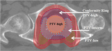
Figure 1. The PTV-high is an expansion of the prostate. The PTV-intermediate is a 15 mm transition region between the high-dose and low-dose PTV. The PTV-low consists of the expanded seminal vesicles and lymph nodes, excluding the transition region. The PTV-full consists of the PTV-high with a 15 mm expansion and PTV-low. The conformity ring around the PTV-high is the PTV-full excluding the PTV-low. The red area represents the 0–10 mm conformity ring of PTV-full.
Download figure:
Standard image High-resolution imageAll IMPT plans were generated using 'Erasmus-iCycle', our in-house developed treatment planning system for fully automated plan generation (Breedveld et al 2012, Van de Water et al 2013), combined with the 'Astroid' dose engine (Kooy et al 2010). Erasmus-iCycle uses a multi-criteria optimization to generate a clinically desirable Pareto optimal treatment plan on the basis of a wishlist consisting of hard constraints and objectives (see table 1). This wishlist is created by physicians and is often used for the entire patient group (i.e. all prostate cancer patients). Constraints are never violated in the plan generation. Based on their assigned priorities, the objective functions are minimized sequentially. The achieved objective value is set as an additional hard constraint that has to be respected during the minimization of the lower priority objective functions (lexicographic optimization). More details on Erasmus-iCycle can be found in Breedveld et al (2009, 2012), Van de Water et al (2013, 2015) and Voet et al (2012). The wishlist used for plan generation in this study is shown in table 1, combined with figure 1. More details about the use of a wishlist are given in Breedveld et al (2009). Generating treatment plans using Erasmus-iCycle with this wishlist takes on average about 25 min.
Table 1. The 'wishlist' with planning constraints and objectives used for automated IMPT plan generation. Constraints will always be met. The priority numbers of the objectives indicate the order in which objectives are to be optimized. A low number corresponds to a high priority. The PTV structures are shown in figure 1. The objectives with priorities 4–8 were assigned a limit of 1 Gy in order to obtain very low dose values while at the same time not imposing an impossible goal.
| Constraints | Structure | Type | Limit |
|---|---|---|---|
| PTV-high | Minimum | 0.97 × 74 Gy | |
| PTV-intermediate | Minimum | 0.99 × 55 Gy | |
| PTV-low | Minimum | 0.99 × 55 Gy |
| Objectives priority | Structure | Type | Limit |
|---|---|---|---|
| 1 | PTV-high | Maximum | 1.07 × 74 Gy |
| 1 | PTV-intermediate | Maximum | 1.07 × 74 Gy |
| 1 | PTV-low | Maximum | 1.07 × 55 Gy |
| 2 | Conformity ring PTV-high | Maximum | 1.07 × 74 Gy |
| 2 | Conformity ring PTV-full 0–10 mm | Maximum | 1.07 × 55 Gy |
| 2 | Conformity ring PTV-full 10–15 mm | Maximum | 0.90 × 55 Gy |
| 3 | Femoral heads | Maximum | 50 Gy |
| 4 | Rectum | Mean | 1 Gy |
| 5 | Small and large intestines | Mean | 1 Gy |
| 6 | Bladder | Mean | 1 Gy |
| 7 | Femoral heads | Mean | 1 Gy |
| 8 | All conformity rings | Mean | 1 Gy |
| 8 | All conformity rings | Maximum | 1 Gy |
| 9 | Total spot weight | Sum | 1 Gp |
Abbreviations: PTV = planning target volume; Gp = Gigaprotons.
To investigate the performance of the dose restoration method developed in this study, the intended treatment plans were generated without including patient setup and range robustness in the optimization. If the restoration method works well, the degree of robustness included in the treatment plan can be reduced, as the coverage loss due to density changes can be mitigated by our method of dose restoration. Reducing the degree of robustness, is expected to reduce the dose in OARs (Van de Water et al 2016).
Dose restoration
The proposed restoration method assumes that a repeat CT scan acquired just prior to dose delivery is available and that the prostate is aligned to the treatment beams by a couch translation using implanted intra-prostatic markers. The restoration method takes this image-guidance procedure into account by aligning each repeat CT scan to the planning CT using the implanted markers. Furthermore, we take as a starting point that repeat CT scans do not have automatically or manually delineated contours, meaning that only the structures projected from the planning CT to the repeat CT scans, i.e. the projected planning structures, are available for the re-optimization (see figure 2, middle). The proposed restoration method restores the dose for all voxels of the structures that are used in the full optimization and hence are mentioned in the wishlist (see table 1). For these voxels the dose deposition matrices are required as these matrices hold the dosimetric effect of every pencil beam to every selected voxel. Multiplied with the pencil beam weights this obtains the dose distribution in these selected voxels. For the planning CT with the planning contours, the matrices are already initialized due to the full optimization, using the energies chosen during optimization. As the dose deposition matrices depend on the path towards the voxels and the energies of the pencil beams, they need to be recalculated for the new paths based on the repeat CT scan with the projected planning contours. When the pencil beam energies are changed during restoration, the matrices need to be recalculated once more. Voxels of structures that are not included in the wishlist, i.e. which are not used in the full optimization, are therefore not included in the restoration to limit the calculation time. The order of importance of the structures of the planning CT scan, i.e. the planning structures, can be used to adjust the weight or importance factor of specific voxels in the re-optimization in order to improve the results. The advantage of this methods is that it does not require a time-consuming contouring step and can immediately commence after the alignment of the repeat CT scan to the planning CT scan. The definition of these importance factors is given in the next section.
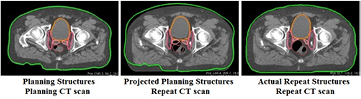
Figure 2. This study uses three combinations of CT scans and contour sets. Left: a planning CT scan with structures contoured in the planning CT scan. Middle: a repeat CT scan with structures projected from the planning CT to the repeat CT scan. Right: a repeat CT scan with structures contoured in the repeat CT scan.
Download figure:
Standard image High-resolution imageThe proposed restoration method consists of two steps. In the first step the spot positions (Bragg peaks) are restored by adapting the energy of each pencil beam such that the coordinates of the Bragg peaks in the planning CT scan and in the repeat scan are equal. Pencil beam directions remain unchanged. Figure 3 shows a schematic representation of this procedure. The result of this step is the energy-restored dose distribution.

Figure 3. Restoring spot positions. Left: the spot positions as intended. Middle: an air cavity causes a displacement and deformation of the upper spot. Right: The energy of the pencil beam has been adapted to restore the spot position. Note that the restoration of spot positions does not adapt for changes in shape and location of the target. If the target shows large geometric changes, the energy-restored spots will not necessarily end up in the target.
Download figure:
Standard image High-resolution imageRestoring the Bragg peak changes its intensity and shape. Hereto we require to re-optimize the pencil beam weights to match the intended dose as much as possible. The change in shape depends on the structures and air cavities along the pencil beam path. Figure 4 illustrates the change in shape when a pencil beam moves fully (middle) or partly (bottom) through an air cavity. We will refer to the changed Bragg peaks as distorted Bragg peaks.
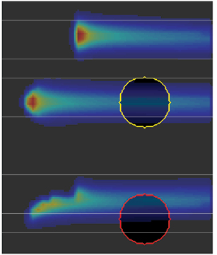
Figure 4. When a pencil beam moves through an air cavity, the shape of the Bragg peak changes.
Download figure:
Standard image High-resolution imageDue to the changes in intensity and shape due to the energy-restoration, the dose deposition matrices need to be recalculated prior to the pencil-beam re-optimization. Instead of a full multi-criteria optimization as used for generation of the intended dose distributions with Erasmus-iCycle, the differences between the actual and intended dose distribution are used to define a quadratic objective function. This objective function contains all structures that are included as constraints or objectives in the wishlist. This re-optimization method uses the BOXCQP algorithm (Voglis and Lagaris 2004, Breedveld et al 2006).
The quadratic objective function is given by

Here  is the actual dose, calculated as the product of the dose deposition matrix
  and the spot-weight vector
  . At the start of a pencil beam weight re-optimization,
  is the energy-restored dose (see above),
  is the intended dose.
  is a diagonal matrix containing importance factors of the voxels (see below).
  is a smoothing term that is also further explained below.
The quadratic objective function can be written in canonical form as

where
More information on these equations can be found in Breedveld et al (2006). The smoothing term  was introduced to keep the Hessian
  positive definite at all times. Without this term the Hessian is not positive definite when for instance the same dose can be achieved in two different ways. This can happen if two similar proton spots are included in the treatment plan. A simple approach which changes the solution minimally is to take
  small (
 ) and
) and  the identity matrix.
The BOXCQP algorithm searches for the optimal spot-weight vector f by minimization of the function s( f).
Assignment of voxel importance factors in s( f) (equations (1) and (2))
Four different approaches for assigning importance factors to the voxels were evaluated. Table 2 contains the details of the different approaches. Approaches B–D could be applied with 1–5 iterations (denoted as B1–B5, C1–C5 and D1–D5), yielding a total of sixteen different re-optimization methods.
Table 2. Overview of the investigated approaches for assignment of voxel importance factors.
| Method A (1 iteration) | All voxels in the structures in the wishlist (table 1) have importance factor 1 throughout the re-optimization;  is the identity matrix is the identity matrix |
| Method B (1–5 iterations) | In the first iteration all voxels in the targets have importance factor 1000. The other voxels have factor 1. In each subsequent iteration the dose distribution is evaluated. Target voxels receiving either too little or too much dose, i.e. less than 95% or more than 107% of the prescribed dose, will get their factor doubled |
| Method C (1–5 iterations) | All voxels in the targets have importance factor 1000. In the remaining structures the dose is evaluated. All voxels in the structure receiving the highest dose get a factor 500. In every iteration the next structure receiving the highest dose also gets factor 500. Each structure can only be selected once |
| Method D (1–5 iterations) | In every iteration the difference between the intended dose and the actual dose is determined for each structure. The structure with the highest mean difference will get a factor 1000 for every voxel. In every iteration a new structure with factor 1000 is added |
Evaluation and comparison of intended and restored plans
All intended and restored treatment plans were evaluated by visual inspection of the dose distributions, the DVHs of the target volumes and OAR, and the clinical constraints. Visual inspection of the restored dose distribution was used to check for hotspots. For the PTV and CTV structures (see table 1), we report the V95% and V107%. The rectum was evaluated using the Dmean, V45 Gy, V60 Gy and V75 Gy, and the bladder using the Dmean, V45 Gy and V65 Gy.
For evaluation of the restored dose distribution, both the projected planning structures and the actual repeat structures were used. First we evaluated the restored dose distribution on the projected PTV and the actual repeat CTV. Secondly, the restored dose distribution was evaluated on the projected OARs and the actual repeat OAR. Besides the evaluation of the obtained treatment plans, the calculation times of the restoration methods were compared.
Results
Distortion for the projected planning structures due to density changes
Figure 5 shows boxplots depicting the differences of the distorted dose distribution in the repeat CT scans minus the intended dose distribution of the planning CT scans for all 80 repeat CT scans. The differences are calculated for the projected planning structures showing the starting point for dose restoration. For all scans the target coverage deteriorates due to the density changes, whereas the OARs dose remain similar on average.
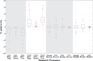
Figure 5. Box plots depicting the difference in dosimetric parameters of the distorted minus the intended dose distributions for all 80 scans based on the projected planning structures. Each box plot indicates the median and the 25th and 75th percentiles of the obtained differences. The dashed lines depict the remaining differences which are not outliers. Values are defined outliers if they are more than 1.5 times the distance between the 25th and 75th quartiles away from the quartiles. The red marks indicate the outliers.
Download figure:
Standard image High-resolution imageResults for projected planning PTV of all restoration methods
The intended treatment plans were optimized to ensure that at least 98% of the volume of the PTV structures given in the wishlist (table 1 and figure 1) receives 95% of the prescribed dose and no more than 2% of the volume receives more than 107%. For the result of the restoration method to be clinically acceptable, we required that these objectives should still be met for 98% of the scans (i.e. for 98% of the scans V95% ⩾ 98% and V107% ⩽ 2%). Table 3 shows the percentage of the scans for which V95% ⩾ 98% and V107% ⩽ 2% for the intended and distorted treatment plans as well as for each restoration method.
Table 3. Percentages of the 80 dose distributions that meet the target constraints for the investigated restoration methods based on the projected planning structures.
| V95% ⩾ 98% PTV-high | V95% ⩾ 98% PTV-interm. | V95% ⩾ 98% PTV-low | V107% ⩽ 2% PTV-high | V107% ⩽ 2% PTV-interm. | V107% ⩽ 2% PTV-low | |
|---|---|---|---|---|---|---|
| Intended | 100.0 | 100.0 | 100.0 | 100.0 | 100.0 | 100.0 |
| Distorted | 45.0 | 77.5 | 31.3 | 45.0 | 91.3 | 0.0 |
| Energy-restored | 77.5 | 95.0 | 58.8 | 33.8 | 95.0 | 0.0 |
| A | 100.0 | 98.8 | 93.8 | 90.0 | 100.0 | 6.3 |
| B1 | 100.0 | 100.0 | 100.0 | 98.8 | 100.0 | 58.8 |
| B2 | 100.0 | 100.0 | 100.0 | 98.8 | 100.0 | 83.8 |
| B3 | 100.0 | 100.0 | 100.0 | 100.0 | 100.0 | 96.3 |
| B4 | 100.0 | 100.0 | 100.0 | 100.0 | 100.0 | 98.8 |
| B5 | 100.0 | 100.0 | 100.0 | 100.0 | 100.0 | 100.0 |
| C1 | 100.0 | 100.0 | 100.0 | 96.3 | 100.0 | 53.8 |
| C2 | 100.0 | 100.0 | 100.0 | 95.0 | 100.0 | 46.3 |
| C3 | 100.0 | 100.0 | 100.0 | 95.0 | 100.0 | 38.8 |
| C4 | 100.0 | 100.0 | 100.0 | 95.0 | 100.0 | 26.3 |
| C5 | 100.0 | 100.0 | 96.3 | 95.0 | 100.0 | 16.3 |
| D1 | 83.8 | 93.8 | 36.3 | 65.0 | 100.0 | 0.0 |
| D2 | 78.8 | 92.5 | 17.5 | 50.0 | 100.0 | 1.3 |
| D3 | 78.8 | 93.8 | 10.0 | 53.8 | 97.5 | 1.3 |
| D4 | 83.8 | 97.5 | 10.0 | 55.0 | 100.0 | 1.3 |
| D5 | 85.0 | 98.8 | 16.3 | 60.0 | 100.0 | 0.0 |
It can be seen that only in methods B4 and B5 (in which a higher importance factor is given to certain voxels in the targets) the constraints are met for all PTV structures for at least 98% of the scans. Method B5 shows the best results and is therefore preferred at this point. It can be seen that for methods B1–B2 and C1–C5 (in which also the OARs get a higher importance factor) most constraints are met for at least 95% of the scans, but this is not the case for the V107% of the low-dose PTV region. The results of methods A and D (with respectively no higher importance factors and higher importance factors for the voxels with the highest difference from the intended dose) meet the requirements for only a few patients, which means that these methods will be neglected in further analyses.
Results for actual repeat CTV structures of restoration methods B and C
Table 4 shows the results of the restoration methods B and C for the actual repeat CTV structures. Note that the restoration was done based on all voxels of the projected PTV and OAR structures. We required that for the CTVprostate at least 98% of the volume obtains at least 95% of 74 Gy, and at most 2% of the volume receives 107% of 74 Gy. The CTVlymph nodes and CTVseminal vesicles both fall into the PTV-intermediate and the PTV-low (figure 1). They should therefore receive at least 95% of 55 Gy and no more than 107% of 74 Gy.
Table 4. Percentages of the 80 dose distributions that meet the target constraints for the investigated restoration methods based on the actual repeat structures.
| V95% ⩾ 98% | V95% ⩾ 98% | V95% ⩾ 98% | V107% ⩽ 2% | V107% ⩽ 2% | V107% ⩽ 2% | |
|---|---|---|---|---|---|---|
| CTVprostate | CTVlymph nodes | CTVsem. ves. | CTVprostate | CTVlymph nodes | CTVsem. ves. | |
| Distorted | 70.0 | 66.3 | 80.0 | 40.0 | 100.0 | 83.8 |
| Energy-restored | 87.5 | 92.5 | 90.0 | 35.0 | 100.0 | 95.0 |
| B1 | 96.3 | 92.5 | 95.0 | 86.3 | 100.0 | 96.3 |
| B2 | 96.3 | 92.5 | 95.0 | 87.5 | 100.0 | 96.3 |
| B3 | 96.3 | 92.5 | 95.0 | 88.8 | 100.0 | 96.3 |
| B4 | 96.3 | 92.5 | 95.0 | 92.5 | 100.0 | 96.3 |
| B5 | 96.3 | 92.5 | 95.0 | 92.5 | 100.0 | 96.3 |
| C1 | 96.3 | 92.5 | 96.3 | 81.3 | 100.0 | 96.3 |
| C2 | 96.3 | 92.5 | 96.3 | 82.5 | 100.0 | 96.3 |
| C3 | 96.3 | 92.5 | 96.3 | 83.8 | 100.0 | 96.3 |
| C4 | 96.3 | 92.5 | 96.3 | 82.5 | 100.0 | 96.3 |
| C5 | 96.3 | 92.5 | 96.3 | 81.3 | 100.0 | 96.3 |
To verify that the margin applied was sufficient to account for shape and position variations of the CTV structures, we first measured these parameters for the actual repeat structures without recalculating the dose distributions (without distortion due to density changes). For all scans the objectives are met, showing that the margins are indeed sufficient to account for the shape and position variations.
In table 4, the percentages of repeat CT scans that meet the target constraints before and after restoration are listed. It shows that as expected target coverage was compromised due to density changes in the repeat CT scans (Distorted). It can be seen that starting restoration methods B or C from a static treatment plan with CTV-PTV margins results in a sufficient and acceptable target coverage for over 92.5% of the scans. When looking at the V107%, methods B give better results than methods C, where method B5 obtains the best results. Both methods B and C however obtain acceptable results when compared to the distorted results.
Results for projected planning OAR structures of restoration methods B and C
The results of restoration methods B1–C5 for the projected planning OAR structures are shown in figures 6 and 7. The results can be compared with figure 5, which is showing the results of the distorted dose distribution for the projected contours. Figure 6 shows that for the rectum the differences of the restored minus intended dose distributions are very small for most patients, with a total of 21 outliers for method B5. Only 14 of these values were positive, meaning that the intended dosimetric parameter value was lower and hence better than the restored value. Using method C5 decreased the total number of outliers to 11, of which only 9 were positive.
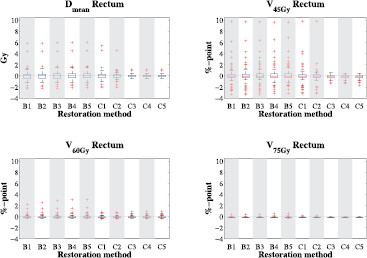
Figure 6. Boxplots showing differences of the restored minus the intended rectum dose parameters for all 80 scans for restoration methods B1–C5, based on the projected planning structures. Positive values point at higher values for the restored dose distribution. Each box plot indicates the median and the 25th and 75th percentiles of the obtained differences. The dashed lines depict the remaining differences which are not outliers. Values are defined outliers if they are more than 1.5 times the distance between the 25th and 75th quartiles away from the quartiles. The red marks indicate the outliers.
Download figure:
Standard image High-resolution image
Figure 7. Boxplots showing differences of the restored minus the intended bladder dose parameters for all 80 scans for restoration methods B1–C5, based on the projected planning structures. Positive values point at higher values for the restored dose distribution. Each box plot indicates the median and the 25th and 75th percentiles of the obtained differences. The dashed lines depict the remaining differences which are not outliers. Values are defined outliers if they are more than 1.5 times the distance between the 25th and 75th quartiles away from the quartiles. The red marks indicate the outliers.
Download figure:
Standard image High-resolution imageFigure 6 shows that even though defined as outliers, some of these difference values are still very low. When using method B5 only 8 scans show differences larger than or equal to +2 Gy for the Dmean and +2%-point for the V45 Gy, V60 Gy and V75 Gy. Using method C5 none of the scans obtain difference values larger than +2 Gy and +2%-point.
Figure 7 shows that on average the differences for all dosimetric parameters of the bladder are larger for the results of methods B. However, for both methods B and C the differences for the bladder are very small. Most scans differ less than +1 Gy for the Dmean and +1%-point for the V45 Gy and V65 Gy. The outliers reach maximum differences of approximately +1.6 Gy and +1.6%-point.
When comparing the results of methods B to the results of methods C, it can be seen that similar values are obtained. The largest differences are seen in the V45 Gy of the rectum, where for method B5 seven scans have a difference larger than +2%-point. Two of these scans also have a difference larger than 2 Gy for the Dmean. A scan of another patient has a difference larger than +2%-point for the V60 Gy of the rectum. For these 8 scans, the PTV overlaps with a gas pocket in the rectum of the repeat. Closer inspection revealed that the air cavity distorted the Bragg Peak resulting in less favorable rectum doses. To verify this assumption, we performed a full multi-criteria optimization using this repeat CT scan and the projected planning structures and compared the rectum dose values to the ones obtained from restoration. We found that in the fully optimized treatment plan the rectum Dmean was 28.1 Gy and the rectum V45 Gy 31.9%. The values obtained from the restoration were 28.1 Gy and 32.1% for respectively the Dmean and the V45 Gy. As the differences between these values are very small we conclude that our assumption is correct and the high dose values are indeed caused by a distorted Bragg Peak.
When using methods C, the rectum was restored better, but a larger part of the projected PTV received dose values higher than 107% of the prescribed dose (table 3). It should be noted that the dose of the distorted Bragg Peak was partly calculated inside the air cavity. Although this dose was contributing the rectum dose in the DVH calculation, in reality this dose will not be deposited in rectal tissue.
Results for actual repeat OAR structures of restoration methods B and C
The results in table 4 indicate that the target coverage can be effectively restored when evaluating on the actual repeat contours. Figure 8 shows the difference of the restored dose distributions for methods B5 and C5 minus the distorted dose distributions, i.e. without any restoration, for the actual repeat rectum (top) and bladder (bottom).

Figure 8. Boxplots showing differences of the restored minus the distorted dose parameters of the rectum (top) and bladder (bottom), for all 80 scans for restoration methods B5 and C5, based on the actual repeat structures. Positive values point at higher values for the restored dose distribution. Each box plot indicates the median and the 25th and 75th percentiles of the obtained differences. The dashed lines depict the remaining differences which are not outliers. Values are defined outliers if they are more than 1.5 times the distance between the 25th and 75th quartiles away from the quartiles. The red marks indicate the outliers.
Download figure:
Standard image High-resolution image
When looking at the results for the rectum (top figure 8) it can be seen that both methods B5 and C5 have median differences close to zero when comparing to the distorted dose distribution. In all plots it can be seen that the largest outliers have negative difference values, meaning that for those scans the restored dose distribution obtains lower dose values in the rectum than the distorted dose distribution. When looking at the V75 Gy after restoration, over 70% of the scans show differences equal to or smaller than zero. As can be seen in the boxplot, the remaining scans obtain very low difference values. For the Dmean, V60 Gy and V75 Gy all difference values remain below +4 Gy and +4%-point. For the V45 Gy there are 7 and 6 scans in respectively method B5 and C5 with a difference value larger than +4%-point.
For the bladder (bottom figure 8) we see that the differences between distorted and restored are very small for the V65 Gy. For the Dmean and V45 Gy the differences are larger, though over 92% of the scans obtain difference values below +4 Gy and +4%-point.
Though the dosimetric parameter values of the OARs can for some scans increase after restoration, this loss remains smaller than the gain that is found for the target structures (table 4).
Calculation times
The time needed for the energy adaptation, i.e. the restoration of the spot positions is independent of the restoration method and was on average 5.4 s (3.5–10.6). The re-optimization time includes the creation of the quadratic objective function, adapting the weight matrix and performing the minimization. Table 5 shows the re-optimization times for methods B1–B5 and C1–C5.
Table 5. Calculation times for the different B and C restoration methods. The mean is taken over all 80 scans.
| Weight re-optimization (seconds) | ||
|---|---|---|
| Mean | Range | |
| B1 | 0.7 | 0.4–1.7 |
| B2 | 1.5 | 0.9–3.6 |
| B3 | 2.2 | 1.3–4.5 |
| B4 | 3.1 | 1.8–5.9 |
| B5 | 3.8 | 2.2–7.7 |
| C1 | 0.9 | 0.4–2.5 |
| C2 | 1.8 | 0.9–4.0 |
| C3 | 2.7 | 1.3–5.6 |
| C4 | 3.7 | 1.6–7.5 |
| C5 | 4.5 | 2.3–9.0 |
The mentioned calculation times do not include loading of the CT scans, the original plans and the dose calculations. The most time-consuming and limiting operation was the calculation of the dose deposition matrix  (mean 4.3 min (range 2.4–9.6)), which occurs once between the spot restoration (i.e. energy adaptation) and the weight re-optimization. Optimization of the dose calculation speed was not part of this study.
Discussion
In this study several re-optimization methods were compared, all aimed at restoring the dose distribution that was distorted due to density changes. All restoration methods were designed for near real-time performance enabling online-adaptive proton therapy. The goal of the restoration was to get dose distributions as close as possible to the intended dose distributions in the structures used for treatment planning. We found that the restoration method that best restores the dose in the target structures is B5, which focuses on the target voxels. In every iteration, the target voxels that received either too much or too little dose were given a higher importance factor in the re-optimization. Using this method, all 80 scans had a restored dose distribution with a V95% ⩾ 98% and a V107% ⩽ 2% for the projected PTV structures used in the wishlist (table 1). When using method B5 the dosimetric parameters of the projected planning OARs showed on average very small differences from the intended values (⩽ +1 Gy and ⩽ +1%-point). Eight outliers were found with differences larger than +2 Gy and +2%-point. These outliers can all be explained by an air cavity partly overlapping the PTV. The air cavity negatively affected the shape of the Bragg peak (see figure 4), leading to a higher dose to the rectum after the restoration of the distorted dose distribution. For the worst outlier we generated a fully optimized treatment plan based on the repeat CT scan. The full optimization did not improve the dose to the rectum compared to the restoration, suggesting that the worsened rectum dose is due to the changed properties of the Bragg peak and that the restoration is close to the optimal result, i.e. a full re-optimization. An advantage of our method is that it can be applied using only the structures as contoured in the planning CT which means as soon as the daily CT scan has been aligned to the planning CT scan the restoration can start.
Besides method B5 method C5 also performed well. Although slightly better results for the target structures were obtained with methods B, methods C achieved lower dose values to the OARs. Using the methods C, the target coverage was slightly compromised, obtaining V95% values of less than 98% and V107% values of more than 2%. For example, for the projected PTV-low 67 scans had a V107% higher than 2% when using restoration method C5. However, the V107% was limited to 5.7%, which still may be considered clinically acceptable. As shown in table 5, the calculation time is similar for both methods. When comparing the use of 1 iteration with the use of more iterations, we found that the increased computation time using more iterations is negligible. However, using more iterations obtained fewer hotspots in the targets when using method B (as shown in table 3) and lower dose values to the OARs when using method C (figures 6 and 7).
In addition to the projected planning PTV and OAR structures, we also evaluated the restored dose distributions for the actual CTV and OAR structures in the repeat CT scans. We found that for the coverage of the CTV structures of the prostate, lymph nodes and seminal vesicles, the number of patients receiving acceptable V95% and V107% values for the targets, increased when applying a restoration method (table 4). Note that the intended treatment plan on the planning CT was optimized on a PTV volume, i.e. the actual target expanded by a margin, already anticipating some changes in shape and location. Performing a restoration on this PTV allowed for the CTVprostate to be sufficiently irradiated at every treatment day without having to include robustness in the optimization a priori. Similar as to the evaluation on the PTV, the best results were obtained when using method B5. For the OARs we compared the results of the distorted dose distribution, i.e. without restoration to the results of the dose distribution obtained with methods B5 and C5 (figure 8). We found that the volumes receiving a high dose were reduced a little, and only small differences were found in the mean dose of the organs. Overall we can conclude that performing the restoration has no negative effect on the dosimetric values of the OARs.
Taken together, our findings prove the principle that clinically acceptable restorations for density changes can be obtained for prostate cancer patients within 10 s, when excluding the calculation of the dose deposition matrices. The calculation of these matrices currently takes several minutes. We believe that with some improvements of the dose engine this calculation time can be significantly reduced.
Though many more re-optimization methods are possible, as well as methods of updating the weight matrix  (see equation (1)) between iterations, only four main methods (A–D) were considered during this investigation. Method A was selected to see the effect of minimal effort; by not using any importance factors, the method is very general and very fast. Methods B and C, in which we focus on the targets and OARs, were selected on the basic principle that in treatment planning the goal is always to get a high dose in the targets and a low dose in the OARs. Method D, in which higher importance factors are given to structures with higher differences, was inspired by our re-optimization method which aims to minimize the differences between the intended and the achieved dose.
In this study we analyzed the mean dose to OAR. To test whether the method also works for more serially responding organs, we applied a maximum dose objective to the rectum in the generation of the intended treatment plan. The results of applying restoration methods A, B5, C5 and D5 on these cases were similar to the results of the previously discussed prostate cancer cases. Methods A and D yielded coldspots and hotspots, while methods B5 and C5 obtained acceptable results. Other approaches have not been investigated, as clinically sufficient results were already obtained using the methods developed and evaluated in this study. However, it is possible that for other treatment sites other restoration methods are more suitable.
Looking at the results of the restorations the difficulty seems to be in the restoration of the PTV-low as projected on the repeat CT scan. A possible explanation is that less degrees of freedom are available for the optimizer to restore the dose distribution as the dose to each lymph node is mostly delivered by one of the beams.
The developed restoration method aims to return to a clinically acceptable treatment plan which has already been through some level of quality assurance (QA). One could therefore assume that returning to this plan yields acceptable results. Some level of QA is however still required, as errors are always possible. This should involve a check on indicators that identify successful restorations. These indicators are for example PTV coverage and the difference between the intended and restored dose distribution e.g. using gamma evaluation if gamma analysis can be performed sufficiently fast. Also flagging large changes in spot weights and WEPL corrections will be important as indicator of unsuccessful restorations. Furthermore, online QA of dose delivery errors is also required, as pre-treatment patient-specific QA cannot be performed in the online-adaptive setting. This is being developed in a project closely linked to this work, which aims at developing proton range verification for online QA using prompt-gamma imaging.
In generating the intended treatment plans, CTV-to-PTV margins were used to adapt for inter- and intra-fraction motion of the structures. With these margins, the developed dose restoration method based on the projected contours has shown to obtain clinically acceptable restorations for prostate cancer patients. Evaluating on the actual contours obtained sufficient CTV coverage for most CT scans (table 4) and acceptable values for the OARs (figure 8). The intended treatment plans were generated using normal margins and no additional robustness settings. This shows that the re-optimization method can quickly adapt for changes, even if the treatment plan is not robust. If greater daily shape changes are expected, for instance in cervical cancer, the method will still work, but the PTV or internal target volume becomes very large. Therefore the aim will then be to first reduce the PTV, which can be achieved by implementing a plan-of-the-day approach based on a pretreatment established library-of-plans. After selecting the most tight fitting plan, our dose restoration method can be used to correct for density changes. We believe that will also work for other tumors in the pelvic region such as bladder cancer. To determine with how much the PTV can be reduced and whether this works for tumor sites outside the pelvic region needs further research.
In prostate cancer inter-fraction and intra-fraction variations in position and shape of the target volume and density changes along the proton beam paths can contribute to loss of coverage. Various studies have shown that the contribution of intra-fraction motion is much less than inter-fraction motion if treatment times are kept sufficiently short. The speed of the dose restoration is therefore of great importance. Residual shape changes of the target volume caused by intra-fraction motion can be accounted for by adding a small extra margin. If robustness is included in the initial plan we expect that due to the restoration of the spot positions the robustness will to some extent be preserved. The re-optimization of the spot weighs however might reduce the amount of preserved robustness. To what extent the robustness will be preserved and whether it is necessary to include robustness to tackle intra-fraction density changes requires further investigation.
The treatment plans generated in this study used two laterally opposing beams traversing through the hip bones. Rotational variation of the hip bone gives rise to density variations along the pencil beam paths. On top of this, for the aligned scans shifts of the lymph nodes in the direction of the beam of at most 5 mm were detected, as well as anatomical changes of the seminal vesicles and prostate below 5 mm and 3 mm respectively. The small changes in the anatomy of the prostate itself can be explained by the scan alignment on the intra-prostatic markers. Andersen et al (2015) investigated plan robustness for different beam angles for prostate cancer patients. In their study they found that for the lymph nodes a low WEPL variation was found for beam angles around 40° and around 150°–160° for the left and corresponding angles for the right lymph nodes. Our method starts by correcting the WEPL, obtaining clinically acceptable restorations for all target structures. As the detected movement of the lymph nodes has the same dosimetric effect as movement of the hip bones, we can assume that the method will also successfully adapt for the changing positions of the hip bones.
Zhang et al (2011) described a dose-adaptation method using only an energy adaptation. For the original DET treatment plan the adaptation obtained restorations which, when averaged over five shift datasets, differed less than 1% for the prostate D98%, D50% and D2%. For the IMPT plan the restorations did not show sufficient improvements. These results were obtained with a phantom prostate patient in which only the prostate and femoral heads were delineated. In our study we used real patient CT scans and the rectum and bladder were used for evaluation. For all patients the targets V95% and V107% were restored to clinically acceptable values. Zhang et al (2011) did not report on hotspots in the restored dose distributions. In the present study the restored dose distributions with respect to hotspots were evaluated visually. Though the restored dose distributions were less homogeneous than the planned distributions, no clinically significant hotspots were observed. This, however, does not guarantee they will never occur. Our restoration method could be improved by including a quality-check and intervention system to prevent adverse effects on the dose distribution.
Bert et al (2007) created a method that adapts the pencil beam positions as well as the beam energy (WEPL) during the treatment. To our knowledge they however did not change the pencil beam weights.
The difference between the method of Bert et al and the method described in this work is in the steps that the methods use. Bert et al adapt the pencil beam positions and the beam energies, while this method adapts the beam energies and the beam weights. The difference between the two methods can be explained by the difference in application; Bert et al compensate for intra-fraction target motion while we compensate for inter-fraction density changes.
For fractionated treatments it can be assumed that the impact of density changes are to some extent averaged out. However, this cannot be guaranteed for hypo-fractionated treatments. This method may therefore help to safely implement hypo-fractionated IMPT treatments by reducing the impact of the density changes before each treatment fraction. Another advantage of this restoration method is that it can replace the use of a rectal balloon. These balloons are sometimes inserted in prostate cancer patients in order to reduce the density changes and prevent large air cavities. These balloons however have to be inserted at every treatment day and can be a discomfort to the patients. In some cases the balloons are not even tolerated (Ronson et al 2006). In this light our proposed restoration method may be an attractive alternative.
Conclusions
The impact of density variations on the pencil beam path in IMPT can be reduced by performing an automated dose restoration procedure consisting of a WEPL correction of the pencil beams, followed by a re-optimization of the pencil beam weights. Only performing the WEPL correction does not yield clinically acceptable results. The fast performance of the restoration method paves the way to future near-real time online-adaptive proton therapy.
Acknowledgments and conflicts of interests
The CT-data with contours were collected at Haukeland University Hospital, Bergen, Norway and were provided to us by responsible oncologist Svein Inge Helle and physicist Liv Bolstad Hysing.
This study was financially supported by ZonMw, the Netherlands Organization for Health Research and Development, grant number 104003012 and by Varian Medical Systems. Erasmus MC Cancer Institute also has research collaborations with Elekta AB, Stockholm, Sweden and Accuray Inc, Sunnyvale, USA.