
Abstract
With a complex topic such as aerodynamics, subtle points are critical. In this work images illustrating air flow around wings and aerofoils were studied to explore misunderstandings in aerodynamics education. While these images are common in textbooks and popular science media, this study was limited to the 135 physics education articles on the topic of lift, of which 49 contained illustrations of air flow around an aerofoil or wing. These 49 cases were included for qualitative comparison using visual semiotics. It was found that 28% of images did not include upwash, and only 44% included stagnation points. For the case of 2D flow around aerofoils 30% were illustrated correctly, while for wings 75% were correct. These results excluded the seven completely incorrect illustrations where common misconceptions were presented as facts. Most illustrations of flow around an aerofoil incorrectly depicted flow around a wing.
Export citation and abstract BibTeX RIS

Original content from this work may be used under the terms of the Creative Commons Attribution 4.0 license. Any further distribution of this work must maintain attribution to the author(s) and the title of the work, journal citation and DOI.
1. Introduction
There is a misconception that the aerodynamics of fixed wing flight is simple. Prescod-Weinstein (2022) recently expressed this well on the topic of 'why planes fly', referring to Shotwell's 'implicit understanding'. The concept has been discussed in the literature previously, and is about the difficulty in ascribing cause and effect to the field solutions of an elliptic partial differential equation (Auerbach 1988). In the best case we can refer to a simplification (Babinsky 2003), while attempts from first principles are wrong (Linton 2007, Robertson 2014). An actual understanding of why the aerodynamic force of lift is produced, requires some understanding of Navier–Stokes (Wild 2021).
Maxwell's equations are commonly covered in first year physics, at different levels. At the lowest level, the meaning of each equation can be discussed, and they are typically used separately to solve some quantitative problems. Combining them to give a wave equation might also be demonstrated. The Navier–Stokes equations are only slightly more complicated and have been featured on the YouTube channel Numberphile (www.youtube.com/watch?v=ERBVFcutl3M). The solutions from Maxwell's equations that describe electric and magnetic potentials are analogous to simple potential flows originally used in fluids; in fact, as a mathematician, Maxwell used the theory from fluids to formulise Faraday's practical work (Joseph 2022). Navier–Stokes adds the extra term viscosity to these early abstract mathematical fluids, which helps them capture many practical features of real fluids, including lift (Barnes and Potter 1974). While Navier–Stokes is not covered in many physics texts, it is covered by Feynman (1964), and there have been previous attempts to make them more available (Schneiderbauer and Krieger 2014).
Bungum (2013) studied images in upper secondary school physics textbooks as a means of visual communication. They noted conventional images that make use of symbols are intended to help the reader form an understanding. Three elements are discussed from Dimopoulos et al (2003), classification, framing, and formality. For this work, classification and formality are of interest. Zetie (2003) previously reported a common visual misconception for air flow around a wing, the classic flat bottom flow (see figure 1), which has been in use for decades (Pope and Otis 1941). In contrast, correct images were used in the '1941 edition of the Civil pilot training manual' (Webster 1947). The aim of this paper is to review all the image presented in the education literature to explore misunderstandings in aerodynamics education, and by understanding the aspects of flow visualisations, to identify what feature are needed for an ideal image that conveys the correct concepts.
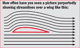
Figure 1. Incorrect visualisation of streamlines around an aerofoil showing flat bottom flow (Zetie 2003).
Download figure:
Standard image High-resolution image2. Background
There are complications associated with visualising the flows around aerofoils and wings. While real flow visualisations have inherent value, the scale of the flow features is orders of magnitude greater than the scale of the aerofoil. For example, if this printed page (landscape) was the domain of interest, a modern simulation would only be of an aerofoil 6 mm long and 0.5 mm wide; '——' is approximately 6 mm long. Another intrinsic complexity is that flow is typically visualised in a steady state, such that it does not change over time. However, important features are transient, and hence cannot be captured directly with an image. The intrinsic complexities are further exacerbated by extrinsic complexities. These include any underlying conceptual misunderstandings. This is illustrated by Zetie (2003) where people visualise what they think intuitively should happen, or what conforms to the simplified model they believe is correct.
The key element of flow visualisation is the streamline, a significant classification element (Dimopoulos et al 2003), or content specialisation as referred to by Bungum (2013). As such, the meaning and significance of the streamline needs to be understood. Streamlines represent the velocity vector field that is the solution to the Navier–Stokes equations. If a massless 'test particle' is dropped into a flow, it will travel along a streamline. Think of how a test charge moves relative to electric field lines. As such, the streamlines will capture information about the displacement, velocity, and acceleration of the flow.
To be able to evaluate flow visualisations, the correct flow needs to be understood. A full qualitative justification for the correct flow is given in the

Figure 2. Options for stagnating streamlines, (a) the flow splits at the leading edge, (b) the flow splits somewhere in front of the aerofoil, or (c) the flow needs to split below the aerofoil.
Download figure:
Standard image High-resolution imageReferring to figure 2, the points of interest, literally the red dots, are referred to as stagnation points. These are locations where the fluid velocity is zero; that is, the flow has stagnated. According to Bernoulli's principle, these correspond to locations of maximum static pressure. In an aviation context, we note the dynamic pressure has been converted to static pressure, maintaining the total pressure (the constant of the streamline from Bernoulli).
These two defining features become important when looking at flow visualisations in the literature. Consider the illustration from Robertson (2014), reproduced in figure 3. Here both the flow ahead of and behind the aerofoil are incorrect. The intuition about the leading edge being responsible for the flow splitting is shown, and the continuation of the flow down at the angle of attack (a), is illustrated. This is because the underlying principle presented by Robertson (2014) is a statement of Newton's 3rd Law to explain lift, which implies such a flow field.

Figure 3. Incorrect streamlines around an aerofoil (Robertson 2014).
Download figure:
Standard image High-resolution imageAnother common type of flow that can be visualised is what Hewitt (2004) calls 'billiard-ball' physics. In his approach to conceptualise all introductory physics, Hewitt noted that the model of molecules and how they behave in terms of pressure as billiard-balls bouncing around could not explain the flow around a wing or a fan. Some refer to this as the 'hail of bullets' model, and Newton himself derived his famously flawed sin squared law. This is illustrated in figure 4. The arrows describing the trajectories of the molecules are reflected from the plate, and hence the reason a sin squared law results for the lift force. Similarly, the geometry from figure 3 results in a sin law for the lift force. However, the relationship between the angle of the plate, called the angle of attack, and the lift force is linear. For complex high lift configurations, this linear relationship between lift and angle of attack can extend to 45 degrees (Smith 1975).
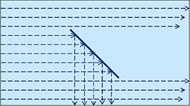
Figure 4. Billiard-ball physics applied to explain lift, called the ski effect, or hail of bullets model.
Download figure:
Standard image High-resolution image3. Methodology
A detailed search of the literature was conducted, through Google Scholar, Scopus, JSTOR, and publishers' databases (Science direct, Taylor and Francis, etc.). In Google Scholar, the 'Cited by' link for every collected paper was searched, as was its reference list. This provided confidence that the population of physics education literature on lift and flight mechanics is limited to the 135 articles found, up to and including 2021. Of these, only 49 included one or more images of streamlines (air flow) around an aerofoil or wing. The streamline diagrams was the data for the qualitative research utilising a visual methodology (Banks 2007), specifically the study of images and what they mean (Van Leeuwen 2004). The image analysis utilised a deductive coding approach, where a start list of proposed codes was informed by the previously discussed aerodynamics. Additions to the coding structure were made as novel features were identified. An open coding approach was implemented, where literally every line (streamline) was coded in terms of notable features (direction, upwash, downwash, stagnation, etc). These features literally align with those of Allen (1998), 'space and event, force and resistance, density, distribution and direction'. The open coding was essential to minimise subjectivity (Leedy and Ormrod 2013). The data is neither constrained to the positivist nature of the images, nor interpretivism; rather, technical details within the images and their implications in terms of aerodynamics is the data. That is, the data represent the narrative of the image, which is 'the intentional organization of information apparently presented within (...) an image' (Banks 2007).
4. Results and discussion
The resultant coding structure was:
- 1.Essential features
- a.Upper (Up) = flow over the upper surface
- b.Lower (Lo) = flow under the lower surface
- c.Stagnation (Stag) = stagnation point(s)
- d.Upwash (UW) = flow raising ahead
- e.Downwash (DW) = flow behind displaced, deflected, or directed down
- f.Aerofoil = object identified as an aerofoil (2D flow applies)
- g.Wing = object identified as a wing (3D flow applies)
- h.W = rear far field vertical velocity
- i.2D = NAND (1.f, 1.h) × 1.f
- ii.3D = AND (1.g, 1.h) × 1.g
- 2.Secondary features
- a.Pressure (P) = information about pressure distribution
- b.Trailing edge vortex (TE V) = transient starting vortex
- c.Tip vortices (Tip V) = wing tip vortices
- d.Circulation (Cir) = concept of circulation
- 3.Associated flow
- a.Cylinder (Cyl) = flow around a simple cylinder
- b.Magnus (Mag) = flow around a rotating cylinder or sphere
- c.Potential flow (PF) = flow around an aerofoil without viscosity (circulation)
- 4.Misconception
- a.Inverted (In) = showing the streamlines for an inverted wing/aerofoil
- b.Flat = image of flat bottom streamline
- c.Ski = bullet or billiard-ball like molecules impacting and deflecting
- 5.Problem = misconception presented as fact or other serious issue
Each of the above items (except for 5) was coded with a binary value. From these, combinations were possible; specifically, a derived property of the flow correctness was created (1.h, i and ii) combining the structure (aerofoil or wing) and the far field velocity W. If W = 0 for an aerofoil, a code '2D' was 1, and for W = 1 for a wing, then the code '3D' was 1. That is, the flow correctness was true. The sum of 1.a to 1.e plus 1.f or 1.g and i or ii gave a score, out of seven.
Table 1 shows the essential features, with flow over the upper surface the most common feature. Less than half include a stagnation point, and only three quarters illustrate upwash; it should be noted that some cases without stagnation points have minimal upwash, suggesting a stagnating streamline is key to correctly illustrating upwash. Given only 16 cases are identified as flow corresponding to wings, there are too many (30) with a vertical velocity component in the far field. Only 8 of the 27 aerofoil images (less than one third) have correctly illustrated 2D flow. For wings, this increases to almost three quarters. Only 8 of 42 cases had illustrations which included all the essential features, for either a wing or aerofoil with correct flow. That is, only 19% of cases had a score of seven out of seven. Of those, six were for 2D flow and two were for 3D flow. Of the 12 3D flow visualisations, only two included stagnation points.
Table 1. Counts for essential features of the flow visualisation (maximum possible score 42).
| Up | Lo | Stag | UW | DW | Aerofoil | Wing | W | 2D | 3D |
|---|---|---|---|---|---|---|---|---|---|
| 41 | 40 | 19 | 31 | 40 | 27 | 16 | 30 | 8 | 12 |
In table 2, results show that just over a quarter of cases illustrated the common incorrect flow with a flat bottom streamline. Around 7% showed inverted aerofoils/wings with correct streamlines around them, and 5% illustrated the ski/bullet/billiard-ball misconception. In general, authors appear to not illustrate incorrect flow. Given that lift is experimentally measured with pressure, only 12% of cases included pressure information. The pressure distribution and circulation only appeared in a single case together, tending to be mutually exclusive when present, although they are intimately connected (Wild 1966). Only four of the six tip vortices were associated with illustrations that referenced wings, noting they are not a feature of aerofoils. Four of the circulation cases were also Magnus cases, and although the resultant flow field is similar, an aerofoil is not rotating so the discussion is superfluous. Similarly, all but one of the potential flow cases coincided with circulation, which are commonly associated (Wild 2021).
Table 2. Counts for secondary features, associated flows, and misconceptions addressed.
| Secondary | Associated | Misconceptions | |||||||
|---|---|---|---|---|---|---|---|---|---|
| P | TE V | Tip V | Cir | Cyl | Mag | PF | In | Flat | Ski |
| 6 | 3 | 6 | 6 | 6 | 6 | 5 | 3 | 11 | 2 |
Figure 5 presents all the features that may be illustrated in the flow around an aerofoil. Points 1–5 address codes 1.a to 1.e, consecutively. The rear far field flow should also be correctly illustrated (7). The concept of angle of attack is also very easy to include (8), given the incoming freestream flow (11) is horizontal. Basic pressure information, especially around the stagnation points can also be illustrated (9), with the potential for more isobars. The minimal pressure information illustrated around the front stagnation point highlights some important features; first, along the stagnating streamline there is an increase in pressure to the stagnation point, and then the resultant pressure gradient force (PGF) across the flow is greater in the upwards direction resulting in greater acceleration, relative to the downward direction. Finally, the difference in velocity can be illustrated (10) which relates to circulation.
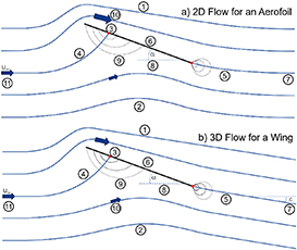
Figure 5. Feature of ideal flow illustrations, (a) for an aerofoil in 2D and (b) for a wing in 3D.
Download figure:
Standard image High-resolution imageGiven aerodynamics is dynamic, the illustration in figure 5 is only a representation of real flow, to convey key features. Importantly, where local pressures are greater and less than the freestream pressure depends on the angle of attack, with stall being the classic example. For a wing, the rear far field flow (7) can highlight the downwash angle epsilon, ε (this is not equal to α, and reduces as speed increases). The contentious issue with figure 5 is likely the use of a flat plate (6) and not a modern low speed aerofoil like a NASA-LS(1)-0417 which is very efficient, very curved, and very thick (relatively speaking). The flat plate is an essential tool, as it removes the misconception that the curved shape is responsible for the flow and hence lift (Wild and Wild 2023), a common misconception. The other advantage of the flat plate is that it forces the front stagnation point to be on the underside as it can only be at the LE when the angle of attack is zero.
5. Conclusion
Ultimately, aerodynamics is complicated. This is because it is underpinned by a set of equations even more complex than Maxwell's, those of Navier and Stokes. While not covered in first year physics, aerodynamics is not possible to understand without them. While many recent efforts have incorrectly used Coanda to explain lift, all the features they strive to explain are covered by the inclusion of viscosity, as done by Navier and Stokes. To abstract the knowledge, flow visualisation using streamlines are a common tool that make use of content specialisation, with a high degree of image formality. When intuition is used to illustrate the invisible flow of air around an aerofoil, misconceptions are inevitable. Key elements of correct flows were presented, as were common misconceptions. The key difference between 2D and 3D air flow around aerofoils or wings was also discussed; that is what happens to the flow in the rear far field. For 2D flow, the streamlines return to the horizontal. For 3D flow, the streamlines remain angled below the horizontal, with the downwash inducing a downwards velocity component. Using a visual (semiotic) methodology, the flow illustrations of 49 education papers on lift were analysed. Open coding identified all the unique features. Seven of the cases used wholly incorrect flow illustrations, embodying common misconceptions of aerodynamics. Most cases (27) presented flow around aerofoils, and very few presented the flow correctly in the rear far field (8). Only 19% of cases illustrated all primary features of the flow, with stagnation points most often omitted, which also makes upwash harder to convey. A proposed ideal figure was presented, depicting 11 features of the flow, noting key differences for 2D and 3D flow.
Dedication
My study of lift education in 2022 included my 15 year-old son, Graham Derrick Wild. I helped him build a wind tunnel for his high school science project, and he used it to win first place (engineering) in the state science fair (SEAACT Science and Engineering Fair), something I never did. Sadly, he passed away on the 14th of December, 2022, not long after that achievement, and before learning that he had become a published author (Wild and Wild 2023), something he was looking forward to. I miss his collaboration and contribution.
Data availability statement
All data that support the findings of this study are included within the article (and any supplementary files).
: Appendix
It is becoming more and more common to see explanations of lift which are just statements of Newton's 3rd Law, action/reaction; that is, lift is the reaction to air deflected downwards by a wing. Experimental aerodynamicists measure the pressure distribution around an aerofoil, and hence, a pressure difference statement can explain 'how' a wing produces lift. Also, computational aerodynamicists use circulation to calculate lift, and hence a circulation statement can explain 'how' a wing produces lift. Importantly, 'why' a wing produces lift is explained by Navier–Stokes. In simple terms (Mclean 2012), a body in a flow is an obstacle and produces a PGF, and although a mathematically ideal fluid (potential flow) will give symmetric flow, viscous effects result in flow asymmetries. The important result is the rear stagnation point moves to the trailing edge. That is, the Kutta condition arises due to viscous effects (Liu et al 2017, Liu 2021). It should be noted that most label the viscous effect as the Coanda effect, and this is incorrect (Mclean 2012), even though some continue to suggest Coanda is involved in lift (OSS 2022). The Coanda effect is real, and arises due to viscosity, but applies to jets of fluid which are not present around a simple aerofoil. That said, high lift devices can make use of the Coanda effect, such as the blow flaps of the Blackburn Buccaneer and the Lockheed F-104 Starfighter (Beck et al 2015).
Mclean (2018) inaccurately states 'most wings are of high enough aspect ratio that the flow in cross sections is qualitatively the same as if the span were infinite, and the flow were two dimensional.' It is crucial that the difference between 2D and 3D flow is understood. This distinction is made in the way aerodynamics is taught to engineering students, first 2D then 3D (Anderson 2016). While the two flows possess some similarities, they have critical differences.
The essence of 3D flow around a wing with a finite span is enshrined in the aviation safety regulations for aircraft separation (Gerz et al 2002). This is because aircraft generate wing tip vortices, which are a serious hazard to aircraft behind. Vortices result because flow above and below the wing are not independent due to the wing tip. That is, the flow from the relatively higher pressure underneath the wing tends to flow towards the wing tip, while above it tends to flow towards the wing root; the flow around the tip couples with the freestream flow resulting in a vortex (Anderson 2005, Somerville et al 2016). In a 2D case, spanwise motion of the flow is not possible. That is, in a wind tunnel test wing will have a wingspan equal to the width of the tunnel test section (referred to as an infinite wing), as shown in figure 6. Hence, the flow pattern of both 2D and 3D wings needs to be considered.

Figure 6. An aerofoil in the Langley 2D low-turbulence wind tunnel, spanning the width of the test Section (Von Doenhoff and Abbott 1947). This work is in the public domain.
Download figure:
Standard image High-resolution imageWhen comparing 2D or 3D flow for lift, a critical difference is in the flow behind that aerofoil or wing. The flow behind the wing exhibits downward turning, referred to as downwash in aerodynamics; however, the term downwash is typically exclusively used for 3D flow. An absence of downwash is typically associated with an incorrect understanding of lift corresponding to the potential flow solutions that resulted in d'Alembert's paradox (Wild 2021). The exact nature of the downwash is the difference between 2D and 3D flow and appears to be an ill-considered aspect in flow illustration. This is surprising given the key diagram for this has been seen by countless practical aviators who likely have not appreciated the subtlety. This key diagram is figure 1.30 from Hurt (1965), reproduced in figure 7. Hurt illustrates the vertical velocity component of the air flow labelled as W, for both 2D and 3D. For 2D flow with only the 'bound vortex', W is zero in the far field at the rear of the aerofoil. For 3D flow with 'coupled bound and tip vortices', W in the far field is twice the value at the aerodynamic centre, downward. The 'coupled bound and tip vortices' result in a flow that continues to move downward at a constant velocity even well after the aircraft has passed, and hence the previous statement about regulation on the separation of aircraft. Importantly, for a 2D wing the vertical velocity of the flow returns to zero; hence, how 'downwash' manifests in 2D flow is not intuitive. Mclean (2012) explains that while even though the local vertical velocity tends to zero, there is a distribution of the vertical velocity components. Importantly, the end result of the momentum transfer is to transmit the force from the wing to the earth's surface (Prandtl 1921, Mclean 2012). It should be noted there are those that incorrectly believe this is not the case (Anderson and Eberhardt 2009).

Figure 7. Wing vortex system (Hurt 1965), illustrating the vertical velocities in the vicinity of the wing. This work is in the public domain.
Download figure:
Standard image High-resolution image
For 2D flow streamlines must return to the horizontal, as they were prior to the upwash, while for 3D flow, streamlines must be directed downwards at the downwash angle (epsilon), creating induced drag (Anderson 2016). Although, it should be noted that there is no action at a distance, and the fluid acts on the wing at the surface via pressure, with viscosity producing the flow asymmetry. As such, relying solely on a momentum transfer statement ignores much of the fluid mechanics. This is not paradoxical, rather the complexity is explained by Mclean (2012) in terms of where the surfaces of the control volume (CV) of interest are placed. Referring to figure 7, there are two configurations of interest, both using the earth's surface and the top of the atmosphere, as the lower and upper surfaces, respectively. The first has the inlet immediately ahead of the wing (point 2) and the outlet is immediately behind the wing (point 3). The result here is maximum positive vertical momentum into the CV and maximum negative vertical momentum out (the dashed line), resulting in a significant change in momentum across the aerofoil. The second has the inlet and outlet very far away, ahead and behind, respectively (points 1 and 4). This results in no vertical momentum in or out (the dashed line has returned to the horizontal centreline). Instead, all the force is the over pressure at the earth's surface, as shown by (Prandtl 1921). This second example is analogous to the method used to measure lift for NACA aerofoils by NASA (Von Doenhoff and Abbott 1947).
Supplementary data (<0.1 MB PDF)