

Abstract
According to the classical Eshelby inclusion problem, we introduce a new linear relation to calculate internal stresses in γ/γ' microstructures of superalloys via an effective stiffness method. To accomplish this, we identify regions with almost uniform deformation behavior within the microstructure. Assigning different eigenstrains to these regions results in a characteristic internal stress state. The linear relation between eigenstrains and internal stresses, as proposed by Eshelby for simpler geometries, is shown to be a valid approximation to the solution for complex microstructures. The fast Fourier transformation method is chosen as a very efficient numerical solver to determine the effective stiffness matrix. Numerical validation shows that this generalized method with the effective stiffness matrix is efficient to obtain appropriate internal stresses and that it can be used to consider the influence of internal stresses on plasticity and creep kinetics in superalloys.
Export citation and abstract BibTeX RIS
1. Introduction
Ni-base and Co-base superalloys are known for their outstanding creep resistance at high temperatures. The creep behavior and corresponding mechanisms related to the dislocation motion in the microstructure of these alloys have been well investigated experimentally by different research groups, such as the general introduction of creep and dislocation structures in some typical superalloys [1–3], the formation of dislocation networks on γ/γ' interfaces at high temperatures [4], the orientation dependence of creep under different loading conditions [5, 6], as well as the shearing of  precipitates with stacking faults [7]. In addition, through comprehensive dislocation dynamics modeling, the important creep mechanisms were clarified and validated [8]. Since the creep behavior is attributed to the particular microstructure where softer face centered cubic γ matrix is strengthened by stronger cuboidal or spherical L12-ordered
  precipitates [9], the crystal plasticity modeling of creep deformation should be also based on this microstructure. Due to the γ/γ' lattice mismatch and the inhomogeneous deformation in γ matrix and
  precipitate during creep, internal stresses are generated, which influences further deformation and rafting of precipitates [10–14]. Although several dislocation-based constitutive models have taken the importance of internal stresses into account [15–17], their calculations mainly depend on the common microstructure with narrow γ channels and cubic
  precipitate. To overcome this restriction, a new method is developed here to calculate internal stresses in γ/γ' microstructure of superalloys numerically, by generalization of Eshelby inclusion problem [18, 19] and identification of regions with uniform deformation behavior. This method can be used not only for cubic
  precipitates, but also for different morphologies, such as spherical
  precipitates. It is worthy to note that the calculated internal stresses in the present work result from the eigenstrains in different regions which are sum of the accumulated plastic strains and misfit strains at a certain time, where the microstructure and the deformation state are known. During the deformation, the internal stresses can be updated by using this method in every time step. This method can be easily implemented in crystal plasticity finite element (FE) models to consider the evolution of internal stresses while simulating creep or plastic deformation of larger structures or components. In our work we only solve the linear elastic problem relating the eigenstrains to internal stresses, but we note for the sake of completeness that recent developments on spectral solvers also allow them to be used for finite deformations and nonlinear materials [20–22].
2. Determination of the effective stiffness matrix
Under external load the lattice mismatch in superalloys leads to the inhomogeneous deformation in different channels [13]. The internal stresses caused by the misfit strain and the deformation heterogeneity play an important role on the deformation. If the elastic and plastic strains are known, the total stress  including the external stress
  and the internal stress
  are given as

where  is the elastic stiffness matrix,
  is the elastic strain,
  is the plastic strain,
  is the misfit strain, and
  is an assumed effective stiffness matrix connecting the internal stress with plastic strain and misfit strain. In this paper, we aim to determine
  , so as to calculate the internal stress through it.
In view of the characteristic γ/γ' microstructure of superalloy single crystals, a cubic representative volume element (RVE), similar to that used in [13, 23, 24], containing one cubic  precipitate surrounded by narrow γ matrix channels, is utilized to determine internal stresses. With known eigenstrains in the RVE with periodic boundary conditions, the internal stresses can be calculated by the fast Fourier transformation (FFT) method [13, 25–27]. The RVE is treated as a material with a reference stiffness
  , which is a volume average of local elastic stiffnesses. Analogous to the solution of the Eshelby inclusion problem [18, 19], by assigning the eigenstrain
  to the local strain, the internal stress on each FFT grid can be obtained by

where the mean internal stress  is the volume average of
  . The local internal stress fluctuation
  is identical to the constraint stress caused by the corresponding strain fluctuation
  :
:

where  is the Eshelby tensor and
  is the unit tensor. We extend equation (3) to consider the interaction among FFT grids

where  is the displacement to produce
  . We use the same Fourier transformation method shown in [13] to solve equation (4), and finally to gain the internal stress.
Based on this FFT method and assuming the deformation of the RVE follows a simple constitutive equation as

where  is the strain rate, A is the reference parameter and n is the stress exponent, the full fields of plastic strain and internal stress in the RVE can be calculated. Before the deformation starts, the misfit strain determines the internal stress. Here, in
  precipitate
  and in γ channels
  , where δ is the lattice mismatch ratio. As the plastic strain is generated, we combine the misfit strain and the plastic strain as the general eigenstrain to determine the internal stress in each time step. The new internal stress influences the plastic strain in the next time step. From an example for a RVE with approx. 66% volume fraction of a cube
  precipitate in figure 1, we can see that the plastic strains and the internal stresses in some regions are similar under a constant uniaxial tensile load of 300 MPa along [001] direction. Meanwhile, the internal stress varies with the plastic strain gradually during the deformation. Furthermore, the regions with similar plastic strains are also found in figure 2 for other two loading directions. These results depend on the model parameters in table 1 and the elastic constants at room temperature of a Ni-base single crystal superalloy [28]. Since the
  phase is stronger than γ phase, we use a smaller A for
  phase.

Figure 1. The evolution of full fields of equivalent plastic strains (a) and equivalent von Mises internal stresses (b) in the RVE with a cubic  precipitate during the deformation under a constant uniaxial tensile load of 300 MPa along [001] direction.
Download figure:
Standard image High-resolution image
Figure 2. Full fields of equivalent plastic strains in 500 time steps in the RVE with a cubic  precipitate under a constant uniaxial tensile load of 300 MPa along [110] direction (a) and [111] direction (b).
Download figure:
Standard image High-resolution imageTable 1. Model parameters.
| n | 3 |
|---|---|
| A in γ (MPa−n) |

|
A in  (MPa−n) (MPa−n) |

|
| δ | −0.0015 |
If this RVE is only considered as an integration point in a FE method, the detailed plastic strains and internal stresses on each FFT node are not required, and it is sufficient to know the solution in the regions of homogeneous deformation behavior. According to the observation and the analysis of plastic strains in the RVE, as well as the approach proposed by Fedelich [16], the plastic deformation can be taken approximately uniform in each channel and in the  precipitate. Therefore, the RVE generally consists of four main regions which are one
  phase and three γ channels in three given orthogonal directions of cartesian coordinate system, respectively. Based on equation (8) in the literature [16], the uniform plastic strain and the misfit strain in these four regions can be expressed as
where  ,
,  ,
,  , and
, and  are deemed as eigenstrains for the calculation of internal stresses.
As shown in figure 3, when  ,
,  ,
,  , and
, and  are assigned to the corresponding FFT grids in x-, y-, z-channels and precipitate, respectively, and the FFT grids in the edge and corner areas take the average values of eigenstrains in adjacent channels, the full field of internal stresses in the RVE can be obtained by the introduced FFT method as well. By averaging the values in the respective regions, the
  ,
,  ,
,  , and
, and  are adopted to represent the internal stresses there. For a large precipitate and narrow channels, the areas in the edge and corner can be neglected. The general subdivision of the RVE is displayed in figure 4.
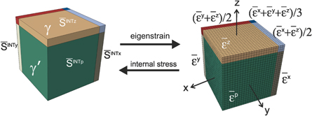
Figure 3. Schematic diagram of one eighth of the periodic RVE, indicating the subdivision into regions with uniform deformation behavior. The eigenstrains in these regions are correlated to internal stresses via the FFT method with a regular grid. The different colors represent different regions.
Download figure:
Standard image High-resolution image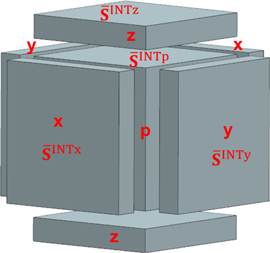
Figure 4. Schematic diagram of subdivision of RVE with a cubic  precipitate.
Download figure:
Standard image High-resolution imageEven though the FFT method is an efficient way to calculate internal stresses, it is still time-consuming for long-time deformation of a large component with lots of material points. We introduce a mathematical linear relation between internal stresses and eigenstrains with an effective stiffness matrix as

Extending  and
and  to four sections respectively, equation (7) becomes
Taking six components of each stress (strain) tensor into account, there are 24 independent stress (strain) components totally. Hence, the entire effective stiffness  should be a 24 × 24 matrix. In order to determine the effective stiffness matrix, we assign the value of '1' to each of strain component (e.g.,
  ,
,  ,
,  , ...), keeping other strain components to '0'. By means of the method mentioned above, the obtained stress components could be one column values in the effective stiffness matrix. For instance, if the first strain component is '1' and the rest of them are '0', the calculated stress components are the first column values of matrix. By repeating this calculation for 24 times, the completed effective stiffness matrix can be obtained. As long as the geometry of RVE and elastic constants are unaltered, this effective stiffness matrix is fixed and can be simply applied to determine the internal stresses.
Our new method is derived from the RVE with a cubic  precipitate, and it can extend to the case for a spherical
  precipitate. However, the effective stiffness matrix has to be modified, because the different morphology of precipitate leads to a different stress state in the RVE. For the approx. 40% volume fraction of precipitate and the lattice mismatch ratio of −0.0015, under uniaxial tensile stress of 300 MPa along x-direction, the stress is more concentrated in small areas of the γ matrix for the spherical
  precipitate than the cubic one. Furthermore, the values are even higher, as displayed in figure 5. This will cause more inhomogeneous deformation in the microstructure. In addition, the stress field in large corner areas around the spherical
  precipitate is considerable. Therefore, the stress state in the whole RVE with a spherical precipitate can not be represented by four regions as simple as the cubic case.
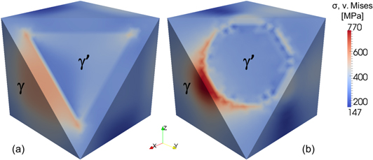
Figure 5. Full fields of equivalent von Mises stresses in the RVE with a cubic  precipitate (a) and a spherical
  precipitate (b) under uniaxial tensile load of 300 MPa in x-direction, respectively. The volume fraction of precipitate is approx. 40% and the lattice mismatch ratio is −0.0015. These stresses are calculated by FFT method without the subdivision of regions.
Download figure:
Standard image High-resolution imageMaking use of the same FFT method and equation (5) with the same model parameters, the full fields of plastic strains in the RVE with approx. 40% volume fraction of a spherical  precipitate for different loading conditions in a certain time step are obtained, which are shown in figure 6. By analyzing the geometrical symmetry and the similarity of deformation behavior, as well as considering the efficiency and accuracy of the calculation of internal stresses, the RVE with a spherical
  precipitate is divided into 10 regions as shown in figure 7. Thus, internal stresses can be calculated by equation (9) as
This is a simplified equation similar to equation (7). In fact, the whole effective stiffness matrix contains 60 × 60 components.
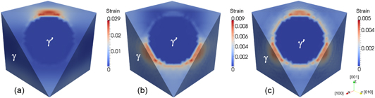
Figure 6. Full fields of equivalent plastic strains in 500 time steps in the RVE with a spherical  precipitate under a constant uniaxial tensile load of 300 MPa along [001] direction (a), [110] direction (b) and [111] direction (c).
Download figure:
Standard image High-resolution image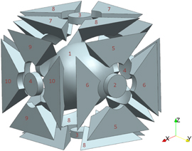
Figure 7. Schematic diagram of subdivision of RVE with a spherical  precipitate. The numbers indicate different regions.
Download figure:
Standard image High-resolution imageAs the expense of a certain accuracy, the subdivision method overcomes the limit of the computer memory for a long-time full field calculation and increases the efficiency. The subdivisions for two shapes of  phase proposed in our paper are only two of feasible ways. If the more accurate solution is required, a more complex subdivision can be made by the analysis of specific local stresses and deformations.
3. Validation of the effective stiffness matrix
3.1. Comparison of internal stresses
We assume that the volume fraction of  precipitate is approx. 66% and the total number of FFT grids in the RVE with a cubic
  precipitate is 32 × 32 × 32. Thus, the precipitate occupies 28 × 28 × 28 grids and each channel occupies 28 × 28 × 4 grids. Based on this microstructure and elastic constants [28], the effective stiffness matrix with 24 × 24 components can be determined. Since various loading conditions give rise to distinct eigenstrains in the RVE, we assigned many different values to eigenstrains to validate the reliability of equation (7) with the effective stiffness matrix. Here, we purposefully take arbitrary large eigenstrains shown in table 2 as an example to demonstrate the generality of our method. The calculated internal stress fields by FFT method are shown in figure 8. The corresponding effective values in the four sections of the RVE determined by averaging the FFT results within these regions are listed in table 3. The calculated internal stresses by effective stiffness method are listed in table 4. These internal stresses calculated by two methods are almost equivalent. Table 5 shows that the deviation of each stress component in the RVE between two methods, which is the absolute percentage of difference of individual stress component between two methods accounting for the corresponding stress component determined by FFT method. It can be seen that the maximum and average deviations are approx. 5.9% and 0.7%, respectively. Although the maximum difference of individual stress component could be in the order of 103 MPa for these given large eigenstrains, the deviation is small. If the magnitude of eigenstrains decreases, the value of internal stresses will decrease and the maximum difference of internal stresses would be smaller than 10 MPa which is negligible.

Figure 8. Calculated internal stress fields in the RVE with a cubic  precipitate by FFT method, where a local internal stress value is defined in every grid point.
Download figure:
Standard image High-resolution imageTable 2.
Assigned eigenstrains in the four sections of RVE with a cubic  precipitate.
| Strain component | 11 | 22 | 33 | 12 | 13 | 23 |
|---|---|---|---|---|---|---|

|
0.7 | 0.8 | 0.9 | 0.8 | 0.7 | 0.6 |

|
0.5 | 0.4 | 0.3 | 0.2 | 0.1 | 0.0 |

|
1.0 | 0.1 | 0.2 | 0.3 | 0.4 | 0.5 |

|
0.1 | 0.2 | 0.3 | 0.4 | 0.5 | 0.6 |
Table 3.
Effective internal stresses (MPa) in the four sections of RVE with a cubic  precipitate obtained by averaging FFT results within these regions.
| Stress component | 11 | 22 | 33 | 12 | 13 | 23 |
|---|---|---|---|---|---|---|

|
0.351e + 04 | −0.108e + 06 | −0.111e + 06 | −0.657e + 04 | −0.114e + 05 | −0.508e + 04 |

|
−0.372e + 05 | 0.780e + 04 | −0.714e + 04 | −0.162e + 04 | 0.876e + 05 | 0.827e + 04 |

|
−0.103e + 06 | −0.172e + 05 | 0.745e + 04 | 0.232e + 05 | −0.893e + 04 | 0.415e + 04 |

|
0.212e + 05 | 0.191e + 05 | 0.178e + 05 | −0.318e + 04 | −0.124e + 05 | 0.282e + 03 |
Table 4.
Calculated internal stresses (MPa) in the four sections of RVE with a cubic  precipitate by effective stiffness method.
| Stress component | 11 | 22 | 33 | 12 | 13 | 23 |
|---|---|---|---|---|---|---|

|
0.359e + 04 | −0.108e + 06 | −0.110e + 06 | −0.657e + 04 | −0.114e + 05 | −0.478e + 04 |

|
−0.371e + 05 | 0.786e + 04 | −0.697e + 04 | −0.162e + 04 | 0.878e + 05 | 0.827e + 04 |

|
−0.103e + 06 | −0.171e + 05 | 0.750e + 04 | 0.234e + 05 | −0.893e + 04 | 0.414e + 04 |

|
0.213e + 05 | 0.191e + 05 | 0.178e + 05 | −0.318e + 04 | −0.124e + 05 | 0.279e + 03 |
Table 5.
The deviation (%) of the internal stresses in the four sections of RVE with a cubic  precipitate between the results obtained by FFT method and effective stiffness method.
| Stress component | 11 | 22 | 33 | 12 | 13 | 23 |
|---|---|---|---|---|---|---|

|
2.3 | 0.0 | 0.9 | 0.0 | 0.0 | 5.9 |

|
0.3 | 0.8 | 2.4 | 0.0 | 0.2 | 0.0 |

|
0.0 | 0.6 | 0.7 | 0.9 | 0.0 | 0.2 |

|
0.5 | 0.0 | 0.0 | 0.0 | 0.0 | 1.0 |
When the volume fraction of  precipitate changes, the average deviation varies a little, but the fluctuation of maximum deviation is larger, as shown in figure 9. There is no monotonic regulation between deviations and volume fractions. Nevertheless, these deviations are generally acceptable. Furthermore, if the precipitate is a cuboid, which occupies 28 × 30 × 26 grids, the maximum and average deviations are approx. 6.8% and 0.6%, respectively. Therefore, the simple effective stiffness method is valid for calculation of internal stresses in both cubic and cuboid cases with different volume fractions of
  precipitates, and the accuracy increases with decreasing magnitude of eigenstrains.
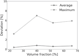
Figure 9. The average and maximum deviations of calculated internal stresses in the RVE with a cubic  precipitate between FFT method and effective stiffness method as a function of volume fractions of
  precipitate.
Download figure:
Standard image High-resolution imageWhen we use different elastic constants of γ and  phases [13] to redo the calculation for cubic precipitate with 66% volume fraction, the maximum and average deviations are approx. 2.9% and 0.4%, respectively. This demonstrates that the unequal elastic constants for two phases do not worsen the accuracy of this new method, and the same indication is also found for other volume fractions.
For given arbitrary values of eigenstrains in the 10 sections of the RVE with a spherical  precipitate as shown in table 6, the maximum and average deviation between FFT method and effective stiffness method are approx. 4.7% and 0.4%, respectively, as displayed in table 7. The influence of volume fractions is shown in figure 10. It is found that for volume fraction of 20%, one stress component has a large deviation, however, its absolute difference is only 25 MPa. Furthermore, the assigned eigenstrains in this paper are complex, which may increase the deviation. The calculated internal stresses would be more accurate in the simple deformation case. Hence, the effective stiffness method is also available to obtain the reasonable results for spherical
  precipitates.
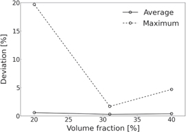
Figure 10. The average and maximum deviations of calculated internal stresses in the RVE with a spherical  precipitate between FFT method and effective stiffness method as a function of volume fractions of
  precipitate.
Download figure:
Standard image High-resolution imageTable 6.
Assigned eigenstrains in the 10 sections of RVE with a spherical  precipitate.
| Strain component | 11 | 22 | 33 | 12 | 13 | 23 |
|---|---|---|---|---|---|---|

|
0.5 | 0.1 | 0.5 | 0.7 | 0.04 | 0.05 |

|
−0.1 | 0.0 | 0.3 | 0.8 | 0.8 | 0.0 |

|
0.3 | 0.4 | −0.4 | 0.1 | 0.2 | 0.07 |

|
0.2 | −0.2 | 0.0 | 0.0 | 0.1 | 0.01 |

|
0.5 | −0.2 | 0.0 | 0.1 | 0.0 | 0.08 |

|
0.2 | 0.0 | 0.0 | −0.2 | 0.7 | 0.0 |

|
0.3 | 0.0 | −0.2 | 0.4 | 0.0 | 0.0 |

|
0.0 | 0.2 | 0.5 | 0.05 | −0.6 | 0.0 |

|
0.4 | 0.3 | 0.4 | 0.7 | 0.0 | 0.0 |

|
0.4 | 0.4 | 0.0 | 0.007 | 0.3 | 1.0 |
Table 7.
The deviation (%) of the internal stresses in the 10 sections of RVE with a spherical  precipitate between the results obtained by FFT method and effective stiffness method.
| Stress component | 11 | 22 | 33 | 12 | 13 | 23 |
|---|---|---|---|---|---|---|

|
0.0 | 0.4 | 0.0 | 0.5 | 0.2 | 0.2 |

|
0.6 | 0.2 | 0.8 | 0.2 | 0.2 | 0.3 |

|
4.7 | 0.5 | 0.8 | 0.0 | 0.0 | 0.0 |

|
0.2 | 0.0 | 0.0 | 0.5 | 0.3 | 1.8 |

|
0.0 | 0.0 | 0.0 | 0.5 | 0.0 | 0.0 |

|
0.0 | 0.0 | 0.0 | 0.4 | 0.1 | 0.0 |

|
0.4 | 0.7 | 0.2 | 0.0 | 0.0 | 0.3 |

|
0.4 | 0.0 | 1.5 | 0.9 | 0.0 | 0.2 |

|
0.0 | 0.2 | 0.0 | 0.8 | 0.0 | 0.2 |

|
2.3 | 0.0 | 0.7 | 0.2 | 0.0 | 0.1 |
3.2. Comparison of plastic strains
Following the present subdivision and assigning the internal stresses in different regions obtained by the FFT method or the effective stiffness method to equation (5), the plastic strain in each region in every time step can be calculated. Thus, the general equivalent plastic strain of RVE is given by

where fi and  are the volume fraction and the equivalent plastic strain of each region i, respectively, and m is the total number of regions. The used model parameters are the same as that in table 1. Figure 11 shows that the comparisons of the equivalent plastic strains for different methods in some typical regions of the RVEs with a cubic
  precipitate and a spherical
  precipitate, respectively, which demonstrates that the FFT method and the effective stiffness method almost lead to the same results, where small deviations occur at rather large strains. For [110] and [111] loading conditions, the general equivalent plastic strains obtained by two methods are nearly identical as shown in figure 12. These results denote that, in general, the deviation increases with increasing strain. This is consistent with the previous indication that the accuracy of internal stresses calculated by the effective stiffness method decreases with increasing magnitude of eigenstrains. Moreover, the deviation in the case of a cubic precipitate is larger than that in the case of a spherical precipitate for the same strain. Due to the more subsections in the RVE with a spherical precipitate, the description of the stress states is improved, so that the precision is enhanced.
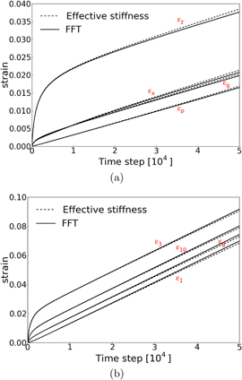
Figure 11. Equivalent plastic strains in the RVE with a cubic  precipitate (66% volume fraction) (a) and a spherical
  precipitate (40% volume fraction) (b) as a function of the time step under a constant uniaxial tensile load of 300 MPa along [001] direction, obtained by FFT method and effective stiffness method, respectively.
Download figure:
Standard image High-resolution image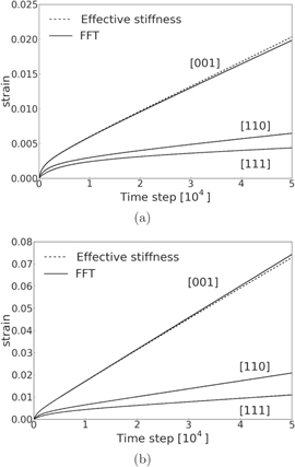
Figure 12. Comparisons of the general equivalent plastic strains between the results obtained by FFT method and effective stiffness method in the RVE with a cubic  precipitate (66% volume fraction) (a) and a spherical
  precipitate (40% volume fraction) (b) as a function of the time step under a constant uniaxial tensile load of 300 MPa along [001], [110], and [111] directions, respectively.
Download figure:
Standard image High-resolution image4. Application in crystal plasticity FE model
4.1. Crystal plasticity constitutive equations
Based on the dislocation slip controlled phenomenological crystal plasticity model [29], a new flow rule for  slip in each γ matrix channel is

where α represents the slip system,  is the shear rate in a certain slip system,
  is the reference shear rate,
  is the Orowan stress, and p1 is the inverse value of the strain rate sensitivity. The resolved shear stress
  is given by

where  is the elastic deformation gradient, and
  is the Schmid matrix. The internal stress gives rise to an additional resolved shear stress as

 is the slip resistance determined by
where β is the slip system, h0 is the reference hardening parameter,  is the cross hardening matrix,
  is the saturated slip resistance due to dislocation density accumulation, and p2 is a fitting parameter. Due to the shearing of
  precipitate by stacking faults [7, 16], the flow rule for
  slip in
  precipitate is

Taking the RVE with a cubic  precipitate as an example, the plastic velocity gradients in the four subsections as discussed above are given by


With the known plastic deformation gradient in the previous time step, the current plastic deformation gradients for different regions are


and the total plastic deformation gradient  is calculated by

where  ,
,  ,
,  , and
, and  are volume fractions of each γ channel and precipitate, respectively.
  is the time step. The eigenstrains in each subsection originated from the plastic deformation gradients are


The internal stresses can be determined from these eigenstrains at each time step by equation (7) efficiently. The same method is able to be used for the RVE with a spherical  precipitate.
4.2. FE model
The crystal plasticity constitutive equations are able to be implemented in the ABAQUS [30] platform by using a user-defined subroutine UMAT. A simple 3D FE model with dimensions of 80 mm × 40 mm × 40 mm is set up to represent a sample of single crystal superalloys. As shown in figure 13, the 1/8 complete sample is discretized with 2000 regular C3D8 elements, in which each integration point is represented by the previous RVE. The symmetric boundary conditions are applied in x-, y-, z-direction, respectively. The common model parameters are shown in table 8. According to different shapes and volume fractions of  precipitate, as well as different γ channel widths,
  can be determined by the Orowan threshold equations proposed in [13, 31]. Assuming the volume fraction of
  precipitate is 40% and the length of the RVE is 500 nm, the Orowan stresses are 71 MPa and 22 MPa for cubic
  and spherical
  precipitates, respectively.
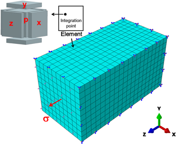
Figure 13. The 1/8 3D finite element model with boundary conditions.
Download figure:
Standard image High-resolution imageTable 8.
Crystal plasticity model parameters.  is the initial slip resistance.
 (s−1) (s−1) |

|
 (MPa) (MPa) |
60 |
 (MPa) (MPa) |
500 |
| p1 | 10 |
| p2 | 0.05 |
| h0 (MPa) | 60 |
 (MPa) (MPa) |
800 |
 coplanar{111} coplanar{111} |
1.0 |
 non-coplanar{111} non-coplanar{111} |
1.4 |
| δ | −0.0015 |
Loading in z-direction (i.e., [001] crystallographic orientation) with a constant stress of 300 MPa for  s, the sample deforms almost homogeneously and the plastic strain evolving with time is displayed in figure 14. Since the internal stresses in the whole sample are nearly same, we select one arbitrary element to show the evolution of internal stresses during the deformation. For the cubic
  precipitate, from figure 15(a), it can be seen that the internal stresses in γ channels decrease in the beginning and increase gradually afterwards, but the internal stress in the precipitate increases continuously. Initially, the internal stresses are determined by the lattice mismatch. The following deformation accommodates the misfit strain first, so that the high internal stresses in channels decrease. This is also observed in the full field calculation shown in figure 1(b). However, when they reach certain values, they will increase again, because the further accumulation of deformation in the microstructure will cause the increase of internal stresses. In addition, due to the high strength of
  precipitate, the inhomogeneous deformation in the channels and the precipitate leads to increasing internal stresses. The previous deformation state determines the current internal stresses, the current internal stresses influence the further deformation as well. The similar phenomenon of internal stresses during the creep in the superalloy has been discussed in [32]. For the spherical
  precipitate, the evolution of internal stresses is shown in figure 15(b). It is found that the different shapes of
  precipitates result in different internal stresses which give rise to different plastic strains. Our method can discriminate the influence of the various shapes of
  precipitate on deformation behavior for the same volume fraction.

Figure 14. The plastic strain as a function of time under uniaxial tensile load of 300 MPa in z-direction for single crystal superalloys with cubic  and spherical
  precipitates, respectively.
Download figure:
Standard image High-resolution image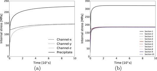
Figure 15. The von Mises internal stresses in one element for the cubic  precipitate (a) and the spherical
  precipitate (b) as a function of time under uniaxial tensile load of 300 MPa in z-direction.
Download figure:
Standard image High-resolution image
The present FE model is one simple application of our effective stiffness method. The detailed analysis of deformation in this model is not the focus of this paper. In the future, the effective stiffness method can be used in more complex and more realistic models, in which the simulation results are able to rationalize the experimental observations.
5. Conclusions
On the basis of typical γ/γ' microstructures of superalloys, the internal stresses due to eigenstrains resulting from lattice mismatch and deformation heterogeneity can be calculated by an efficient linear relation with an effective stiffness matrix. The effective stiffness method can be considered as a generalization of the Eshelby inclusion problem for more complex microstructures. It relies on a subdivision of the microstructure into regions with uniform deformation behavior. The feasibility of such a subdivision has been demonstrated for γ/γ' microstructures with cubic and spherical precipitates. Compared with direct simulations with the FFT method, which determines the internal stress fields with the full spatial resolution, this simplified method is numerically much more efficient and thus well suitable for applications in macroscopic simulations of deformation and creep with FE method or other mechanics solvers. The effective stiffness matrix is calculated by the FFT method and its dimension varies with different morphologies of  precipitates. The accuracy of this method increases with decreasing magnitude of eigenstrains, but it is not significantly influenced by the volume fraction of
  precipitate and elastic constants. Furthermore, if the volume fraction and shape of
  phase in superalloys remain unchanged during the deformation, the effective stiffness matrix will be constant throughout the simulation.
Acknowledgments
The authors are grateful for funding by the Deutsche Forschungsgemeinschaft (DFG) through Project C4 of the collaborative research center SFB/Transregio 103 superalloy single crystals under grant number INST 213/747-2.