

Abstract
Laser distance sensors are a widespread, fast and contactless approach for distance and surface topography measurements. Main characteristics of those sensors are given by resolution, measurement speed and sensor geometry. With decreasing sensor size, the alignment of the optical components in sensor setup becomes more challenging. The depth response of optical profilers is analyzed to obtain characteristic parameters and, thus, to value the alignment and the transfer behavior of those sensors. We present a novel miniaturized sensor setup comprising of confocal and interferometric confocal signals within one sensor in order to compare both principles simply by obscuring the reference arm by an absorber. Further, we introduce a theoretical signal modeling in order to analyze influences such as spatial coherence, Gaussian beam characteristics and tilted reflectors on depth response signals. In addition to this, we show that the coherent superposition significantly reduces the axial resolution due to the confocal effect in interferometric signals compared to simple confocal signals in measurement and simulation results. Finally, an appropriate fit function is presented, in order to figure out characteristic sensor parameters from the obtained depth response signal. In this context, a good agreement to simulated and measured signals is achieved.
Export citation and abstract BibTeX RIS

Original content from this work may be used under the terms of the Creative Commons Attribution 4.0 license. Any further distribution of this work must maintain attribution to the author(s) and the title of the work, journal citation and DOI.
1. Introduction
In order to achieve a fast and contactless measurement of surface profiles on the micro- and nanoscale, optical point sensors are combined with appropriate scan axes [1–5]. Besides profilometry, point-wise measuring distance sensors are also used e.g. for nanopositioning [6, 7] and error compensation [8, 9] integrated in complex measurement systems. Commonly requested sensor properties are small geometrical dimensions of the probe, high lateral resolution, low axial measurement uncertainty and high measuring velocities. Compared to conventional microscopic arrangements, confocal microscopes lead to a better lateral and axial resolution, which is a consequence of pinholes applied for illumination and detection. The confocal filtering effect is usually considered in an optical point sensor due to the use of a single-mode fiber for illumination and detection [10–12]. Further, the axial resolution is improved as a result of phase analysis using an interference arrangement.
With decreasing sensor size the demands on the alignment of sensor components increase. For each individual component minor changes in its location or tilt are crucial with respect to the beam alignment. In order to validate the beam alignment and to characterize the sensor by parameters such as the numerical aperture (NA), depth response signals can be analyzed by comparisons with results obtained by simulation models. Simulations enable a precise development of measured depth response signals [4, 13–17], since various effects and their impact on the signal can be assessed isolated in theoretical viewing [18, 19]. In previous studies various influences such as spherical aberrations and different pinhole sizes are included in theoretical models and investigated in detail [20, 21]. Therefore, theoretical studies can be used in order to optimize the arrangement of optical components in the sensor and further to identify systematic deviations and their causes contribute to sensor optimization.
In this study, a miniaturized fiber optical point sensor is presented. The sensor is able to perform confocal and interferometric confocal measurements subsequently by adding an optical absorber in the optical path of the reference arm. This allows a direct comparison between the depth response signals obtained by these sensor configurations. With the help of simulations differences between the respective interferometric and non-interferometric signals are investigated. Based on these investigations, several effects occurring in measured signals are shown and analyzed. Further, the influence of a tilted reflector surface is included in the theoretical modeling of the sensor's response signal. As shown, the theoretical modeling is useful to draw a conclusion about the sensor alignment. In addition, to the best of our knowledge, a new approach is used to extract special parameters, such as the NA or the depth of field (DOF), from a measured depth response signal by using a fit function. The fit function is obtained from a theoretical approach combining the sum of two axial intensity profile functions. These intensity profile functions are designed with characteristic measurement parameters to determine these parameters directly from the fit function. Characteristic parameters extracted from the fit function are confirmed by comparative measurement results obtained from a chirp standard using the presented sensor and an AFM.
2. High-speed laser distance sensor
This section deals with a point-wise measuring distance sensor built to perform height measurements on surfaces with structures in the micro- and nanometer range [5]. A schematic illustration and a related photograph of this sensor are depicted in figure 1. As shown in figure 1(a), a laser beam is emitted from the end-face of an optical single-mode fiber and then collimated by a gradient-index (GRIN) lens. This beam is split by a beam splitter cube (with geometrical dimensions of 5 mm × 5 mm × 5 mm) in a measurement and a reference arm, where these beams are focused by equal aspherical lenses onto the surface to be measured and an ultrasonic transducer acting as reference mirror, respectively. The reflected beams are superimposed at the beam splitter, collected by the single-mode fiber and finally converted by a photodiode in an electrical signal for subsequent processing and analyzing. Due to a prism mirror in the reference arm, measurement and reference arm are balanced without a significant increase of the sensor dimensions. Furthermore, an absorber can be placed in the reference arm, which enables to switch between an interferometric confocal and an exclusively confocal sensor configuration. For this reason the sensor is called hybrid sensor in the following. An oscillation of the reference mirror at ultrasonic frequencies in axial direction leads to a modulation of the optical path length difference, what is used to determine height values by a phase evaluation algorithm, as discussed in more detail by Hagemeier et al [5].
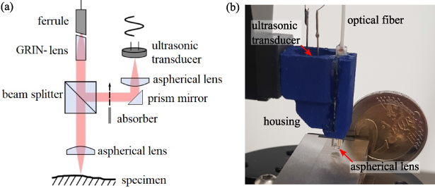
Figure 1. Schematic illustration (a) and photograph (b) of the fiber-coupled hybrid sensor with geometrical dimensions of approx. 12 mm × 25 mm × 17.5 mm (width × height × depth).
Download figure:
Standard image High-resolution imageSince the main part of this contribution focuses on theoretical and practical investigations of the sensor depth response, only depth scans are performed with this sensor and thus, no height values are acquired for comparison to theoretical investigations. The depth scan is performed using a linear stage vertically aligned in a multisensor measuring system [22], where the distance between sensor and surface under investigation continuously decreases, while the interference signal is captured by a photodiode. The resulting signal can be used to characterize the sensor as discussed in the following sections.
3. Basic composition of depth response signals
This section introduces a simulation model of confocal and interferometric confocal depth response signals on the basis of Fourier optics. For the sake of simplicity we use a scalar approach which leads, in case of depth response signals, to similar results as a vectorial treatment [15, 23]. In confocal microscopy the light passing the pinhole, which is given by the the front face of the single-mode fiber core in the sensor setup presented above (see figure 1), can be approximated by a point light source. Since point light sources are spatially coherent, the total intensity captured by the detector can be described by the absolute square of the integral of the electric fields in contrast to a spatially incoherent light source, where the intensities superimpose in the detector [14]. Thus, the intensity  of a confocal depth signal depending on the defocus z obtained from a perfect plane mirror is given by
where  is the axial wave vector component with the angle of incidence θ and the wave number
  related to the wavelength
  [15, 24]. The maximum incident angle
  is restricted by the NA of the aspherical focusing lens (see figure 1). Inhomogeneous pupil illumination and apodization effects can be considered by the pupil function
  . In the first part of this study
  is assumed for simplicity matching the case of a homogeneously illuminated pupil without apodization. Afterwards,
  is replaced by a Gaussian function in order to include the properties of the illuminating laser light source. Note that the pinhole is approximated to be infinitely small. Considering a finite sized pinhole with the radius R of the fiber core, the pupil function needs to be multiplied by a low-pass filter
  of the form
with the Bessel function J1 of first kind and order, since the single-mode fiber acts as a coherent detector [11, 18].
In the paraxial approximation  can be assumed and the integral can be solved analytically, leading to the intensity [15]
Since small angles of incidence are assumed, the paraxial approximation is valid for small NA values.
In case of interferometric confocal signals equation (1) is extended to [15]
where the reference mirror is assumed to be a perfectly reflective plane mirror in the focal plane at z = 0 resulting in  . Considering realistic materials, both, the object and the reference arm must be multiplied by angle dependent reflection coefficients.
Figure 2(a) shows the depth response signals of the confocal and interferometric confocal sensor according to equations (1) and (4). For a better visibility of the interference fringes within the DOF a larger NA of 0.6 is chosen, compared to the smaller NA value of the sensor used in practice. The shape of the confocal signal shows a maximum peak in the focal position and approximately follows the shape of a sinc2 function. The envelope of the interference signal seems to be broadened compared to the confocal signal. Thus, the reference obviously counteracts to the constriction resulting from the confocal effect. The influence of interference on the envelope will be discussed in detail in the results (see section 4).
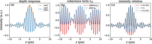
Figure 2. (a) Confocal and interferometric confocal depth response signal. (b) Impact of the coherence term  on the interferometric depth response signal compared to incoherent superposition for
  and
and  . (c) Different ratios of object intensity I and reference intensity
  . Note that an offset is subtracted from the interference intensities.
Download figure:
Standard image High-resolution imageFurther, the envelope of the interferometric signal shows an asymmetry with respect to positive and negative interference intensity values. Note that the interference intensity is reduced by an offset and hence, negative intensity values occur. In case of spatially incoherent illumination, symmetric interference intensities are expected. Thus, the asymmetry follows from spatially coherent illumination as it will be demonstrated in the following. For simplicity, the influence of a spatially coherent light source on the interference signal is explained considering the superposition of only two coherent illuminating electromagnetic waves with the axial wave numbers  and equal amplitudes resulting in the total electric field distribution

Note that the terms varying in z-direction follow from the object arm, i.e. the optical path difference. The intensity I measured by the detector is proportional to the absolute square of  leading to

which is composed by an offset, two cosine functions and the coherence term  . Neglecting
  , the interference intensity would correspond to the case of spatially incoherent superposition. Hence,
  constitutes the difference between spatially coherent and incoherent illumination.
Figure 2(b) shows the offset reduced intensities with and without the term  . The envelope of the intensity without
  shows symmetry with respect to the z-axis, whereas the coherent superposition leads to an asymmetry. Therefore, the decreased modulation with regard to negative interference intensities and enhanced modulation for positive interference intensities can be explained by the additional cosine term caused by coherent illumination. It should be mentioned that the periodicity of the functions follow from the smaller unambiguity range as solely two frequencies contribute.
Figure 2(c) displays interferometric confocal depth responses for different amplitude ratios between measurement and reference wave. The asymmetry is reduced, if the amplitude of the reference wave is increased compared to the amplitude of the wave from the object under investigation and increased for smaller reference amplitudes or higher amplitudes of the object wave. Thus, the asymmetry can be influenced by changing the amplitudes of the waves reflected from the surfaces of the reference and measurement object.
Since the lateral beam profile of light in a single-mode fiber is approximately described by a Gaussian distribution [25], the theoretical model is extended by a Gaussian beam instead of a homogeneously illuminated pupil. Therefore, the pupil function  in equation (1) is replaced by a Gaussian function of the form
with the radial wave number component  . The parameter a defines the fraction of intensity of the Gaussian function at the NA limit of the pupil. For example, a homogeneous pupil illumination is described by
  . If
. If  , the illuminating intensity at
  is 0.1 of the maximum intensity. Since we are finally interested in an appropriate fit function in order to extract parameters from measured signals, we first focus on confocal signals in the following investigation.
The intensity  of a confocal depth response considering Gaussian illumination is described by
According to Gaussian beam theory, the axial intensity profile of a Gaussian laser beam is given by a Lorentzian function
where  defines the Rayleigh length [26–28]. The depth response signal for homogeneous illumination can be approximated by equation (3) in the paraxial case. As the NA of the sensor presented in this study is assumed to be between 0.2 and 0.3, the paraxial approximation is justified. Therefore, a new approach inspired by the Pseudo-Voigt profile [29] is introduced with

where equations (9) and (3) are superimposed and weighted with q and  for
for  , respectively. More precisely, the signal can be written as the convolution of L(z) and
  . However, fitting a convolution leads to a slow convergence of the fit function and, thus, equation (10), in the following referred to as SL-function, is used analogously to the Pseudo-Voigt profile. Figure 3 displays the depth response signal computed numerically according to equation (8) for a Gaussian illumination with a = 0.3 following equation (7). The simulated depth response is approximated by three fit functions, a Lorentzian (equation (9)), a sinc2 (equation (3)) and the SL-function defined by equation (10). A comparison shows that the SL-function is in good agreement to the simulated signal, whereas the Lorentzian as well as the sinc2 function exhibit significant deviations. Furthermore, the
  extracted from the fit corresponds to the NA of 0.2 prescribed in the simulation. This opens the possibility to gain parameters from measured depth response signals and, thus, to characterize confocal sensors. In addition, the Rayleigh length and the weighting factor q provide information about the quality of the laser beam, if the function is used in order to analyze measured results on the basis of depth response signals. Further, the theoretical model can be extended considering misalignment effects and consequently, influences on the confocal depth response signal can be investigated. As an example for misalignment, we study the impact of tilting the sensor with respect to the normal to the surface. However, various disturbances and aberrations can be included into the model analogously to [15, 30–32].
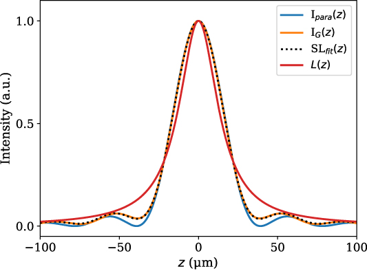
Figure 3. Theoretical depth response signal  as defined in equation (7) together with the approximated SL fit (equation (10)), a fitted sinc2 function according to
  (equation (3)) and a Lorentzian fit function L(z) (equation (9)) for λ = 1550 nm, a = 0.3, NA = 0.2 and q = 0.13.
Download figure:
Standard image High-resolution imageIn order to extend the confocal model of equation (1) to tilted specular surfaces, the scattering geometry can not be treated as rotationally symmetric anymore. Hence, the incident wave vector is considered in the conical form
with the incident angle  with respect to the z-axis and the azimuth angle
  in the xy-plane. Considering a tilted surface, with the tilt angle
  with respect to the x-axis according to figure 4(a), the x-component
  of the incident wave vector can be rewritten to
where
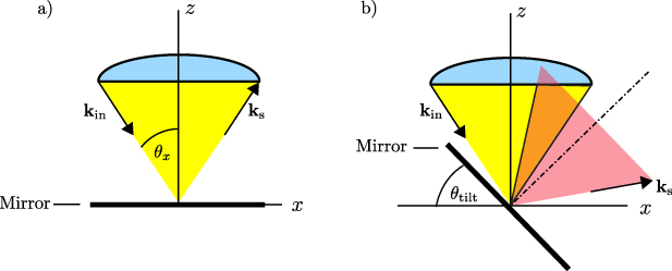
Figure 4. Schematic illustration of the incident (yellow) and scattered (red) light cone on a (a) perfectly aligned plane mirror, (b) tilted plane mirror.
Download figure:
Standard image High-resolution imageis the incident angle of the projection of  into the xz-plane as sketched in figure 4(a). Therefore, the scattered or reflected wave vector results in
Since the mirror is only tilted in the xz-plane,  is unchanged. Due to the tilt of the scattered light cone (see figure 4(b)), equation (1) is multiplied by a further filter function
leading to the detected intensity
Equation (15) considers that not each scattered ray is collected by the aspherical lens.
Figure 5 presents simulated depth response signals obtained for three different tilt angles. In figure 5(a) the signals are normalized by their own maximum value, in figure 5(b) they are normalized by the maximum value obtained for the perfectly aligned plane mirror. As expected, the signals are broadened and the maximum intensity decreases with increasing tilt angles, because the intensity, which is not captured by the aspherical lens ( in equation (15)) increases as demonstrated schematically in figure 4(b). Thus, the effective NA and the maximum intensity of the depth response signal decreases for tilted surfaces. However, since the maximum intensity decreases with tilts between the sensor and the surface, the focal intensity can be consulted as a measure for the alignment.
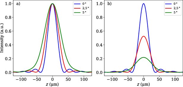
Figure 5. (a) Axial depth response signals for different tilt angles of the perfectly reflecting object calculated for an NA of 0.2 of the focusing lens placed in the measurement arm normalized by the respective maximum intensity value. (b) Intensities normalized by the maximum intensity related to the perfectly aligned specimen to show the loss of reflected light due to the tilt angle.
Download figure:
Standard image High-resolution image4. Results
4.1. Depth response
In this section signals of the presented hybrid sensor are shown and compared to simulated results. As presented in figure 2(a), in theory there are two remarkable differences between the confocal and interferometric confocal signals: The broadened interference envelope compared to the confocal signal and an asymmetry between the zero-mean positive and negative interference intensity values. Here, one of the main advantages of the hybrid sensor come into play. With the help of the hybrid sensor, first a confocal and afterwards an interferometric confocal measurement is obtained. Therefore, measurements are performed under the same conditions, meaning the use of equal hardware, software and almost the same environmental conditions. Even the lateral position of the measurement point on the surface under test, the scan velocity and the starting distance of the depth scan are the same.
The results of both measurements are shown in figure 6(a). Compared to simulated results (figure 6(c)), the measured depth responses are superimposed by noise. Due to the smaller NA values compared to figure 2, single fringes are not visible in the interferometric signals because of the large DOF. Further, the measured intensities are reduced by an offset. The interference intensity in case of the measured result almost shows symmetry with respect to the z-axis. According to figure 2(c), this could be due to different intensities captured from the object and reference arm. In order to compare the envelopes occurring with and without reference wave, the measured signals are band-pass filtered and the envelope of the interference signal is determined using the Hilbert transformation analogously to [33]. The measured envelopes are displayed in figure 6(b). Similar to the simulated depth responses (figure 6(c)), the interferometric envelope is broadened with respect to the confocal signal. Thus, this effect can be confirmed by simulation and therefore probably simply follows from interference.
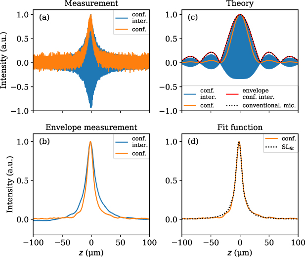
Figure 6. (a) Experimental offset-reduced confocal and interferometric confocal depth response signals of the hybrid sensor. (b) Envelopes of the measured signals. (c) Signal and envelopes of the theoretical models including the depth response signal of a conventional microscope for  . (d) Measured confocal signal and fitted SL-function.
Download figure:
Standard image High-resolution imageIn figure 6(c) the envelope of the simulated interference signal does not exactly fit the interference fringes. This is caused by the asymmetry of the interference fringes discussed in section 3. Furthermore, the envelope expected from a conventional microscope, which equals to those of coherence scanning interferometers, is approximated by the square root of the confocal envelope as shown by Kino et al [15]. Note that the envelope of the interferometric confocal signal in figure 6(c) matches the signal of a conventional microscope, which leads to the assumption that the confocal effect does not improve the axial resolution as given by the envelope of an interferometric confocal sensor. Probably, the confocal effect leads to an increase of constructive interference and an decrease of destructive interference, what in average cancels to the envelope of a conventional microscope. Note that the side lobes in figure 6(c) are not observable in figures 6(a) and (b). This can be explained by a higher contribution of the Lorentz function (q = 0.67) in the measurement result (figures 6(a) and (b)) compared to the simulated response signal approximating a homogeneously illuminated pupil depicted in figure 6(c).
Figure 6(d) shows the depth response of the confocal sensor according to figure 6(c) and the fitted SL-function (see equation (10)). Apart from small deviations caused by aberrations, the approximated fit function shows good agreement with the measured result. The NA resulting from the fit is given by 0.21. Since the NA of the aspherical lens amounts to 0.58, the pupil does not seem to be fully illuminated. This effect could be confirmed using the optic design software OpticsStudio by Zemax [34]. Therefore, in future studies, the sensor can be improved changing the GRIN lens in order to achieve a more uniform pupil illumination and hence a higher NA value. However, the measured signal is well approached by the SL-function, which enables to extract parameters such as the NA from measured depth response signals. Thus, this fit is shown to be an useful tool for sensor characterization.
4.2. Chirp standard
In order validate the previously determined NA value, a measurement using the interferometric confocal distance sensor (ICDS) is obtained from a fine chirp structure. The fine chirp structure manufactured by PTB (Physikalisch-Technische Bundesanstalt, Germany) exhibits nominal peak-to-valley amplitudes of 400 nm and nominal spatial wavelengths between 3.8 and 12 μm [35, 36]. Besides the profile measured by ICDS, an additional profile is measured by the Nanite AFM from Nanosurf [37] using the cantilever Tap190Al-G from BudgetSensors [38]. In order to determine the NA from the measured chirp structure, the profile obtained by the AFM is convolved with a time-limited function corresponding to a moving average filter with the window width  . If the surface under investigation is located in the DOF of the ICDS, the window width can be approximated by the minimum waist w0 of the Gaussian beam to [5]
where  represents the lateral scan velocity and
  the frequency of the oscillating reference mirror.
  represents the fraction of a half period
  , which is as the evaluation window. While the second term considers the filtering by the lateral scanning process, the first term is twice the minimum waist of a Gaussian beam
In this relation, the confocal effect provoked by the fiber core is considered by the factor 0.75, which is determined by comparative measurements with an AFM using the fine chirp structure as measurement object in [36]. Assuming an NA value of 0.21, a scan velocity  = 20 mm s−1, an oscillation frequency
  = 40 kHz and 0.5 for
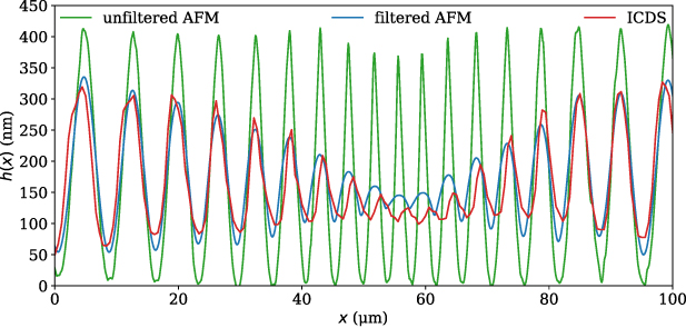
  a rectangular moving average filter applied to the profile measured by the AFM results in the blue profile depicted in figure 7. We apply a rectangular filter function as a rough approximation of the real shape of the filter. In comparison with the red profile measured by the ICDS with a lateral scan velocity of 20 mm s−1, the profile exhibits a similar constriction, which indicates that the NA of 0.21 determined using the depth response is sufficiently accurate. Note that the profile obtained by ICDS is determined by phase evaluation described in more detail in [5]. Deviations between the determined profiles may result from misalignments of the chirp structure orientation, different measurement locations on the chirp standard and not perfectly chosen values for the parameters of the filter function. Likewise, the determined factor of 0.75 representing the confocal effect is also an estimation. Therefore, further investigations using rigorous simulations, as for example used for coherence scanning interferometry [39] and confocal microscopy [40], promise to obtain more accurate results in order to determine correct parameters and to investigate the influence of the confocal effect.
Figure 7. AFM profile low-pass filtered (blue) and unfiltered (green) obtained from a fine chirp structure and filtered by a moving average filter with a window length corresponding to equation (17) compared to the profile (red) measured by the ICDS with a lateral scanning velocity of 20 mm s−1.
Download figure:
Standard image High-resolution image
Note that the characterization of the ICDS using the fine chirp standard is performed analogous to previous studies [5, 36]. In our study, characteristic sensor parameters are obtained by a depth scan. Since the confocal depth response signal is more familiar and straightforward to analyze compared to the confocal interferometric one, we use only the confocal signal for the sensor characterization. In order to verify the determined characteristic parameters, namely the minimum waist and the effective NA of the system, results obtained from the depth response signal are compared to those of a measured profile from a chirp standard. A depth scan is not necessary for profile measurements using the ICDS due to the oscillating reference mirror enabling a phase evaluation.
5. Conclusions
We present a novel hybrid laser point sensor that is able to perform confocal and interferometric confocal measurements under the same conditions using an absorber in the reference arm for switching between the two measurement modes. Comparing confocal and interferometric confocal results, an increasing DOF appears in the interferometric signal. Thus, the improvement of the axial resolution in the envelope signal caused by the confocal effect is reduced by the reference wave. This effect is confirmed by simulated depth response signals and can be explained by coherent superposition. Further, we demonstrate that coherent superimposition leads to an asymmetric interference intensity with respect to the depth axis in interferometric confocal signals. The influence of coherent superposition on the lateral resolution will be analyzed in future studies. Note that the response signal obtained by a depth scan moving the sensor axially is only necessary to characterize the sensor. Due to a height determination by phase evaluation using an oscillating reference mirror, the interferometric principle provides a much better axial accuracy compared to the confocal method. In addition, since there is no need for a mechanical depth scan the ICDS provides high data rates such as 116 000 height values per second as reported in [5].
Due to its small geometric dimensions and the possibility to adapt the probe in the measurement arm e.g. by a prism in front of the probe to achieve a 90∘ deflection of the focusing beam similar to [3, 41], the sensor can be applied in various fields of application (e.g. for surface profiling even in hard-to-access areas). However, small geometric dimensions lead to difficulties in the alignment of the optical components in the sensor setup. Therefore, we present a theoretical signal modeling and show that the confocal depth response signal is well approximated by superposition of a sinc2 and a Lorentzian function. Fitting this function to measured depth response signals, we are able to extract characteristic parameters such as the effective NA and the illuminating intensity distribution in the pupil plane. This is an important tool to assess the alignment and quality of the sensor setup.
Although a depth scan is not the typical operation mode of such sensors, depth scans are shown to be useful in order to extract sensor beam parameters and to validate the sensor alignment. Additionally, the theoretical model can be easily extended to include further disturbances as demonstrated by the example of a tilt between sensor and measurement object. Hence, disturbances in measured results can be identified in depth response signals by comparisons with simulated signals. The presented model can thus help to adjust these types of sensors and to identify or investigate the causes of disturbances occurring in measured signals. In addition, future developments aim to reduce the geometrical dimensions of the sensor and to improve the signal quality by changing optical components such as the GRIN lens and reference mirror. Therefore, the theoretical modeling turns out as an important means to ensure a proper sensor alignment.
Acknowledgments
The authors gratefully acknowledge the financial support of the research projects GZ: LE 992/14-1 founded by the Deutsche Forschungsgemeinschaft (DFG) and Zentrales Innovationsprogramm Mittelstand (ZIM) project ZF4126411DF8 founded by the Federal Ministry for Economic Affairs and Energy of Germany, which both contribute to the results presented in this collaborative study.
Data availability statement
The data that support the findings of this study are available upon reasonable request from the authors.