


Abstract
We describe here an artifact that may affect to magneto-optical Kerr measurements. When paramagnetic sample holders (SH) with non-negligible susceptibilities are used, the inhomogeneity of the applied magnetic field can induce forces and torques on it, shifting the reflected beam, and altering its intensity at the photodetector. The effect is even and can be avoided using low susceptibility paramagnetic or diamagnetic SH We also present a detailed analytical description of the magnetic forces involved and provide some estimated values of the SH shifting, showing that they might distort the magneto-optical Kerr effect signal. Moreover, in this paper we show how the artifact can be removed from the experimental curves with an appropriated data analysis.
Export citation and abstract BibTeX RIS
1. Introduction
Magneto-optical Kerr effect (MOKE) is a very powerful technique for the analysis of magnetic properties of thin films and nanostructures [1, 2]. One of the main advantages of MOKE measurements is that only information of the reflecting surface is recovered, so it avoids signals due to magnetic elements in the substrate or SH (provided that the film is opaque enough to avoid reflections from those elements) [1]. However, when using a SH with paramagnetic elements, we have detected an experimental artifact that may induce spurious signals. In this paper, we identify the causes of this artifact and describe how to remove it from the MOKE signal by an appropriate mathematical analysis in an example experiment.
2. Artifact's origin
The magnetic field created by coils or electromagnets is never perfectly homogeneous in a finite region. Even for configurations optimized to achieve maximum homogeneity as Helmholtz coils [3, 4], there is always a field gradient at the sample region. Therefore, most of experimental setups for magnetometry present this situation. As an example, figure 1 shows the magnetic field distribution for an electromagnet (GMW Associates, model 3470) with different gaps along the perpendicular of pole-to-pole direction (z-direction) and along the pole-to-pole direction (x-direction), considering the center of the gap as the origin [5]. The field results comparatively more uniform along the x-direction than along the z-direction, even for relatively smaller pole gaps. The inhomogeneity increases when using reduced pole faces in order to increase the magnetic field in the gap center.
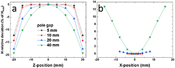
Figure 1. Magnetic field relative deviation (field uniformity) along the electromagnet axes: (a) Z-axis (X = 0, Y = 0) and b) X-axis (Y = 0, Z = 0) for different gaps from an electromagnet 3470 GMW associates with a circular pole face of 40 mm and 5 A current. Data courtesy of GMW associates from [5].
Download figure:
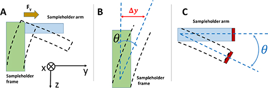
Standard image High-resolution imageIn this situation the presence of a paramagnetic SH can be problematic. As figure 2 shows, if a paramagnetic SH is placed in an inhomogeneous magnetic field (or misaligned), upon application of a field it will be magnetized, and a force will appear pushing the SH towards larger fields region in order to reduce Zeeman energy. Figure 2 illustrates this situation for a misalignment in x- and z-axis (figures 2(a)–(d) respectively). As the SH is fixed, these forces will arise a torque bending it. The effect is even (figures 2(a) and (b)) as it is showed in the appendix. In the case of misalignment in both, x and z directions, the dominant effect will depend on the geometry of the experimental set-up. Also, if the SH is perfectly centered and symmetric, the net force will be zero in the x- and z-directions, but not in the y-direction.
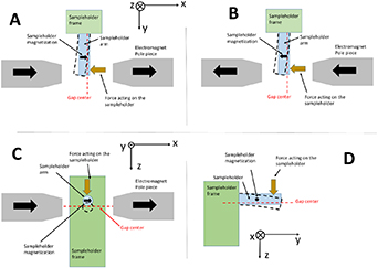
Figure 2. (a), (b) Scheme of magnetic field, magnetization and force on the SH upon application of a magnetic field with both orientations when the SH is misaligned in the x-axis. (c), (d) Zenital and axial views of field, magnetization and force when a SH is misaligned in the z-axis. Black dashed lines represent how the SH is displaced due to the forces acting on it.
Download figure:
Standard image High-resolution imageAs above indicated, the effect is even (it depends on the square of the magnetic field) and it will bend the SH in the same direction irrespective of the sense of the magnetic field applied in the x-direction. The larger the applied field, the larger the magnetization of the SH and consequently the torque acting on it.
Certainly, if the SH is perfectly centered and symmetric, the net force will be zero in the x-direction, but a small deviation will be enough to induce a net lateral force on the SH For some configurations, as polar MOKE, a symmetric disposition of the SH with respect to the magnetic field cannot be easily achieved, so a net force will be exerted on it. The force, and hence the deflection of the SH, will increase with the susceptibility (χ) of the SH material. Because the Zeeman Energy and therefore the force is proportional to susceptibility, an increase of one order of magnitude in χ will give rise to an appreciable increase in the torque acting on the SH When considering a MOKE setup, this force will shift the reflected spot onto the detector. This shift will increase with the applied magnetic field, depending on the susceptibility of the material used for the SH and on the configuration and dimensions of the SH [6]. If the reflected beam passes through a collimator, lens or it has a halo, this shift can lead to variation in the signal detected by the photodiode that will depend on the applied field.
3. Experimental artifact assessment
To illustrate the effect, figure 3 shows a MOKE magnetization curve for an aluminum film (for which no MOKE signal is expected) in polar configuration using a 303 annealed magnetic steel SH with susceptibility χ = 2·10−3. The above described symmetrical signal is clearly observed in the magnetization curve.
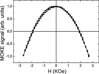
Figure 3. Polar MOKE magnetization curve for an Al film measured with a paramagnetic sample holder.
Download figure:
Standard image High-resolution imageIn order to analyze the effect when measuring ferromagnetic samples, we subsequently measured polar MOKE curves from a [Co (0.3 nm)/Pd (0.6 nm)] ([Co/Pd]) multilayer (with perpendicular anisotropy) using both, a paramagnetic (303 annealed steel, χ = 2·10−3) and a diamagnetic (PTFE, χ = − 1·10−5) SH Measurements were collected using a 635 nm solid-state laser beam in p-polarization at an incidence angle about 40 degrees. The beam was mechanically chopped at 107 Hz and the signal analyzed using a lock-in amplifier (SRS830 Stanford Research Systems) synchronized with the light modulator. Magnetic field was applied using an electromagnet (3470 GMW Associates) with 20 mm pole face.
Results are presented in figure 4. For the Teflon SH, a clear hysteresis loop characteristic of [Co/Pd] multilayers with perpendicular anisotropy (see figure 4(a)) is observed. On the contrary, when using the paramagnetic SH (figure 4(b)), the curve is a mixture of a symmetrical signal (as that showed in figure 3) plus an asymmetric contribution due to the real hysteresis loop of the sample. In this case, the symmetrical artifact is fairly larger than the real magnetization curve which makes the measurement not reliable for the analysis of the magnetic properties of the film. It should be noted that using paramagnetic materials with very low susceptibilities (of the order of 10–5) for the SH may avoid the effect caused by the SH deflection and, therefore, this artifact. Thus, an appropriate selection of the construction materials and a proper design of the SH are key factors to be considered when the MOKE experimental setup is conceived [7–10].
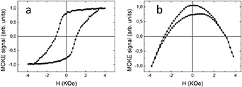
Figure 4. Polar MOKE curve for a [Co/Pd] multilayered film measured using (a) a diamagnetic SH and (b) a paramagnetic SH with very high magnetic susceptibility.
Download figure:
Standard image High-resolution imageNevertheless, measurements performed with paramagnetic SH exhibiting the above described artifact can be corrected to obtain the real hysteresis loops if certain conditions are fulfilled.
In particular, if the real magnetization curve is symmetric with respect to the origin, the proper curve can be recovered. This requirement of symmetry implies that no exchange bias, minor loops or any other effect inducing shifts of the curve are present.
4. Artifact removal procedure
To perform the correction we must divide the magnetization curve in four segments, named S1, S2, S3 and S4 that corresponds to: S1 from H = Hmax to H = 0; S2 from H = 0 to H = -Hmax; S3 from H = -Hmax to 0 and S4 from H = 0 to H = Hmax, as sketched in figure 5.
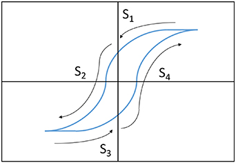
Figure 5. Scheme of the four segments a MOKE measurement in a normal magnetization cycle.
Download figure:
Standard image High-resolution imageEach of these signals Si, will have two contributions that we can name, the real signal Ri, coming from the sample, and the artifact Ai, given by the sample holder; that is, Si = Ri + Ai. If the real signal is symmetric, it turns out that


On the contrary, as the artifact signal is even, it comes out that

Now, subtracting:
So, the full curve can be recovered. To illustrate the validity of the procedure we have applied it to the curve presented in figure 4(b). Figure 6 compare the obtained curve with that measured with a Teflon SH Both curves match (despite some spikes due to experimental errors) demonstrating the validity of the processes to recover curves free of the described artifact.
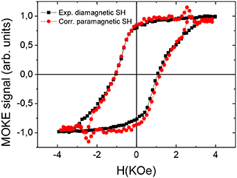
Figure 6. Magnetization curve measured with a paramagnetic SH and corrected as above described and the experimental curve measured with a diamagnetic SH.
Download figure:
Standard image High-resolution image5. Estimation of the sample holder bending and its influence on the MOKE signal
It is possible to perform an estimation of the dominant magnetic forces on the SH (see appendix for a detailed calculation). The exact force calculation is difficult and unfeasible for practical reasons, since it would require measuring the magnetic field in the volume of the SH arm. A practical calculation could be carried out by partitioning the SH arm in sections in which the field does not vary significantly. Thus, the applied magnetic induction field  can be replaced by a section average value
  and the integrals replaced by a sum over these sections (see Appendix).
To give some values to the discussion, we will consider a SH of square section wiBz≪By≲Bx
th lateral length of 7 mm (figure A1). Regarding the symmetry of the cylindrical poles of the electromagnet, it is expected that  inside the volume occupied by the SH arm and near the center of the gap. Please, notice the condition
  could be accomplished only outside the gap center as it could be the case of polar MOKE, where the SH arm is placed closer to one of the pole pieces. The main conclusion of these calculations (see details in the appendix) is that the y-component of the magnetic force is dominant in most situations. The x-component, second in order of relevance, could also be present.

Figure A1. Axial sketch in the yz plane of the sample holder described in this paper, showing the levers causing magnetic torques and their lengths.
Download figure:
Standard image High-resolution imageWe have performed numerical calculations to quantify these forces considering an square SH with a lateral cross section of 7 mm, a  at the center of the gap and a
  (303 annealed magnetic steel), obtaining
  . This force is pulling the SH arm from the upper end of the SH frame (see figure A2). With these values, further estimations could be performed to calculate the bending of the SH and the laser spot deflection. For instance, considering a Young modulus for the SH frame
  [11], and a SH frame length
  (figure A1), the area moment of inertia (see [11]) of the SH frame is
  , which result in a bending of
Figure A2. Bending of the sample holder (SH) frame due to y-component of the magnetic force; bending  of the SH frame and the displacement angle in (b) SH frame and (c) SH arm and sample.
Download figure:
Standard image High-resolution image
and a deflection angle of:  . This small deflection could be enough to cause a measurable effect in the Kerr signal, because is comparable to polarization changes in up to date MOKE setups (better than
  in Kerr rotation and changes of about
  in reflectivity [12]). Moreover, Kerr angles about
  in some films are not unusual [1]. If the setup disposes with a set of lenses to minimize the spot size (in some cases on the order of microns) it will imply spot displacements of the same order of the spot size. In addition, the reflected spot displacement will impinge on different positions of the photodiode, causing signal variations. This effect is not negligible even in the best case as described here and could be even more pronounced in cases where the SH is placed far from the center of the gap (as in some polar MOKE setups). On the contrary, for an analogous Teflon SH arm (
 we obtain
  ,
,  , and
, and  . Then, the effect caused remains below the MOKE sensitivity limit.
6. Conclusions
In summary, the use of paramagnetic sample holders in magneto-optical measurements can induce mechanical forces shifting the reflected beam and potentially modifying the intensity collected by the detector. This effect induces even spurious signals in the experimental magnetization curves that can be removed with a proper data treatment for symmetrical hysteresis loops. However, when possible, the use of diamagnetic or paramagnetic materials with low susceptibility (such as aluminum, bronze, etc) should be prioritized as suitable sample holder materials to avoid this artifact and therefore additional data processing.
Acknowledgments
This work was supported by the Spanish Ministry of Innovation, Science and Technology and Spanish Ministry of Economy and Competitiveness through Research Project MAT2017-86450-C4-1-R by the Regional Government of Madrid through Projects S2013/MIT-2850 (NANOFRONTMAG). A. M.-N. thanks Comunidad de Madrid and Universidad Complutense de Madrid for the project 2018-T1/IND-10360 granted by 'Atracción de Talento' program and The European Union for the H2020 research and innovation Marie Sklodowska-Curie Grant Agreement MAGNAMED 734801 (H2020-MSCA-RISE-2016). Drs. C. J. Bonin and F. Bonetto were reviewers on the original manuscript, the authors felt their contribution warranted authorship. Drs. C. J. Bonin and F. Bonetto were not used as reviewers on any revisions of the manuscript after they joined the authorship team. C. J. B. and F. B. acknowledge to CONICET for financial support.
Appendix A.: Detailed calculation of the magnetic forces on the sample holder
The magnetic force on a magnetic moment  at position
  is:
is:

where the Zeeman energy,  . For a small volume ΔV in the material the energy will be:
The magnetization  (being an average) is uniform and constant in ΔV and
  is the magnetic induction generated by the electromagnet at the center of ΔV. The magnetic permeability of the vacuum µ0 = 4π × 10 ―7 (H m−1) in SI units. Thus, we have:
Where  is the material volume magnetic susceptibility. The square of the applied magnetic induction is
  , showing explicitly that each component could vary from point to point. Then, and considering that the volume ΔV is the same throughout the material, the force on a small volume ΔV is obtained:

The components α = (x,y,z) of this force are, explicitly:
Note that we could approximate  and, consequently
  . Thus, obtaining the expression:
with β ≠ γ ≠ α. The α component of the total force on the material will be obtained by integrating in the volume V of the material:
Explicitly (see figure A1): if α = x, then [ ] and β = y and γ = z; if α = y, [
 ] and β = x and γ = z; and for α = z, [
 ], β = x and γ = y. Double integrals in equations runs on the respective sections of the SH arm (and may be the SH frame too).
The exact force calculation is difficult and unfeasible for practical reasons, since it would require measuring the magnetic field in the volume of the SH arm (and may be in the SH frame too). A practical and useful calculation could be carried out by partitioning the SH arm in sections in which the field does not vary appreciably. Then, the spatial variating magnetic induction  can be replaced by a section average value
  , and the integrals replaced by a sum over these sections:
And subsequently, the other components can be calculated:
Where, for example,  means average over the small area ΔyΔz along y-axis at the position x = xB;
  means average over the area ΔxΔz at the position y = yB;
 means average over the area ΔxΔy along y-axis and at the position z = zB; and so on.
It should be noted that, in all the cases, forces depend on the difference between square of the magnetic fields showing that the sense of forces does not depend on the sense of the current driving the electromagnet (consequently, the magnetic field sense). This fact is consistent with the parity of the experimental artifact observed as shown in figure 3. The sense of the force is towards higher(lower) field regions for paramagnetic (dia-) materials.
Further approximations could be made to simplify the estimation of the forces acting on the SH arm. If the cross section lengths are  and
and  , and considering the symmetry of the cylindrical poles of the electromagnet, it is expected that Bz < < By ≲ Bx inside the volume occupied by the SH arm in the setup showed in figure 2 (and near the center of the gap). The condition
  could be accomplished only outside the center of the gap as an extreme setup case or in other configurations (as in polar MOKE, for example when the SH arm is close to one of the pole pieces). Then the components of the force approximately are:
xB and xA, zB and zA are symmetric around x = z = 0 (center of the gap). Also,  and
and  throughout all the partitions of the SH arm (due to
  ) along y-axis; giving Fz ≈ 0.
Inspecting Fy force, one could also expect that  (at the position yA where the SH arm is fixed to the SH frame) but
  would be maximum (∼400mT from figure 4) at the position yB near the center of the gap, and that
  giving
On the other hand, by inspecting  force, one could also expect that
  and
and  (along the total length of the arm) if the SH is positioned near the center of the gap. In this way,
  .
.
Notice that the described situation is optimal because minimizes two of the three components of the magnetic force. The force parallel to the SH arm (y-axis here) is always present. If the SH arm is placed further from the center of the gap, the other components could not be negligible. From this, the y-component of the magnetic force would be the dominant and secondly the x-component of the force for this setup.