


Abstract
Conventional methods for the calibration of angle encoders typically only consider the graduation error of the encoder's circular scale. However, the radial motion of the circular scale during its rotation, due to its eccentricity and the axis of rotation radial error motion, can also introduce noticeable errors to the angle measurement in most practical applications. Based on the analysis of the influence of radial motion, an optimal-arrangement-based four-scanning-heads error separation technique for in situ self-calibration of angle encoders is presented. This Fourier-based technique uses the basic self-calibration model to measure the first-order Fourier component of the encoder error which includes the contribution of eccentricity. Meanwhile, the separation technique is utilized to separate the residual Fourier components of the graduation error from the measurement deviation due to radial error motion. The effect of the scanning heads' angular position errors on the calibration results is discussed. Optimal arrangements of the four heads are achieved to avoid the suppression of the Fourier components, and reduce the propagation of errors. Numerical results and experimental comparisons demonstrate the effectiveness of the proposed method. Moreover, this technique can also be used for measuring the spindle radial error motion for some users.
Export citation and abstract BibTeX RIS
1. Introduction
Angle encoders are widely used in applications that require angle measurement with high precision and high repeatability, such as rotary tables on machine tools, positioning systems and angle comparators [1–4]. During the angle measuring process, the accuracy is inevitably influenced by the error of angle encoder. Errors of the angle encoder can generally be classified into two categories: the encoder-specific error, and the application-dependent error. The former includes graduation error of the encoder's circular scale due to manufacture and mounting, and interpolation error which becomes apparent in very small angular scales. The latter is mainly caused by the radial motion (also known as lateral shift) of the circular scale (including its eccentricity and the radial error motion of the measured spindle), and the alignment of scanning head [2, 4]. In practical applications, calibration is necessary to determine and further eliminate the encoder error [1].
Generally, based on the subdivision of the full circle and the principle of circle closure [5], two types of calibration techniques are available for calibrating angle encoders, i.e. cross- and self-calibration methods. Cross-calibration method requires a second measuring device, and compares the angles of the encoder to be calibrated with those of the second device. It can determine the errors of both the encoder and the second device [1, 6]. However, the involving measuring process is time-consuming, and the number of calibration angles is limited. By using reversal, redundancy and error separation techniques, various self-calibration methods have been developed for accurate measurement of part features in dimensional metrology, without reference to any externally calibrated artefacts [7]. A number of efficient methods have also been proposed for the self-calibration of angle encoders, such as the equal division averaged (EDA) method [8–13], the time-measurement dynamic reversal (TDR) method [3], the prime factor division (PFD) method [14] and the Fourier method [15]. These methods have the advantage of fast in situ calibration, and most of them rely on special arrangements of multiple scanning heads at different angular positions. The Fourier approach, proposed by Geckeler et al [15], is ideally suited for calibration of encoders, since it does not depend on specific arrangement of scanning heads and can be applied universally. By using the Fourier method, the optimal arrangement schemes of two and three scanning heads are obtained in the previous work [16], achieving the same calibration performance but with fewer heads, compared to the regular arrangements.
The above methods usually only focus on the circular scale's graduation error, since the application-dependent error is much smaller than the graduation error in high precision calibration systems (e.g. in National Metrology Institutes). However, in many industrial applications, due to the radial and tilt error motions of the axis of rotation, the radial motion of the encoder's circular scale relative to its scanning head has noticeable effect on the angular positioning error of the rotary table [17]. In these cases, it is inadequate just to evaluate the graduation error, and the above calibration methods will be inaccurate since the application-dependent error is neglected. Therefore, both errors should be included in the calibration analysis, even in high precision systems. Several works have been presented to solve this problem. In [18], an improved TDR method is proposed, with considering the influence of spindle radial error motion. At the Physikalisch-Technische Bundesanstalt (PTB), an extended self-calibration model has also been introduced to improve the estimation of the graduation error [19, 20]. Compared to their earlier work [15], the new extended model in [19] can evaluate and correct the error influences due to radial motions of the circular scale. By using an iterative approach, a more accurate estimate of the graduation error can be obtained and the radial motion of the circular scale can also be determined. The iterative approach is feasible when the magnitude of the influence of radial motion on the head's angle measurements is very small compared to the influence of the graduation error (in the case of the PTB's high-precision angle comparator WMT 220, two orders of magnitude). So far, a direct (without iteration) and universal error separation technique to separate the graduation error from the error due to radial motion has been little discussed.
Since the encoder error is associated with the geometric accuracy of axis of rotation, it is natural to compare the encoder calibration methods with the spindle metrology techniques. In fact, as the two most commonly used spindle error motion separation techniques, the multistep method uses the same principle as the EDA method [10, 21], and the multiprobe method is also based on the Fourier analysis [22–25]. In addition, the relation between the graduation error of circular scale and the angle deviation due to its radial motion is very similar to the relationship between the artefact form error (out-of-roundness) and the radial error motion in spindle metrology [26]. Therefore, it is expected that the error separation for encoder calibration can also be realized by using multiple scanning heads, just like the multiprobe method.
Based on the basic Fourier method of encoder calibration [15, 19] and the foundation of spindle error motion measurement, this paper presents an error separation technique for calibrating the angle encoder. The influence of circular scale's radial motion on scanning head's angle measurement is analyzed in detail. The four-scanning-heads method is then proposed for separating the graduation error of circular scale from the error caused by its radial motion. The effect of heads' angular position errors on the separation results is discussed. Furthermore, by using a similar optimization approach presented in [16], optimal arrangements of the four heads are determined to reduce harmonic suppression. Simulations and experiments are performed to validate the method. This method provides a useful and accurate solution for self-calibration of angle encoders in practical measurement tasks.
2. Background
2.1. Basic angle encoder self-calibration method
The basic Fourier-based angle encoder self-calibration method using multiple scanning heads [15, 19] is briefly reviewed in this section. Figure 1 shows an arrangement of the heads (at least two heads can be used for calibration in the basic method; at least four heads as shown in figure 1 are required in error separation model, which will be discussed in section 3.2). During the rotation of circular scale, in addition to the rotation angle θ, the angles measured by the head Hk are also influenced by the circular scale's graduation error ε(θ), including a phase shift due to the head location (α1 = 0), as shown in equation (1) (assuming rotating the scale in a clockwise direction),

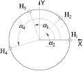
Figure 1. Schematic of the multiple scanning heads method.
Download figure:
Standard image High-resolution imageIn order to eliminate the unknown rotation angle θ, the angle difference δkr(θ) between any two simultaneously measured data can be applied

Due to the periodic nature of the graduation error, Fourier analysis shall be a powerful tool for evaluating the obtained data. By using the discrete Fourier transform (DFT), equation (2) can be written as

where Ekr(n) and F(n) are the Fourier coefficients of δkr(θ) and ε(θ), respectively, n is the Fourier order and Wkr(n) is the transfer function from F(n) to Ekr(n). Given Ekr(n) and Wkr(n), the graduation error can be derived by applying the inverse discrete Fourier transform (IDFT)
In some applications, three or more heads are used to improve the accuracy of the calibration result. In these cases, the Fourier coefficients F(n) can be derived from a weighted combination of the measurement differences by all pairs of scanning heads
where the normalized weights pkr(n) in equation (6) can be chosen [19], which can provide the minimal error propagation with respect to the Fourier coefficients F(n)
The basic self-calibration method may be sufficient for applications in which the graduation error is dominant compared with other error influences, especially for high-precision angle comparators. However, in the general application of angle encoder, the radial motion of the encoder's circular scale during its rotation, including its eccentricity relative to the spindle which carries it, and the radial error motion of the spindle rotor, is usually another important factor that influences the angle measurements by the scanning heads [19]. It is thus necessary to evaluate and separate the effect of the circular scale's radial motion by using an error separation technique, as will be discussed in section 3. For a better understanding of the whole principle, background of the spindle error motion, as well as its measurement using the multiprobe method, is reviewed in section 2.2.
2.2. Spindle radial error motion and multiprobe error separation
According to ISO 230-7 [27], spindle error motions are unwanted changes in position and orientation of the axis of rotation relative to its axis average line as a function of rotary position of the rotor. Error motions can be directionally decomposed into axial error motion (along Z axis), pure radial error motion in X and Y directions, and tilt error motion around X and Y axes. In practice, pure radial error motion and tilt error motion occur at the same time, and the sum at any specified axial location is defined as radial error motion. Axial error motion has no influence on angle measurement by scanning head. Radial error motion at the axial position where the circular scale locates can influence the head's angle measurement. Error motion can also be divided into synchronous and asynchronous components based on rotational frequency. The synchronous error motion is the repeatable component of the total error motion calculated by averaging the data from the number of revolutions and it consists of Fourier components that occur at integer multiples of the rotation frequency. The asynchronous (non-repeatable) component is the deviations of the total error motion from the synchronous and it may contribute to the repeatability of the encoder calibration results during repeat measurements. Therefore, this paper focuses on the synchronous radial error motion.
In general, the spindle error motion can be measured with a capacitive displacement sensor targeting a cylindrical or spherical test artefact. However, for the 2D radial error motion, error motion values measured with sensors at different fixed radial sensitive directions may vary greatly. Here, the term 'sensitive direction' in spindle metrology represents direction perpendicular to the workpiece surface through the point of measurement. Fortunately, the radial error motion for a fixed sensitive direction at an angle βk with respect to X axis (see figure 2), can be calculated using equation (7).

where, x(θ) and y(θ) are components of the radial error motion in X and Y directions, respectively.
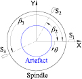
Figure 2. The multiprobe method for spindle radial error motion separation.
Download figure:
Standard image High-resolution imageMeasurement of spindle radial error motion is influenced by the roundness error of the artefact against which the sensor senses. For highly accurate measurements, the radial error motion should be separated from the artefact roundness error using error separation techniques. One of the most commonly used separation techniques is the multiprobe method, which uses three or more sensors to simultaneously measure the combination of the error motion and roundness error, as illustrated in figure 2. The measurements of the three displacement sensors S1, S2 and S3, are a summation of the X and Y components of the radial error motion, and the artefact roundness error r(θ), with a phase shift due to the sensor location,
A weighted combination of these three measurements, S(θ), can be used to remove the contribution of radial error motion

where the unknown coefficients b1, b2 and b3 should satisfy
By solving equation (10), the following relationship is obtained

For convenience, b1 = sin (β3 − β2), b2 = −sin β3 and b3 = sin β2 can be defined.
Then, equation (9) contains only the information about the roundness error. Applying the DFT to equation (9) gives

where B(n) is the transfer function from r(n) to S(n). When the coefficients S(n) and B(n) are known, the artefact roundness error can be determined by using the IDFT

By substituting r(θ) in equation (8), the X and Y components of the radial error motion can be calculated

3. Error separation technique for angle encoder calibration
3.1. Angle deviation caused by radial motion of circular scale
The basic self-calibration method in section 2.1 considers the graduation error only. However, the angle encoder error is also influenced by the circular scale's radial motion. The influence of radial motion on head's angle measurement has been analyzed in [19]. This section recapitulates the main theoretical analysis, and, at the same time, gives more details about the measurement deviations of the heads due to 2D radial error motion. Figure 3 shows how the radial motion of circular scale affects the angle measurement by scanning head. Ideally, during the rotation of the circular scale, its radial center should always coincide with the geometric center of the fixed arrangement of scanning heads (i.e. the spindle stator center, the origin of the coordinate system, O). In practical applications, however, due to the mounting eccentricity and the spindle radial error motion, the circular scale center will have a radial motion from O(0, 0) to O' (x, y). This results in a deviation between the angle θ' detected by the head Hk (located at angle αk with respect to X axis) and the real rotation angle θ (assuming a clockwise rotation). Since the deviation, λk(θ) = θ' − θ, is very small (usually, <0.01°), it can be approximated as

where R is the circular scale radius (mean graduation radius), and h can be calculated according to

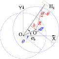
Figure 3. Influence of circular scale's radial motion on scanning head's angle measurement.
Download figure:
Standard image High-resolution imageThus, the heads' measurement deviations due to radial motion of the circular scale during its rotation are a function of the circular scale radius, the radial motion and the heads' position angles, and can then be represented as [19]
As a quantitative evaluation, figure 4 presents the peak-to-valley (pv) magnitude of the measurement deviation as a function of the circular scale radius, with the ranges of radial motion, max(h(θ)) − min(h(θ)), being equal to 0.02 µm, 0.05 µm, 0.1 µm, 0.2 µm, 0.5 µm, and 1 µm, respectively. The influence of the radial motion can be reduced by using a circular scale with larger radius. It should be noted that, however, when the range of radial motion is 0.1 µm, the magnitude of angle deviation is greater than 0.1 arcsec, even for a large radius R = 180 mm. Hence, the influence of the circular scale's radial motion cannot be simply neglected for high-precision measuring tasks.
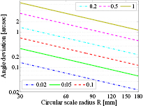
Figure 4. Angle deviation for different ranges of radial motion as a function of circular scale radius.
Download figure:
Standard image High-resolution imageNote that for angle measurement, averaging the measurement values of the scanning heads which are arranged at regular intervals can eliminate the effect of circular scale's radial motion. This can be explained by the following mathematical property
Therefore, for M equally distributed heads with position angles αk = 2π (k − 1)/M, the sum of their measurement deviations (see equation (17)) due to radial motion satisfies
In particular, for industrial application of angle encoders, a common method of eliminating the influence of radial motion is to mount two scanning heads at 180° angular interval.
The mounting eccentricity of the circular scale relative to the spindle is one of the two physical causes of radial motion [19]. For the eccentricity e (i.e. the offset |OO'| = e, see figure 3), assuming that the eccentricity vector has an angle θe with respect to the X axis at rotation angle θ = 0°, h(θ) in equation (16) will be equal to e sin(αk − θe + θ). Then, equation (17) can be written as
By comparing this equation with the graduation error ε (θ + αk) shown in equation (1), it can be found that the angle deviation caused by the eccentricity automatically conforms to the graduation error model. The basic self-calibration method can correctly evaluate the influence of eccentricity as the first-order Fourier component of the encoder error. Therefore, the eccentricity should not be treated as a source of additional error influence (relative to the graduation error), since its influence completely conforms to the basic self-calibration model [19].
The spindle radial error motion is another cause of radial motion. In fact, the eccentricity error is the first-order Fourier component of the radial motion, while the radial error motion contributes to the residual components of radial motion in the frequency domain. In order to demonstrate the influence, and further separation approach, of the radial error motion, figure 5 provides a numerical simulation example used throughout section 3: the spindle 2D radial error motion in X and Y directions, and the circular scale's graduation error (including the first-order Fourier component caused by eccentricity).
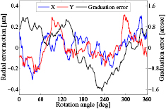
Figure 5. A numerical example of the spindle 2D radial error motion in X and Y directions and the circular scale's graduation error.
Download figure:
Standard image High-resolution imageThe measurement deviations of the scanning heads caused by the 2D radial error motion can be calculated by equation (17), as shown in figure 6, for the heads' angular positions αk = 0°, 40°, 90° and 180°, respectively (the circular scale radius is assumed to be 150 mm). The deviations of the heads at 0° and 180° orientation angles show equal magnitudes but opposite signs, as mentioned in equation (19) (M = 2). In addition, equation (17) can also be expressed as λk(θ) = (x(θ) cos(αk − 90°) + y(θ) sin(αk − 90°))/R. By comparing this expression with equation (7), the 90° angular difference in phase reveals an important relation between angle encoder calibration and spindle metrology. For a direction where the sensor (scanning head or displacement sensor) is fixed, the displacement sensor is sensitive to the component of the 2D radial error motion along the fixed direction (radial measurement), while the head is sensitive to the component of the radial motion perpendicular to this direction (tangential measurement), see section 2.2 and figure 3. Therefore, it should be noted that the meaning of 'sensitive direction' is different for spindle metrology and encoder calibration. For this reason, the head's deviation at 90° angular position in figure 6 and the X component of the radial error motion in figure 5 have the same curve shape, and so do the deviation at 180° and the error motion in Y direction. (Note that the clockwise rotation of circular scale is assumed in this paper; for anticlockwise rotation, equation (17) will be opposite in sign).
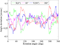
Figure 6. Measurement deviations of the scanning heads at different position angles, due to the 2D radial error motion of the numerical example.
Download figure:
Standard image High-resolution imageFurthermore, the differences in heads' measurement deviations due to the 2D radial error motion at different position angles are substantial. In figure 6, the pv range of the angle deviation at 40° angular position is obviously less than the other three ranges. Figure 7 plots the pv range of the measurement deviation, max(λ(θ)) − min(λ(θ)), as a function of the head's angular position αk. Since measurement deviations for two heads separated by 180° are opposite in sign, the plot has a period of 180°. In this numerical example, the range of measurement deviation is substantially less at angular positions between 30° and 45° (or between 210° and 225°) than at other angular positions. Thus, for angle measuring tasks, these angular positions can be used as preferential measurement points to help reduce the influence of radial error motion.
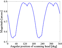
Figure 7. The pv ranges of measurement deviations at different heads' position angles, based on the influence of the 2D radial error motion in figure 5.
Download figure:
Standard image High-resolution image3.2. Four-scanning-heads error separation
In the basic self-calibration method, graduation error is the only factor that affects the angle measurement by scanning head. However, angle deviation caused by circular scale's radial motion is another important factor that influences the measurement. In this section, an error separation method is introduced for separating the graduation error from the angle deviation due to radial motion.
After introducing the measurement deviation λk(θ) shown in equation (17), the angles measured by the head Hk in equation (1) yield
Especially for the reference head H1, we have

Since there are four unknowns in equation (21), at least four heads should be used for the separation (see figure 1). Then, the angle differences for the heads H2, H3, and H4 relative to the reference head H1 can be obtained to eliminate the rotation angle θ,

In order to remove the influence of the 2D radial motion, a weighted summation of these angle differences can be used
where the unknown coefficients a1, a2 and a3 should satisfy
Solving equation (25) gives
where C is an arbitrary constant. For convenience, C = 1 is used in this paper.
After removing the contribution of radial motion and by applying the DFT, equation (24) can be expressed as E(n) = W(n)F(n). The transfer function W(n) is represented as

Then the graduation error ε(θ) can be obtained by using the IDFT, just like equation (4).
In addition, the radial motion components x(θ) and y(θ) can be calculated by substituting the graduation error ε(θ) in equation (23),
with
This separation process, however, cannot separate the first-order Fourier component, since the transfer function W(1) is always equal to 0 no matter what the position angles α2, α3 and α4 are set. Nevertheless, as stated in section 3.1, since measurement deviations due to the eccentricity, i.e. the first-order component of radial motion, conform to the graduation error model, the first-order component of encoder error can be well obtained by using the basic self-calibration method. As a result, the whole calibration process, simulated with the numerical example in figure 5, is illustrated in figure 8 (assuming α2 = 60°, α3 = 135° and α4 = 228° in this simulation; the reason for selecting these position angles will be discussed in section 4).
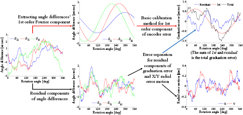
Figure 8. The whole calibration process. The first-order Fourier component of the encoder error is calibrated by using basic self-calibration method, while the residual graduation error and the X and Y components of radial error motion are obtained by applying the four-scanning-heads error separation technique.
Download figure:
Standard image High-resolution imageIt is important to note that the 2D radial error motion can also be determined from the four-scanning-heads error separation method. Therefore, this method may be an important tool for measuring the radial error motion in practical applications.
3.3. Influence of scanning heads' angular position errors
The multiple scanning heads methods for calibration of angle encoders require exact mounting and adjustment of the heads. In practice, the scanning heads' angular position errors, i.e. the deviations between the actual angular positions and their nominal values, are inevitable. At the PTB, the contribution of the uncertainty of heads' angular positions to the uncertainty of reconstructed graduation error was evaluated according to Monte Carlo approach [19]. In this section, the influence of the heads' angular position errors on the accuracy of self-calibration results is discussed based on theoretical and numerical analyses.
Taking the scanning head H1 in figure 1 as the reference head, and denoting the angular position error of head Hk relative to H1 as ηk, the angle measurement by Hk then deviates from the value Hk(θ) in equation (21), and can be expressed as
The measurement error on the angle difference δk1(θ) is given by
For the very small value of ηk, we have cos ηk ≈ 1, sin ηk ≈ ηk. Equation (31) can be rewritten as
For simplicity, only the position of head H2 is first assumed to have an angular error. Then the deviation on δ(θ) in equation (24) yields

Using the DFT, equation (33) becomes
The errors on the Fourier coefficients of ε(θ) yield ΔF(n) = F'(n) − F(n) = ΔE(n)/W(n), and can be further expressed as
Finally, for the measurement error on the graduation error, we have Δε(θ) = ε'(θ) − ε(θ) = IDFT(ΔF(n)).
Equation (35) reveals the effect of head's angular position error on the calibration result for the four-scanning-heads error separation method. When neglecting radial error motion (x = 0 and y = 0), this equation gives the measurement error for the basic method in section 2.1. From equation (35), the measurement error resulting from angular position error contains contributions of both the graduation error and the radial motion. The Fourier component ΔF(n) is a linear combination of the graduation error's component F(n) and the radial motion's components x(n) and y(n), but is inversely proportional to the transfer function W(n). However, it should be noted that the coefficient of F(n), exp(inα2) (exp(inη2) − 1), varies with Fourier order n, while the coefficient of [x(n)cosα2 + y(n)sinα2]/R remains constant (η2). Figure 9 gives the amplitude of the coefficient exp(inη2) − 1 as a function of the order n (|exp(inα2)| = 1), with the angular position error η2 = 120 arcsec, −240 arcsec and 360 arcsec, respectively. The linear relation between the amplitude and the order shows that high order Fourier components of the reconstructed graduation error are more susceptible to the head's angular position error, which conforms to the analysis in our previous publication [16]. Although low order components of the graduation error usually have larger amplitudes, their contribution to Δε(θ) is limited to a relatively higher degree.
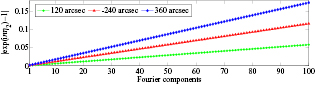
Figure 9. Variation of amplitude of the coefficient, exp(inη2) − 1, with the Fourier order n, at angular position error η2 = 120 arcsec, −240 arcsec and 360 arcsec, respectively.
Download figure:
Standard image High-resolution imageIn addition, for the order n = 1, we have |exp(iη2) − 1| = |η2| (i.e. |η2| = min(|exp(inη2) − 1|), n integer and ≠ 0). From this equation and equation (35), it can be seen that all the Fourier components of radial motion have the same influence coefficient on the corresponding components of the measurement error; moreover, the contribution of radial error motion to the measurement error is much less than that of graduation error. Figure 10 shows the measurement error on the reconstructed graduation error ε(θ) at the angular position error η2 = 360 arcsec, based on the numerical example shown in figure 5. As described above, low order components are inconspicuous in the measurement error. By assuming that the measured graduation error is not influenced by the angular position error (making ε (θ + α2 + η2) − ε (θ + α2) = 0, in equation (32)), the contribution of radial error motion to Δε(θ) is also presented in figure 10. It is negligibly small, compared to the total measurement error.
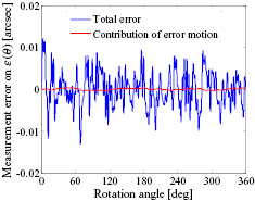
Figure 10. Measurement error on the reconstructed graduation error at angular position error η2 = 360 arcsec, for the numerical example in figure 5. The contribution of radial error motion is negligibly small, compared to the total measurement error.
Download figure:
Standard image High-resolution imageFigure 11 shows the magnitudes (pv range) of the measurement errors on graduation error, Δε(θ), and on radial error motion in X and Y directions, Δx(θ) and Δy(θ), respectively, when η2 ranging from 60 arcsec to 600 arcsec at 60 arcsec intervals. The measurement errors increase linearly with respect to the increasing angular position error. Since the radial error motion can be calculated only after the calculation of graduation error (see equation (28)), the measurement errors Δε(θ), Δx(θ) and Δy(θ) are correlated. The dominant contribution to measurement errors caused by scanning heads' angular position errors is the graduation error.
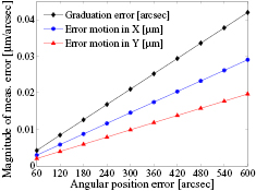
Figure 11. Magnitudes of the measurement errors on graduation error and radial error motion in X and Y directions, respectively, with angular position error η2 ranging from 60 arcsec to 600 arcsec, for the numerical example in figure 5.
Download figure:
Standard image High-resolution imageFinally, for the four-scanning-heads method, the expressions of ΔF(n) for the other two heads' angular position errors, η3 and η4, are similar to equation (35), except for their corresponding subscripts. The total measurement error of the four-scanning-heads system can be expressed as a linear superposition of the errors due to individual angular position errors.
4. Optimization of four scanning heads arrangement
In early work [16], based on the basic self-calibration method, the optimal arrangements for two and three scanning heads are obtained. In this section, the optimization of four heads arrangement is performed, since the calibration performance of the four-scanning-heads method is also highly dependent on the geometrical arrangement of heads. For a given arrangement, the transfer function W(n) in equation (27) may be equal to zero on some Fourier orders. This can result in an ineffective separation of the Fourier components of graduation error and spindle error motion on these orders (i.e. the phenomenon of harmonic suppression). Figure 12 gives the amplitude of W(n) for the first 50 Fourier orders for three different arrangements of the four heads. It can be seen that for the regular arrangement of the four heads (distributed at intervals of 90°) the Fourier components with orders n = 4j and 4j ± 1 (j integer) are suppressed. Similarly, for α2 = 72°, α3 = 144° and α4 = 216°, with the greatest common divisor (GCD) of the angles being 72° or 2π/5 radian, W(n) = 0 for orders n = 5j and 5j ± 1. For α2 = 30°, α3 = 60° and α4 = 150° (the GCD is 30° or 2π/12 radian), the components with orders n = 12j and 12j ± 1 are suppressed. This can be explained by equations (36) and (37).

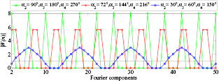
Figure 12. Transfer functions |W(n)| for three different arrangements of the four scanning heads. Harmonic suppression occurs for those Fourier components at which |W(n)| = 0.
Download figure:
Standard image High-resolution imageAssuming that the GCD of α2, α3, α4 and 2π is ϕ, and the ratios between these four angles and ϕ are d2, d3, d4 and D respectively, we have Dα2 = d22π, Dα3 = d32π and Dα4 = d42π. The following relationship can be obtained
Finally, combining the two equations yields W(n) = 0, for n = jD, jD ± 1.
In addition, if the transfer function W(n) is too close to zero, a small measurement error on E(n) due to uncertainty of the calibration system will cause a relatively large error on F(n) [16]. Therefore, it is necessary to find the optimal arrangements to avoid harmonic suppression and to reduce the propagation of measurement error.
In this paper, the optimization goal is to determine the most appropriate arrangements for angles α2, α3 and α4 to maximize the minimum value of the transfer function |W(n)| for the first N orders (except the 1st order). N = 100 is chosen in this work, since the first 100 Fourier components will suffice for most applications in industry. As a matter of convenience, we define ϕ1 = α2, ϕ2 = α3 − α2 and ϕ3 = α4 − α3 as the objective function's variables during the optimization process.
To avoid repeated solutions and reduce computational time, boundary constraints need to be appropriately determined. Theoretically, for four angular intervals (see figure 13), there are 24 (4!) permutations. However, as shown in figure 13, only three arrangement schemes are independent, because each scheme has 8 permutations (every angular interval can be used as the first one; 4 permutations in anticlockwise direction, 4 permutations in clockwise direction), and transfer functions |W(n)| for the 8 permutations in each scheme are identical. In order to use this condition in the calculation process, the following constraints can be made: ϕ1 ⩽ ϕ2, ϕ1 ⩽ ϕ3, ϕ1 ⩽ ϕ4 and ϕ2 ⩽ ϕ4 (ϕ4 = 360° − ϕ1 − ϕ2 − ϕ3).
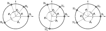
Figure 13. Three arrangement schemes of the four heads at a given set of angular intervals.
Download figure:
Standard image High-resolution imageFinally, the 3D optimization problem can be formulated as
- maximize min |W(n)| n = 2, ..., N
- subject to 10° ⩽ ϕ1 ⩽ 90°
- ϕ1 ⩽ ϕ3 ⩽ 360° − 3ϕ1
- ϕ1 ⩽ ϕ2 ⩽ 180° − (ϕ1 + ϕ3)/2.
Here, the lower bound 10° is chosen for the consideration of the limit by geometric size of the scanning heads.
A convenient way to solve this 3D problem is to show the minimum value of |W(n)| from the 2nd to Nth Fourier order for all combinations of angles α2 (ϕ1), α3 − α2 (ϕ2) and α4 − α3 (ϕ3) in a specific step size. As an example, figure 14 gives the distribution of the min |W(n)| for angles α4 − α3 and α3 − α2 at α2 = 60° in a step size of 0.1° (N = 100). It can be seen that this objective function is highly nonlinear, non-convex and has many local optima. The blue regions represent the bad solutions where harmonic suppression and/or amplification of measurement error will occur. Red regions, especially those with (min |W(n)|) > 1, mean the preferred angle combinations, since no Fourier component is suppressed and the error propagation is reduced.
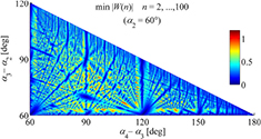
Figure 14. Distribution of the minimum value of |W(n)| for angles α4 − α3 and α3 − α2 at α2 = 60° (N = 100). This objective function is highly nonlinear, non-convex and contains multiple local maxima.
Download figure:
Standard image High-resolution imageIn practical applications, arrangements for angles with integer degrees are easier to use. Therefore, this paper mainly focuses on the integer optimal solutions. The global integer optimum is α2 = 60°, α3 = 135° and α4 = 228°. The values of |W(n)| for this arrangement is shown in figure 15. In this case, all the amplitudes of W(n) are larger than 1 (the minimal value is |W(n)| = 1.1763, at Fourier orders n = 42 and 78).
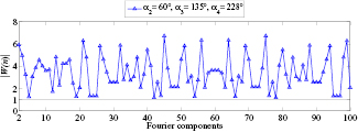
Figure 15. Transfer functions |W(n)| for the global integer optimal arrangement.
Download figure:
Standard image High-resolution imageObviously, other integer solutions, with (min |W(n)|) > 1 (N = 100), are also appropriate choices for the actual use of angle encoder. By our calculation, a total of 38 integer optimal solutions satisfy this condition, as listed in table 1.
Table 1. Integer optimal arrangements with min |W(n)| being larger than 1 (n = 2, ..., 100).
| α2 (deg) | α3 (deg) | α4 (deg) | |
|---|---|---|---|
| 1 | 36 | 117 | 210 |
| 2 | 36 | 120 | 225 |
| 3 | 39 | 120 | 213 |
| 4 | 40 | 110 | 233 |
| 5 | 42 | 102 | 243 |
| 6 | 45 | 108 | 192 |
| 7 | 51 | 117 | 231 |
| 8 | 53 | 112 | 233 |
| 9 | 54 | 144 | 249 |
| 10 | 54 | 144 | 267 |
| 11 | 55 | 120 | 237 |
| 12 | 56 | 126 | 241 |
| 13 | 57 | 144 | 219 |
| 14 | 57 | 132 | 234 |
| 15 | 57 | 132 | 240 |
| 16 | 57 | 135 | 252 |
| 17 | 59 | 134 | 262 |
| 18 | 60 | 135 | 228 |
| 19 | 60 | 129 | 237 |
| 20 | 61 | 168 | 232 |
| 21 | 61 | 160 | 247 |
| 22 | 61 | 128 | 241 |
| 23 | 63 | 141 | 231 |
| 24 | 63 | 147 | 245 |
| 25 | 65 | 133 | 279 |
| 26 | 67 | 170 | 251 |
| 27 | 67 | 137 | 226 |
| 28 | 67 | 137 | 262 |
| 29 | 68 | 153 | 224 |
| 30 | 69 | 150 | 237 |
| 31 | 69 | 168 | 255 |
| 32 | 69 | 162 | 257 |
| 33 | 69 | 159 | 267 |
| 34 | 69 | 141 | 273 |
| 35 | 71 | 148 | 249 |
| 36 | 73 | 149 | 243 |
| 37 | 73 | 149 | 249 |
| 38 | 75 | 156 | 260 |
5. Experiments
In this section, the error separation technique for self-calibration of angle encoder is validated. The global integer optimal arrangement presented in section 4 is adopted. Additionally, in order to verify the effectiveness of separation results, an attempt is made to compare the spindle radial error motions obtained from the four-scanning-heads approach and the multiprobe method (see section 2.2). To ensure that the two methods measure radial error motion at the same axial location, the three capacitive displacement sensors used in multiprobe method are also positioned radially against the encoder scale drum, as shown in figure 17(b). Figure 16 shows the arrangement of the four heads and the three capacitive sensors on the circumference of the scale drum. The first sensor S1 is arranged with interval −90° relative to the head H1 so that measured radial error motions can be conveniently compared. Measurement angles β2 = 55° and β3 = 113°, obtained by using a similar optimization method, can be used to avoid harmonic suppression and realize full separation from 2nd to 100th harmonic.
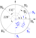
Figure 16. Arrangement of the four scanning heads and the three capacitive displacement sensors in the experiment.
Download figure:
Standard image High-resolution image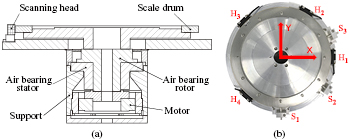
Figure 17. Experimental setup. (a) Schematic diagram of the rotary table, (b) photograph of the arrangement of scanning heads and capacitive sensors.
Download figure:
Standard image High-resolution imageFigure 17 shows the experimental calibration setup, an air-bearing rotary table fitted with an incremental angle encoder for high accuracy (Heidenhain ERA 4282 C) [4]. The encoder consists of a scale drum and four scanning heads. The scale drum has 52 000 signal periods corresponding to a signal period of about 24.92 arcsec, and its grating period is 20 µm corresponding to the drum outside diameter of 331.31 mm. Each signal period is then digitally interpolated with the factor 4096. Consequently, the resolution of the angle measuring system is about 0.006 arcsec. The scanning heads are mounted by strictly following the mounting instruction, and exactly aligned by performing fine adjustment. The capacitive sensors (Lion Precision C8-2.0) are located at the same axial location as the scanning head's sensing window. Moreover, capacitive sensor can also be used for precisely centering the scale drum. All the angular position errors of four heads and three capacitive sensors are adjusted within ±0.05°. A direct-drive, slotless, brushless motor is used to rotate the rotor. Note that the motor may have a significant influence on the axis of rotation radial error motion. The whole setup is mounted on an optical table which is isolated from external vibrations.
The measurement is made at a constant speed of 0.5 rpm. All signals of the four heads and the three capacitive sensors are collected synchronously by using ACS motion control system, and 24 000 measured data can be obtained in one revolution for each signal. The three measurements S1(θ), S2(θ) and S3(θ) and the three measured angle differences δ21(θ), δ31(θ) and δ41(θ) are then digitally filtered to 100 cycles per revolution for subsequent analyses. The effect of the asynchronous error motion is filtered out by averaging the data over 20 revolutions.
The calibration results using four scanning heads are presented in figures 18 and 19. Figure 18 shows the encoder error. The 1st order Fourier component of the encoder error, indicating the influence of eccentricity, is achieved by applying the basic self-calibration method in section 2.1. The residual graduation error (blue line in figure 18) and the 2D radial error motion in X and Y directions (figure 19) are obtained by the four-scanning-heads error separation method. The total encoder error (black line in figure 18) is a superposition of the 1st order error and the residual error. It can be seen that the 1st and 2nd harmonics are predominant components of the encoder error. The pv ranges of the radial error motion in X and Y directions are larger than 0.18 µm and 0.26 µm, respectively. The magnitude of angle deviation caused by the error motion will be greater than 0.1 arcsec, as demonstrated in figure 4. Therefore, for this experiment, the influence of the radial error motion should not be neglected.
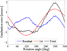
Figure 18. Graduation error of the angle encoder's scale drum of the rotary table. First-order component of the encoder error (red) is determined by basic self-calibration method, while residual graduation error (blue) is obtained based on four-scanning-heads error separation method. The total error (black) is a superposition of the two errors.
Download figure:
Standard image High-resolution image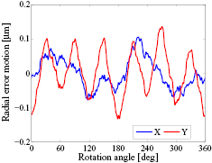
Figure 19. The synchronous radial error motion in X and Y directions measured by the four-scanning-heads error separation method.
Download figure:
Standard image High-resolution imageAs a validation, by applying basic self-calibration method, four calibration results of the graduation error, obtained by two heads H1 and H2 (calculated using the measurement difference δ21(θ)), H1 and H3 (δ31), H1 and H4 (δ41), and all four heads H1 to H4 (δ21, δ31 and δ41), are compared before and after removing the influence of radial error motion (values calculated from the error separation method, see figure 19) from each angle difference, as shown in figure 20. Figure 20(a) shows the four curves solved directly using the measured angle differences. Figure 20(b) presents the results using modified angle differences, where the deviations caused by radial error motion are removed (i.e. the last terms on the right-hand side of equation (23), [x(θ)sin αk − y(θ)(cos αk − 1)]/R). From both figures it is clearly seen that the differences between the four results, when the influences of radial error motion are corrected, are reduced substantially. Note that the remaining differences of the curves in figure 20(b) are mainly due to the harmonic suppression in two heads calibration results.
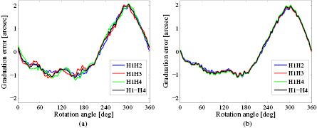
Figure 20. Calibration results based on basic self-calibration method by using different heads before (a) and after (b) removing the influences of radial error motion presented in figure 19.
Download figure:
Standard image High-resolution imageAs another tentative comparison, the radial error motion separation results using the multi-probe method are shown in figure 21. Compared with figure 19, the essential shapes of error motion curves of the two methods agree well, in X and Y directions, respectively. Figure 22 shows the differences between the measured X and Y components of radial error motion in figure 19 and those in figure 21. These differences may be contributed to several error influences of the measuring conditions for both measuring systems, such as the measurement noise, the angular position errors (see section 3.3) of the heads and sensors, the non-uniformity of heads, the unequal sensitivities of the three sensors and the repeatability of the measurements.
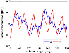
Figure 21. Radial error motion in X and Y directions determined by the multiprobe method.
Download figure:
Standard image High-resolution image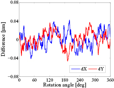
Figure 22. Differences of radial error motion between figures 19 and 21 obtained by the two methods, in X and Y directions, respectively.
Download figure:
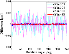
Standard image High-resolution imageIt is important to note that the repeatability of the four heads calibration results is far better than that of the three sensors measurement results in this experiment. As a comparison, figure 23 presents the differences of X and Y radial error motion between two repeat tests, for the two methods, respectively. The two differences (dX and dY) of the repeat tests for four heads setup lie within ±3 nm and are far less than those for three sensors setup. The relatively poor repeatability of the three sensors setup, which should be an important contributor to the differences in figure 22, may be mainly due to the roundness and roughness errors of the scale drum's surface where the sensors target. Since the drum roundness, also obtained by the multiprobe method, is much larger than the sub-micron level error motion, a small error on the displacement measurements will lead to a relatively large error on the error motion separation results. However, for the scanning heads measurements, owing to the high accuracy and reliability of the encoder, the angle measuring process is insensitive to the scale drum's surface quality, even when the drum is contaminated by local contamination (e.g. fingerprints, dust, water or oil drops) [4]. Therefore, to some extent, the difference in repeatability between these two setups should be reasonable in this experiment.
Figure 23. Differences of radial error motion for two tests, showing that the repeatability of the four scanning heads (4SH) setup is far better than that of the three capacitive sensors (3CS) setup.
Download figure:
Standard image High-resolution image
In summary, these experimental results obviously verify the four-scanning-heads error separation approach. The four heads method can be used not only to accurately calibrate angle encoders but also for measuring the spindle radial error motion. Further work will be focused on the verification of the error separation approach by using more than four scanning heads and with more rotary tables. On the other hand, a detailed evaluation of the uncertainty budget needs to be further studied.
6. Conclusion
A four-scanning-heads error separation technique for the self-calibration of angle encoders is presented based on Fourier approach. The goal is to separate the encoder's graduation error from the influence of axis of rotation radial error motion. To this end, the angle deviation due to the circular scale's radial motion is presented. The effect of head's angular position error on separation results is investigated, since it is one of the major uncertainty sources in this method. To avoid harmonic suppression and reduce error propagation, the optimization problem of the four scanning heads arrangement is presented. The obtained optimal arrangements should be very useful for the practical application of angle encoders. Finally, experimental tests employing four heads and three capacitive sensors are conducted. The effectiveness of the proposed method is verified by comparing the reconstructed graduation error with the results of basic self-calibration method, and comparing the separated radial error motion with the corresponding values obtained by traditional multiprobe method. The four-scanning-heads method can be used not only for calibrating angle encoders with high accuracy, but also for radial error motion measurement for some applications.
Acknowledgment
This work was supported by the Science Challenge Project (Grant No. JCKY2016212A506-0105).