

Abstract
We compute the magnetoelectric conductivity tensors in planar Hall set-ups, which are built with tilted Weyl semimetals (WSMs) and multi-Weyl semimetals (mWSMs), considering all possible relative orientations of the electromagnetic fields ( and
and  ) and the direction of the tilt. The non-Drude part of the response arises from a nonzero Berry curvature in the vicinity of the WSM/mWSM node under consideration. Only in the presence of a nonzero tilt do we find linear-in-
 terms in set-ups where the tilt-axis is not perpendicular to the plane spanned by
  and
and  . The advantage of the emergence of the linear-in-
 terms is that, unlike the various
  -dependent terms that can contribute to experimental observations, they have purely a topological origin, and they dominate the overall response-characteristics in the realistic parameter regimes. The important signatures of these terms are that they (1) change the periodicity of the response from π to 2π, when we consider their dependence on the angle θ between E and B; and (2) lead to an overall change in sign of the conductivity depending on θ, when measured with respect to the
  case.
case.
Export citation and abstract BibTeX RIS
1. Introduction
Aided by a combination of unprecedented advances in materials fabrication and theoretical analysis, the past decade has witnessed an explosive increase in the study of electronic systems having nodal points in the Brillouin zone (BZ), where two or more bands cross [1, 2]. They are called semimetals because their energy bands are neither characteristic of those in insulators (as there is no gap) nor that of conventional metals (since the density of states vanish at the nodal points). In the category of three-dimensional (3d) semimetals, the most famous examples are the Weyl semimetals (WSMs) [3, 4], whose energy dispersion relation in the vicinity of a band-crossing point is linear-in-momentum, resembling the relativistic Weyl equation (modulo the lack of strict Lorentz invariance). They are modelled by two-band Hamiltonians and host pseudospin-1/2 quasiparticles. Intriguingly, several of the defining physical properties of the Weyl fermions, such as the signature chiral anomaly (existing for odd spatial dimensions), explained by Adler–Bell–Jackiw [5, 6], continue to hold in these nonrelativistic settings involving condensed matter systems [7].
A simple generalization of the WSM is a multi-Weyl semimetal (mWSM) [8–10], whose dispersion is linear along one direction (which we choose to be the z-direction, without any loss of generality) and quadratic/cubic in the plane perpendicular to it (which we label as the xy-plane). All these 3d nodal phases exhibit nontrivial topological features in the momentum space, because each nodal point acts as a source or sink of the Berry flux, which arises from the Berry phases. Because the Berry curvature is the analogue of the magnetic field, with the Berry connection acting as a vector potential, a nodal point can be thought of as a Berry monopole carrying integer units of charge. This is the same as the Chern number, a topological invariant, obtained by integrating the Berry curvature over a closed two-dimensional (2d) surface enclosing the nodal-point. Nielson and Ninomiya's no-go theorem [11] tells us that the nodes come in pairs in a given 3d BZ, such that each pair harbours Chern numbers ±J (where J > 1), acting as source and sink of the Berry flux and adding up to zero when summed over the two nodes. Intuitively, this satisfies the requirement that the Berry curvature flux lines must begin and end somewhere within the 3d BZ, which is obtained by imposing periodic boundary conditions on the real space lattice and Fourier transforming it.
The sign of the charge gives us the chirality χ of the associated node, leading to the nomenclature of right-moving and left-moving quasiparticles, corresponding to χ = 1 and  , respectively. The values of the magnitude J of the monopole charge at a Weyl (e.g. TaAs [12–14] and HgTe-class materials [15]), double-Weyl (e.g.
  [16] and
  [17, 18]), and triple-Weyl node (e.g. transition-metal monochalcogenides [19]) are 1, 2, and 3, respectively. The chiral anomaly, mentioned in the beginning, refers to the phenomenon of charge pumping from one node to its conjugate in the presence of both electric (E) and magnetic (B) fields, which may be oriented in arbitrary directions relative to the separation of the pair of nodes. This leads to a local non-conservation of electric charge in the vicinity of an individual node, with the rate of change of the number density of chiral quasiparticles being proportional to
  [7, 20]. However, on summing over the net chiral charges for the conjugate pairs of nodes in the entire BZ, the net value comes out to be zero, thus preserving the total charge. A direct consequence of the chiral anomaly is that for
  , the longitudinal conductivity along the applied magnetic field is proportional to B2 (where
  ) and the intranode scattering time τinter, and its magnitude can be extremely large. Thus, the resistivity decreases with increasing magnetic field, leading to the observation of a large negative longitudinal magnetoresistance (LMR) in nodal-point semimetals [12, 21–25]. However, recent investigations have shown that the interplay with the orbital magnetic moment (OMM) [26, 27] and strong internode scatterings can change the sign of the LMR within the semiclassical framework [28].
The chiral anomaly leads to another effect in topological nodal phases, namely the giant planar Hall effect (PHE) [29–34], which is the appearance of a large transverse voltage when B is not aligned along E. Observation of the negative LMR and the PHE, with a specific dependence of the conductivity/resistivity tensors on the angle θ between E and B (obtained theoretically from the semiclassical Boltzmann formalism), constitutes a telltale evidence for the chiral anomaly 3 . Other smokinggun signatures of nontrivial topology in bandstructures, studied widely in the literature, include intrinsic anomalous Hall effect [35–37], planar thermal Hall effect [23, 29–32, 38–41], magneto-optical conductivity when Landau levels need to be considered [42–44], Magnus Hall effect [45–47], circular dichroism [48, 49], circular photogalvanic effect [50–53], and transmission of quasiparticles across potential barriers/wells [54–57].
Anisotropy arising from tilting of the dispersion [58, 59] is often neglected because it enters the Hamiltonian with an identity matrix, thus not affecting the eigenspinors and, hence, the topology of the low-energy theory in the vicinity of the band-crossing point. Tilting is generic in the absence of certain discrete symmetries, such as particle-hole and lattice point group symmetries (e.g. the Berry curvature of the Weyl cone does not depend on the tilt parameter). Therefore, tilted dispersion is expected to be present in WSMs/mWSMs in generic situations because of the generic nature of nodal points in 3d [60] (e.g. in a WSM with broken  [58]), made possible by their topological stability
4
. In the presence of a tilt for one of the momentum directions, which we take to be the
[58]), made possible by their topological stability
4
. In the presence of a tilt for one of the momentum directions, which we take to be the  -component in this paper, the LMR has a term with linear-in-B behaviour [61, 62]. Such linear terms may also arise when cubic-in-momentum band-bending terms (
 ) are included in the Hamiltonian [63], which break the time-reversal symmetry
  . Furthermore, in a PHE set-up, tilting leads to the presence of terms linearly dependent on B in the theoretical expressions of the longitudinal and transverse components of the magnetoelectric conductivity tensor [64–67]. This can explain the resistivity behaviour in experimental observations [68]. Our aim is to demonstrate how tilt parameters as well as the intrinsic mixed linear-nonlinear dipersion of mWSMs lead to clear signatures in PHE, which are strongly direction-dependent. We show that the
  -breaking induced by the tilt of nodes produces linear-in-B corrections, which depend on the direction of the tilt in a PHE set-up.
In this paper, we will consider an experimental set-up when a 3d semimetal is subjected to the combined effects of a static uniform external electric field E, applied along the unit vector  , and a uniform external magnetic field B, applied along the unit vector
  . If
. If  , although the conventional Hall voltage induced from the Lorentz force is zero along
  , a node with a nonzero Berry monopole charge (i.e. a nonzero Chern number) gives rise to a voltage difference along this direction. This is the PHE discussed above [23, 29, 30, 32, 38, 41, 69]. The resulting components of the conductivity tensor, which lie in the
  -plane, are commonly known as the longitudinal magnetoconductivity (LMC) and the planar Hall conductivity (PHC). Their behaviour in various experimental set-ups has been extensively investigated in the literature [34, 40, 70–78]. An untilted WSM is intrinsically isotropic and, hence, it will show the same response irrespective of how we choose to orient the
  and
and  unit vectors. However, as soon as we introduce a tilt, it introduces an anisotropy, which should give rise to a direction-dependent response. For the mWSMs, even the untilted cases are anisotropic due to the fact that they feature a hybrid of a linear dispersion along one direction and a quadratic/cubic dispersion in the plane perpendicular to it. Reference [40] discusses the changes in the zero-temperature PHE response in WSMs, induced by changing the direction of B with respect to the tilt direction, demonstrating the emergence of a linear-in-B term induced by a finite tilt. In another study [74], the authors have derived the response in such PHE set-ups using pseudospin-1 quasiparticles, described by three-band Hamiltonians, which have anisotropic hybrid dispersions analogous to the mWSMs. They did not include tilt in their computations and, hence, did not obtain any linear-in-B term like we do in our current studies.
Here we choose a tilt along the  -direction for each case, which maintains an isotropy in the xy-plane. The resulting dispersion is shown schematically in figure 1. With these considerations in mind, we have three distinct configurations for applying E and B in a planar Hall set-up, which are illustrated in figure 2. In the first two set-ups, which we label as I and II,
  is set perpendicular to the
  -axis, which we have chosen to be the x-axis. In set-up I, we orient
  to lie in the xy-plane, while in set-up II, we orient
  to lie in the zx-plane. In the last set-up, which we denote as set-up III,
  is set parallel to the tilt-axis and
  lies in the zx-plane. In each case,
  makes an angle θ with
  , which is not
  in general for observing the PHE. We will employ the semiclassical Boltzmann transport formalism, which works well for small magnetic fields and small cyclotron frequency
  [where
  is the effective mass with the magnitude
  [79], with me
denoting the electron mass] such that the Landau quantization can be ignored. The regime of validity is given by
[79], with me
denoting the electron mass] such that the Landau quantization can be ignored. The regime of validity is given by  , where µ is the chemical potential/Fermi level.

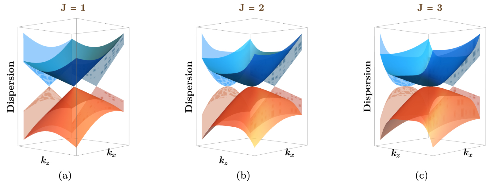
Figure 1. Schematic dispersion of a single tilted node [cf. equation (1)] in a (a) Weyl, (b) double-Weyl, and (c) triple-Weyl semimetal, plotted against the  -plane. The tilting is taken along the
 -direction, along which the dispersion depends linearly on the momentum. The double(triple)-Weyl node shows an anisotropic hybrid dispersion with a quadratic(cubic)-in-momentum dependence along the
 -direction. The direction-dependent features are depicted more clearly with the help of the projections of the dispersion along the respective momentum axes.
Download figure:
Standard image High-resolution image
Figure 2. Schematics of the three set-ups that we have used for investigating the planar Hall effect in WSMs/mWSMs, showing the relative orientations of the external homogeneous electric E (red arrow) and magnetic B (blue arrow) fields, which we label as (a) set-up I, (b) set-up II, and (c) set-up III, respectively. The plane containing the E and B vectors (making an angle θ with each other) in each set-up has been highlighted by a background colourshading. Each type of semimetal has a direction along which the dispersion is linear-in-momentum, which we have chosen to be the z-direction, which is also the axis with respect to which the dispersion has a tilt [cf. figure 1 and equation (1)].
Download figure:
Standard image High-resolution imageIn the presence of  , the Onsager-Casimir reciprocity relations [80–82] constrain the B-dependence of the conductivity tensor
  (where
  are the indices denoting the tensor components along the axes of a chosen set of Cartesian coordinates) to be
  and
and  , with
  denoting an axis along
  and
and  aligned perpendicular to
  . However, a finite tilt breaks
  , thus opening up the possibility of terms which are linearly dependent on B. An in-depth analysis of the effects of spatial symmetries on PHE can be found in reference [83].
The paper is organized as follows: In section 2, we introduce the low-energy effective Hamiltonian in the vicinity of a tilted WSM/mWSM node. In section 3, we outline the steps to compute the conductivity tensor. Section 4 is devoted to demonstrating the explicit expressions for the longitudinal and transverse components of the conductivity tensor, and illustrating their behaviour in some relevant parameter regimes. Finally, we conclude with a summary and outlook in section 5. In all expressions that follow, we will use the natural units by setting the reduced Planck's constant ( ), the speed of light (c), and the Boltzmann constant (kB
) to unity. We also show the representative values of the various parameters, appearing in the Hamiltonians and the expressions for the conductivity tensors, using both the SI and the natural units, in table 1.
), the speed of light (c), and the Boltzmann constant (kB
) to unity. We also show the representative values of the various parameters, appearing in the Hamiltonians and the expressions for the conductivity tensors, using both the SI and the natural units, in table 1.
Table 1. We list the parameter regimes which we have used in plotting the components of conductivity tensor. Using the relation  , we get
  ,
,  , and
, and  . In terms of natural units, we need to set
  , and
, and  . In our plots, we have used
  (from the table entry), leading to
  eV−1 and
  eV−2. For J = 2 and J = 3,
  has been set equal to v0 for the sake of simplicity, while for the isotropic dispersion (modulo the tilt) of J = 1, we are constrained to have
  .
.
| Parameter | SI Units | Natural Units |
|---|---|---|
| v0 from references [79, 86] |
 m s−1 m s−1
| 0.005 |
| τ from references [79, 86] |

| 151.72 eV−1 |
| T from references [32, 68] |

|

|
| B from [87] |

|

|
| µ from references [62, 74] |
 eV eV |
 eV eV |
2. Model for a tilted WSM/mWSM node
In the vicinity of a nodal point with chirality χ and Berry monopole charge of magnitude J, the effective continuum Hamiltonian is given by [8, 9, 19]

where  , v0(
, v0( ) is the Fermi velocity along the z-direction(xy-plane), k0 is a material-dependent parameter with the dimension of momentum, and η is the tilt parameter (which is taken along the
  -direction). Henceforth, we will consider the positive-chirality node by setting χ = 1. The eigenvalues of the Hamiltonian are given by

where the value 1(2) for s represents the upper(lower) band. The Hamiltonian for a WSM node is isotropic in absence of the tilt, which is recovered from  by setting J = 1 and
  . Figure 1 shows the schematic dispersion against the
  -plane. In this paper, we restrict ourselves to the type-I phases such that
  , which gives a Fermi point, an electron-pocket, or a hole-pocket, depending on whether the chemical potential cuts the nodal point, the upper band, or the lower band.
The Berry curvature (BC) associated with the sth band is given by [38, 84]

where the set of indices  takes values from
  , and is used to denote the components of the Cartesian vectors and tensors. The BC arises from the Berry phases generated by
  , where
  denotes the set of orthonormal Bloch cell eigenstates for the single-particle Hamiltonian
  . On evaluating the expressions in equation (3) using equation (1), we get

The Bloch velocity vector for the quasiparticles occupying the sth is given by

We find that the BC is independent of the tilt, as expected, while the z-component of  gets shifted due to the tilt term. In this paper, we will take a positive value of the chemical potential µ such that it cuts the conduction band with s = 1. Henceforth, we use the notations
  ,
,  , and
, and  , in order to avoid cluttering.
3. Magnetoelectric conductivity
We use the semiclassical Boltzmann formalism to find the form of the magnetoelectric conductivity tensor  in a generic PHE set-up. We employ a relaxation-time-approximation for the collision integral and, furthermore, assume a momentum-independent relaxation time τ, which we treat as a phenomenological constant. We focus on the scenario when the internode scattering amplitude is negligible compared to the intranode scattering amplitude, which suppresses any relaxation towards equal occupation of the two nodes in a conjugate pair, thereby enhancing signatures of the chiral anomaly [23, 24]. Therefore, τ corresponds solely to the intranode scattering time. The derivation is outlined in detail in references [34, 85]. The final expression for conductivity, contributed by the conduction band at the node with positive chirality, is given by

where

is the phase-space-factor which takes into account the modified density of states in the presence of an external magnetic field, and

represents the equilibrium distribution function of the fermionic quasiparticles (with  ). We have taken the charge of each quasiparticle to be −e, where e is the magnitude of the charge of an electron. The first part, labelled as
  , represents the 'intrinsic anomalous' Hall effect [35–37]. The second part
  is the Lorentz-force-contribution to the conductivity. The last term
  is the Berry-curvature-related conductivity coefficient. For a momentum-independent τ,
  is an order of magnitude smaller than the other terms [30] in a typical WSMs/mWSM and, hence, we neglect it. Furthermore, we are not interested in
  because, together with the contribution from the node with opposite chirality, it leads to an overall zero contribution when we sum the conductivity coming from the two nodes.
For the ease of calculations, we decompose σpq into four parts as follows:

We find that  ,
,  , and
, and  go to zero if the BC vanishes. We will expand
  in powers of
  , restricting to the regime with a weak strength of the magnetic field, and keep terms upto order
  in the expressions for
  .
.
Now we outline the details for obtaining the final form of the LMC for the set-up I, discussed in section 4.1. For this case, we have to set  and
and  . Hence, the LMC is given by

where

Keeping terms upto  , we obtain

Changing the integration variables as

leads to  , where
  in general (i.e., irrespective of whether we consider the upper or the lower band). Since we are considering s = 1 here, we have

where

Following a similar sequence of steps, the first part of the PHC is given by

In order to evaluate  , we employ the Sommerfeld expansion

which is valid in the regime  . Plugging in the above expression, we get

The last step is to perform the γ-integral, using the identity

where  is the regularized hypergeometric function [88]. Implementing this, we finally get


where  is independent of the magnetic field and is usually referred to as the Drude contribution. The Drude part arises from the j = 0 term in the summation appearing in the integrand on the right-hand-side of equation (17). The j = 1 term vanishes identically because of the presence of odd powers of
  or
or  . The j = 2 term gives rise to the second nonzero part
  , whose origin is from a nonzero BC. For the case of PHC, we find that j = 0 and j = 1 terms vanish while performing the φ-integration, and j = 2 provides the only nonzero contribution to
  , which has a purely topological origin. Although we do not have any linear-in-B term for this case, we will find it in the other set-ups. Proceeding in the way explained above, we obtain the final expressions for
  ,
,  ,
,  ,
,  ,
,  , and
, and  , the steps of which are not very necessary to write down explicitly.
To show the emergence of the linear-in-B, we include here the starting expression for the first part of the LMC of set-up II, discussed in section 4.2. This is captured by

where

For j = 0, we get the Drude part, which is the same as equation (20) obtained for set-up I. For j = 1, we now have a nonvanishing contribution coming from the φ-independent part of  , because, unlike the LMC in set-up I, the integrand here has even powers of
  . This leads to a term linear-in-B. For j = 2, we obtain the usual B2-dependent terms, which exist even in the absence of a nonzero tilt.
The intermediate steps for the remaining tensors are omitted here, as they are similar to the derivations demonstrated above. In any case, we provide the full final expressions for each set-up in the corresponding subsections of section 4.
4. Results
In this section, we explicitly write down the expressions for the nonzero components of the magnetoelectric conductivity tensor for the three distinct set-ups shown in figure 2. We also illustrate their behaviour by some representative plots, and discuss the physical implications of their characteristics. Before delving into the explicit expressions, we have summarized the results in table 2 for the ease of a quick comparison.
Table 2. Summary of the key characteristics of the response for the three distinct set-ups, showing the B-dependence of the terms appearing in the final expressions.
| Set-up I | Set-up II | Set-up III | |
|---|---|---|---|
| LMC | terms proportional to B0 and B2 | terms proportional to B0, B, and B2 | terms proportional to B0, B, and B2 |
| PHC | terms proportional to B2 | terms proportional to B and B2 | terms proportional to B and B2 |
4.1. Set-up I
In set-up I, as shown in figure 2(a), the tilt-axis is perpendicular to the plane spanned by E and B. Since there exists a rotational symmetry of the dispersion of each semimetallic node within the xy-plane, the exact directions of E and B will not matter. What matters is the angle between  and
and  . Hence, without any loss of generality, we choose
  and
and  .
.
4.1.1. LMC.
The full expression for the LMC is given by

where  has already been shown in equation (19), and

From equation (20), we find that the Drude part is an even function of η. The remaining parts, dependent on a nonzero BC, are functions of η2, thus making them even functions of η as well. For this set-up, only even powers of B appear, and we do not obtain any part linearly varying with B, similar to the untilted cases [32, 44]. Also important to note is that the BC-dependent part is independent of the chirality of the node. This is because the terms in the integrand contributing to a nonzero result involve only even powers of the components of the BC (which is proportional to χ). As a consequence of all these observations, we conclude that, if we sum over the contributions from a pair of conjugate nodes, they add up, irrespective of whether of the two nodes are tilted in the same or opposite directions. Figure 3 illustrates the behaviour of the LMC for some representative parameter regimes.

Figure 3. Set-up I: Variation of the LMC (in units of eV2) with (a) the angle θ and (b) the magnitude B (in units of eV2) of the magnetic field. For all the plots, we have set  , τ = 151 eV−1, µ = 0.1 eV, and β = 1160 eV−1.
Download figure:
Standard image High-resolution image4.1.2. PHC.
The PHC does not have a Drude part and is entirely caused by a nonzero BC. Explicitly, it takes the form:

σyx
is a function of η2 and B2, and it arises entirely from even powers of the components of the BC (making it independent of the chirality of the node). Hence, analogous to the PHC, it will give the same contribution from each conjugate node, irrespective of the sign of the tilt. However, unlike the LMC, the PHC vanishes when θ equals zero or  . Figure 4 demonstrates the characteristics of σyx
for some representative parameter regimes.
. Figure 4 demonstrates the characteristics of σyx
for some representative parameter regimes.

Figure 4. Set-up I: Variation of the PHC (in units of eV2) with (a) the angle θ and (b) the magnitude B (in units of eV2) of the magnetic field. For all the plots, we have set  , τ = 151 eV−1, µ = 0.1 eV, and β = 1160 eV−1.
Download figure:
Standard image High-resolution imageThe PHC components do not show discernible changes with β, while the LMC does to some extent. Hence, in figure 9, we illustrate the variations of LMC with β.
4.2. Set-up II
In set-up II, as shown in figure 2(b), the tilt-axis is perpendicular to E, but not to B. We choose  and
and  .
.
4.2.1. LMC.
The full expression for the LMC is given by

where σDrude is the same as shown in equation (20),


and

The parts other than the Drude contribution originate from a nonzero BC. In this case, we find that  has a part which varies linearly in η as well as B, that originates from the contribution of a term in the integrand which is proportional to the BC (and, consequently, the chirality χ of the node). This part, being proportional to
  , will cancel out when summed over the two nodes in a conjugate pair, if the tilt-signs are the same. The remaining terms are quadratic in both η and B, and are independent of the chirality. Hence, these parts add up irrespective of the sign of the tilt. Figure 5 illustrates the behaviour of the LMC for some representative parameter regimes. In particular, the periodicity of the curves, as functions of θ, changes from π to 2π as soon as a nonzero tilt is introduced. Furthermore, figure 5(b) shows that the linear-in-B parts dominate for a nonzero tilt, with the magnitude increasing with increasing J [because of the factor
  , which monotonically increases with J]. Most importantly, the dominant B-linear terms lead to a change in the overall sign of the LMC for various ranges of θ, when measured with respect to the B = 0 case. We also capture the η-dependence in figure 8.

Figure 5. Set-up II: Variation of the LMC (in units of eV2) with (a) the angle θ and (b) the magnitude B (in units of eV2) of the magnetic field. For all the plots, we have set  , τ = 151 eV−1, µ = 0.1 eV, and β = 1160 eV−1.
Download figure:
Standard image High-resolution imageLet us elaborate a bit more on the appearance of the term proportional to  . When the system is subjected to homogeneous external fields, then, in the absence of any other scale in the problem, the Onsager-Casimir reciprocity relation
  [80–82] forbids any term in the LMC to be linear in B, unless the change of sign of B is compensated by a change of sign in another parameter in the system. The tilt vector, defined by
  in this paper, provides us with such a compensating sign, such that we have now the identity
  , thus fulfilling the Onsager-Casimir constraints [63]. This allows the linear-in-B to appear in
  , with the corresponding part of the magnetocurrent being proportional to
  , in agreement with the findings of reference [40] for WSMs at T = 0. Because
  is perpendicular to t in this set-up, the linear contribution vanishes for θ = 0. We note that this term has a nontrivial dependence on the chemical potential and the temperature, via the term
  , for J ≠ 1 (because, of course, ϒ0 = 1). The fact that the µ-dependence disappears for J = 1 is consistent with the WSM studies of reference [40].
4.2.2. PHC.
Analogous to set-up I, the PHC does not have a Drude part and is entirely caused by a nonzero BC. Explicitly, it takes the form:

where


and

Here too we find the emergence of terms proportional to  [cf. the first terms in
  and
and  ], but without having any dependence on µ or β for any J (unlike the LMC). Moreover, they are directly proportional to J as well. The corresponding part of the magnetocurrent is proportional to
  , in agreement with the findings of reference [40] for WSMs at T = 0. Therefore, this linear contribution vanishes when
  . Figure 6 demonstrates the characteristics of the full PHC for some representative parameter regimes, where we find the linear term to be dominating the overall behaviour of the curves for tilted nodes, with the magnitude increasing with increasing values of J. A nonzero tilt also changes the periodicity of the curves, as functions of θ, from π to 2π, and causes an overall change in the sign of the PHC for various ranges of θ, when measured with respect to the B = 0 case. We depict the η-dependence in figure 8.

Figure 6. Set-up II: Variation of the PHC (in units of eV2) with (a) the angle θ and (b) the magnitude B (in units of eV2) of the magnetic field. For all the plots, we have set  , τ = 151 eV−1, µ = 0.1 eV, and β = 1160 eV−1.
Download figure:
Standard image High-resolution imageThe PHC components do not show discernible changes with β, while the LMC does to some extent. Hence, in figure 9, we illustrate the variations of LMC with β.
4.3. Set-up III
In set-up III, as shown in figure 2(c), the tilt-axis is parallel to E, such that  , and
, and  .
.
4.3.1. LMC.
The full expression for the LMC is given by

where


We find that there is a B-independent Drude part, viz.,  , whose form is different from equation (20). However, similar to
  ,
,  is an even function of η (independent of χ) and, hence, independent of the sign of the tilt. Analogous to the LMC in set-up II, we find that
  contains a linear-in-B term, whose behaviour goes as
  . In addition, there is another linear-in-B term coming from
  and
and  with the dependence
  . None of these B-linear terms has any µ- or T-dependence and, while summing over the conjugate nodes of opposite chiralities, the net result will be nonzero only for tilting in opposite directions. The part of the electric current arising from them is proportional to
  , and the identity
  makes it possible to satisfy the Onsager-Casimir reciprocity relations. The remaining terms of σzz
are quadratic in B, contain even powers of η, and are independent of the chirality of the node. All the non-Drude terms vanish when
makes it possible to satisfy the Onsager-Casimir reciprocity relations. The remaining terms of σzz
are quadratic in B, contain even powers of η, and are independent of the chirality of the node. All the non-Drude terms vanish when  and have an overall 2π(π)-periodicity in θ for nonzero(zero) η. All these are accompanied by an overall change in sign of the LMC for various ranges of θ, when measured with respect to the B = 0 case. The typical characteristics of the LMC are captured in figure 7 via some representative parameter regimes. We also capture the η-dependence in figure 8. Figure 9 illustrates the variations of the LMC with β.

Figure 7. Set-up III: Variation of the LMC (in units of eV2) with (a) the angle θ and (b) the magnitude B (in units of eV2) of the magnetic field. For all the plots, we have set  , τ = 151 eV−1, µ = 0.1 eV, and β = 1160 eV−1.
Download figure:
Standard image High-resolution image
Figure 8. Comparison of the η-dependence of the σpq
components (in units of eV2) for the two set-ups (indicated in the plotlabels) in which we find linear-in-B terms. For all the plots, we have set B = 3 eV2,  ,
,  , τ = 151 eV−1, µ = 0.1 eV, and β = 1160 eV−1. The curves in the upper(lower) panel have the η = 0(B = 0) parts subtracted off from the full response.
Download figure:
Standard image High-resolution image
Figure 9. Comparison of the variations of the LMC components (in units of eV2) as functions of β (in units of eV−1) over various set-ups (indicated in the plotlabels). For all the plots, we have set B = 3 eV2,  ,
,  , τ = 151 eV−1, µ = 0.1 eV, and η = 0.5. The curves have the T = 0 parts subtracted off from the full response.
Download figure:
Standard image High-resolution image
4.3.2. PHC.
As for the PHC, we have the simple relation

Hence, we get a linear term similar to set-up II. The only difference is that here the magnetocurrent, arising from the B-linear term, is proportional to  .
.
4.4. Other set-ups and generic conclusions
Let us consider another distinct set-up where we have  and
and  . This is not a planar Hall set-up, as E and B are perpendicular to each other, and, hence, only gives rise to the transverse (or Hall) conductivity. This also implies that the Drude part has to be zero. The PHC components are explicitly given by

where

The B2-dependent terms are identically zero in this case and, to any order in B, the final expression is proportional to the tilt η. This results from the fact that only odd powers of B exist upto any order.
The components of σpq
in all other possible configurations of PHE set-ups can be obtained from the ones shown here. For example, if we take  and
and  , which is the generalization of set-up II with B now having a nonzero y-component as well, the extra PHC component σyx
is the same as that obtained for set-up I, after making the replacement
, which is the generalization of set-up II with B now having a nonzero y-component as well, the extra PHC component σyx
is the same as that obtained for set-up I, after making the replacement  . Another example is when we choose
  and
and  — the corresponding PHC expressions are:

Hence, our results exhaust all the distinct cases that can arise, taking into account all possible relative orientations and direction-dependence.
5. Summary and outlook
The PHE has been measured in numerous experiments — a few examples involve materials like ZrTe5 [68, 89], TaAs [90], NbP [69], NbAs [69], and Co3Sn2S2 [91], hosting Dirac and Weyl nodes. In particular, signatures of linear-in-B behaviour have been reported in their data. Reference [12] has presented experimental evidence confirming the giant LMR resulting from the chiral anomaly in the time-reversal-invariant Weyl semimetal material  , and has shown that the response undergoes a sign change as the direction of the magnetic field is rotated. In reference [68], by considering
  , the authors have shown the variation of the planar Hall resistivity with the angular orientation of the applied magnetic field. The experimental results in reference [92] show the angular variations of both the longitudinal and the planar Hall resistivity components in the Heusler Weyl semimetal
  . The measurements reported in [93] show the presence of both linear-in-B and B2-dependent terms in the response for Cd3As2. In order to find the origins of the experimental data, as well as to motivate further investigations, we have delved into the characterization of the magnetoelectric conductivity tensors in the context of planar Hall set-ups built with tilted WSMs and mWSMs, considering various relative orientations of the electromagnetic fields and the direction of the tilt.
One instance of the importance of our studies can be motivated as follows. We know that the response in PHE is not solely generated by the chiral anomaly and nonzero BC in the nodal-point semimetals. In fact, it can also have nontopological origins from magnetic order, spin-orbital coupling, and trivial in-plane orbital magnetoresistance [94]. The PHE in nonmagnetic WSMs/mWSMs is dominated by the BC and chiral anomaly contributions only for materials with a relatively small orbital magnetoresistance [92]. However, in magnetic WSMs/mWSMs, the response is dominated by the part originating from the Berry phase, because the anisotropic magnetic resistance (caused by different in-plane and out-of-plane spin scatterings) induced in ferromagnetism is very small in comparison. The topological and nontopological origins of the PHE, discussed above, cannot always be clearly distinguished in experiments, because the experimentally observed quadratic-in-B magnetoconductance arises via both mechanisms. To remedy the situation, we can use the fact that the BC gives rise to a linear-in-B term in magnetoconductance if the node is tilted. In fact, our results show that this term dominates in suitable parameter regimes, and increases in magnitude as the magnitude of the monopole charge J increases. Most importantly, the dominant B-linear terms lead to a change in sign of the magnetoconductance depending on the value of θ, when measured with respect to the B = 0 case.
If we consider a 3d Dirac semimetal with the Hamiltonian [95]

where
σ
and
τ
denote the vectors of the three Pauli matrices acting on two different symmetry-operator-spaces, we find that the Dirac node comprises a pair of doubly-degenerate cones with dispersions ±k. Adding a perturbation of the form  splits the Dirac node into two distinct Weyl nodes, separated in the kx
-momentum direction. A single Weyl node has the disperion relation
splits the Dirac node into two distinct Weyl nodes, separated in the kx
-momentum direction. A single Weyl node has the disperion relation  , where
 ![$E_{\text{weyl},s} = \sqrt{\left [ k_x + (-1)^s\, \delta \right ]^2+k_y^2+k_z^2}$](https://content.cld.iop.org/journals/0953-8984/36/27/275501/revision2/cmad38faieqn184.gif) , and
, and  labels the two Weyl nodes. On linearizing the momentum dependence around each node, the problem reduces to a
  Hamiltonian
  in the vicinity of each node, where χ denotes the chirality of the node in consideration. In the experimental results reported in papers like reference [96], Dirac semimetals such as Na3Bi are considered. There, an applied magnetic field breaks the time-reversal symmetry and separates the two nodes due to the spin Zeeman energy. Now, if an electric is applied parallel to the magnetic field, an axial current is generated, which is observed as a large negative LMR. Hence, our results are applicable to experimental observations on Dirac semimetals, when the node gets split into two Weyl nodes due to an external perturbation (e.g., the applied magnetic field).
We would like to point out that we have not considered the OMM in order to make it possible to obtain closed-form expressions from the integrals, and to identify the features (e.g., emergence of the linear-in-B dependence) originating solely from the effects of tilt. This is justified by the fact that the OMM, in the limit of negligible internode scatterings, is not expected to change the qualitative results, and has been neglected in the earlier studies as well [30, 40, 62, 64, 75]. However, in future we will determine how a combination of OMM and significant internode scatterings modify the response, as indicated in references [28, 31]. In order to capture the correct physics, we must go beyond the relaxation-time approximation [28].
In the future, it will be worthwhile to study the influence of a strong quantizing magnetic field, when Landau level formation cannot be ignored [43, 44, 76, 97]. The behaviour of the magnetoconductivity in the presence of strong disorder as well as many-body interactions [53, 98–103] will take us into the regime where interactions cannot be ignored. Another possible direction is to investigate the response resulting from an additional time-periodic drive [41, 55, 56] applied on the system (e.g., by shining a beam of circularly polarized light).
Acknowledgments
RG is grateful to Ram Ramaswamy for providing the funding during the initial stages of the project. IM's research leading to these results has received funding from the European Union's Horizon 2020 research and innovation programme under the Marie Skłodowska-Curie Grant Agreement Number 754340.
Data availability statement
No data was used for the research described in the article.
Footnotes
- 3
PHE is also observed in ferromagnets, but its value is very small.
- 4
The WSM/mWSM nodes are very robust, requiring only the discrete translational invariance of the crystal.