
Abstract
We use video microscopy to study the full capture process for colloidal particles transported through microfluidic channels by a pressure-driven flow. In particular, we obtain trajectories for particles as they move from the bulk into confinement, using these to map in detail the spatial velocity and concentration fields for a range of different flow velocities. Importantly, by changing the height profiles of our microfluidic devices, we consider systems for which flow profiles in the channel are the same, but flow fields in the reservoir differ with respect to the quasi-2D monolayer of particles. We find that velocity fields and profiles show qualitative agreement with numerical computations of pressure-driven fluid flow through the systems in the absence of particles, implying that in the regimes studied here particle-particle interactions do not strongly perturb the flow. Analysis of the particle flux through the channel indicates that changing the reservoir geometry leads to a change between long-range attraction of the particles to the pore and diffusion-to-capture-like behaviour, with concentration fields that show qualitative changes based on device geometry. Our results not only provide insight into design considerations for microfluidic devices, but also a foundation for experimental elucidation of the concept of a capture radius. This long standing problem plays a key role in transport models for biological channels and nanopore sensors.
Export citation and abstract BibTeX RIS
1. Introduction
The efficient transport of particles through channels and pores is essential to the function of a diverse range of natural and synthetic systems, from blood vessels and the nuclear pore complex to filters, catalysts and nanopore sensors. As such, significant efforts have been made to understand the dynamics of particles in these confining geometries [1–8], particularly for the case of single-file diffusion [9–12]. Yet, analyte flux through a system is often limited not by the rate of movement through the channel, but by the rate at which a transported species enters into, or is captured by, a channel or pore [13]. This rate typically depends on a complex interplay of phenomena, including the concentration of the transported species, details of the geometry, interparticle and particle-pore interactions, and the strength and nature of external driving forces. Additionally, the entropic barrier associated with movement into a confining geometry plays a key role, especially for the transport of macromolecules [14]. Manipulating one or more of these parameters to enhance transport rate has been exploited by both biological channels [15] and synthetic systems [16, 17].
For driven transport through channels, the capture and transport process can be described by three steps: diffusion of a molecule from the bulk to a position that lies close enough to the pore to feel the external potential, funnelling of the molecule towards the pore by the external field and, finally, transition of the molecule into the channel opening [14, 16, 18, 19]. The relative importance of each of these steps depends sensitively on details of the system. For example, for polymer transport the final step is crucial as it involves the polymer adopting a conformation that allows it to thread through the channel. It has thus been widely considered in the context of sensing and sequencing applications [16]. In contrast, the first two stages of the process are less well understood, as they are difficult to directly observe in molecular level experiments associated with short length and time scales. Yet, for systems where diffusion to capture is the limiting process, it is precisely these first two stages that are most relevant. To describe the early stages of the capture process, most studies invoke the concept of a capture radius; the distance from the pore at which the dynamics of the molecule transition from being dominated by diffusion to being dominated by drift. Recent theoretical and simulation work has shown, however, that the capture radius is difficult to define and interpret, even in relatively simple scenarios [13]. Experimentally, in recent years colloidal models have provided significant insight into confined transport processes [4–7, 9–12, 20, 21]. In cases where both reservoir and channel have been studied, however, diffusion of particles out-of-plane in the reservoirs has made tracking of full particle trajectories from bulk to channel very challenging, inhibiting this study of the full capture process.
Theoretically, to elucidate the nature of diffusive and advective transport processes an important concept is the Péclet number [22]; a non-dimensional ratio between advective and diffusive transport rates, here defined as:

for some drift velocity u, particle radius r and diffusion coefficient D. Yet, unambiguous definition of a Pèclet number in confined systems with heterogeneous dynamics i.e. where length scales and time scales spatially vary is not trivial [13], since with multiple relevant length scales there are many dimensionless ratios which could be included in a definition of Pe. Within well defined parts of such systems (e.g. inside the channel away from the entrances) there are few enough length scales to make the problem tractable. For instance, if the particle resides within a channel of length L, a comparison of the time scales for diffusive and advective transport ( ,
,  ) indicates that we see advection dominate when
  . Notably, this advective transport condition corresponds to
  , considerably less than one. Clearly, in such a limited case, the solution is to use L as the characteristic length scale in the definition of Pe. However, such a definition then loses meaning outside of the channel environment. It is precisely at the thresholds between such parts of the system where non-trivial behaviour is observed. In our case, this is the region at the pore mouth where capture occurs. As such, for a system in which you can fully observe and measure all particles at all times, the most complete understanding of the system will come from considering the individual particle motion in detail.
Here, we use video microscopy to study the full capture process for colloidal particles gravitationally confined to a monolayer and driven through microfluidic channels by a pressure-driven flow (figure 1). In particular, we study in detail properties of particle trajectories as they move from the bulk into confinement in microfluidic devices with two different height profiles ('2D' vs '3D' in figure 2). The different height profiles allow us to investigate the capture properties for different fluid flow speeds in the reservoir whilst keeping the same flow speed in the channel. We compared the measured particle speeds to fluid flow profiles, computed for systems without any particles present, allowing us to probe the effect of particle interactions. Good qualitative agreement between the computed fluid flow and experimental particle speeds allow us to conclude that interparticle interactions do not significantly influence the particle transport at the particle concentrations considered here (∼10%). We then consider particle flux through the channel, observing for the '2D' geometry an apparent long-range attraction to the pore, in contrast to more diffusion-to-capture-like behaviour for the '3D' geometry. This highlights how subtle changes to geometry can qualitatively change capture behaviour. Finally, to explore these qualitative differences in behaviour we map the concentration fields for both geometries at a variety of flow speeds. For both geometries we observe a reduction of the particle concentration in the channel. Here we find for our '2D' geometry a reduction in concentration in the channel with respect to the bulk ∼50% independent of flow speed. In contrast, for the '3D' geometry the concentration decrease is much greater and depends on flow speed with an empirical relationship of  . Our results not only provide insight into design considerations for microfluidic devices, but also into the concept of a capture radius. This long standing problem plays a key role in transport models for biological channels and nanopore sensors.
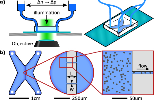
Figure 1. Observing particle capture into microfluidic channels by imposing pressure driven flows. (a) Schematic diagram of the set-up, illustrating the application of a pressure driven flow by positioning macroscopic reservoirs above the PDMS chip. (b) Geometry of reservoirs and microfluidic channels at different magnifications.
Download figure:
Standard image High-resolution image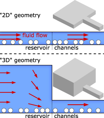
Figure 2. The two different chip geometries considered here. Top: the '2D' geometry, where the channels are the same height as the reservoirs. Bottom: the '3D' geometry, where the reservoirs are ∼4× deeper than the channels. All heights in the figure are to scale.
Download figure:
Standard image High-resolution image2. Methods
2.1. Colloidal model system
Microfluidic chips are designed to include two reservoirs linked by an array of channels with length  m, and width and height
  m. Each microscopic reservoir is connected to a macroscopic reservoir outside the chip via tubing (figure 1). The relative heights of the macroscopic reservoirs can be varied to induce a pressure difference across the channels, causing a fluid flow through the chip. Since the total pressure difference between the two macroscopic reservoirs drives flow through all the channels and sundry parts of the system, the controlled value is the pressure drop over the single channel being measured, for which particle speed within the channel is used as a proxy; since the channels are always the same shape there is a one-to-one correspondence between the two quantities. Two different chip designs are used with respect to the height of the reservoirs: in the first, reservoirs have a height equal to that of the channels ('2D'), whilst in the second the reservoirs have a height of approximately four times that of the channels, at 30 µm ('3D'). The difference between the two geometries is illustrated in figure 2. Microfluidic chips are fabricated by replica moulding in poly-dimethylsiloxane (PDMS), before plasma bonding of the PDMS component to a glass slide coated with a thin layer of PDMS. Moulds are fabricated using standard photo-lithography techniques on silicon wafers [23]. Data is recorded at a rate of 20 fps using a custom-built inverted optical microscope, imaging an area of 200 µm at a resolution of
  pixels, making each pixel a square of side 0.157 µm. An unprocessed section of a typical image of the system is shown in figure 3 (inset).

Figure 3. Measured trajectories of particles in the system. 62 distinct trajectories are shown, with the particles moving from the reservoir into the channel; the chip shown here is of the '3D' geometry, with a packing fraction of ∼7% and the mean particle speed in the channel being ∼39 µm s−1. Inset: the area around the channel entrance from a single frame of data, showing the colloids (scale same as main panel).
Download figure:
Standard image High-resolution imageThe colloidal suspension consists of carboxylate-functionalised melamine formaldehyde particles with a diameter of 2.79 µm dispersed in deionised water. Previous studies have shown the particles are an excellent experimental realisation of hard spheres [24–26]. When loaded into the microfluidic device, the high density of the particles with respect to the solvent results in their rapid sedimentation onto the base of the chip where they are gravitationally confined to a monolayer (gravitational height of particles ∼0.08 µm). As such, all particles, both within the channels and the reservoirs, can be imaged at all times, irrespective of whether the reservoir height is comparable to the particle diameter or much larger. Crucially, this allows the capture process, i.e. the transition of a particle from a bulk to confined environment, to be visualised in its entirety for each particle, in contrast to previous studies in which particles in the reservoirs can diffuse out-of-plane [21]. The packing fraction of the quasi-two dimensional monolayer of colloids in both the upstream and downstream reservoirs is  –0.12 and does not vary significantly over the time span of the experiments. We note that, for this range of packing fractions and the driving forces used, we do not observe clogging of the channels as seen in other work [27, 28].
2.2. Image analysis
Particle trajectories are obtained from images using standard particle tracking routines implemented in python, in particular, the trackpy package based upon the Crocker–Grier algorithms for feature finding and linking [29, 30]. In brief, each video contains 100 000–130 000 frames of  pixels, covering an area of
  m. For each frame we first subtract a background image obtained as the average over approximately 20% of the total frames taken uniformly from the whole video. This removes features associated with the channel walls from the images allowing for easier identification of the particle positions. We use adaptive linking to build trajectories from these positions, which handles the problem posed by highly spatially heterogeneous flow fields—and thus particle displacements—in our system. Adaptive linking begins with a large search distance for features in the previous frame which may correspond to features in the current frame, then iteratively reduces that range on a per-particle basis until the computation is feasible, since the linking time is
  for a subnet containing n particles [29, 30]. These steps were performed in parallel on 1000 frame sections of the whole video, and the results from each section were then 'stitched' together, which greatly sped up the whole process and avoided problems with computer memory. Typical trajectories for particles entering a channel in a 3D chip for are shown in figure 3.
Velocities  at each position
  in a particle's trajectory are estimated by
  , i.e. the displacement between the previous and following positions. Whilst this results in an average over two time steps, it allows the clear association of a single velocity with a single position. When a bulk packing fraction is quoted (or used for normalisation), it was calculated by averaging over a rectangle with the full height of the image (160 µm) and width 70 µm, located at the far left of the image (see figure 3).
2.3. Péclet number
As noted earlier, we define the Péclet number, Pe, as:  , for some drift velocity u, particle radius r and Diffusion coefficient D. For the particles considered in this work, with
  m. The diffusion coefficient was measured to be
  , less than that predicted by the Stokes–Einstein relation due to the hydrodynamic interactions with the system floor. These values together give
  s−1.
s−1.
2.4. Flow computations
Fluid flow profiles without the presence of particles were computed using COMSOL for comparison with the particle velocity fields measured by our experiments. Due to the low Reynolds number,  of the system, we could use creeping flow dynamics, solving the Stokes equations for flow through a single channel of length 100 µm, width 8 µm and height 8 µm connecting two reservoirs of
  m and height either 8 µm (2D) or 30 µm (3D). No-slip boundary conditions were used for the walls corresponding to physical walls, and open boundaries with constant pressure P used for the remaining walls, with
  on the upstream side, and P = 0 on the downstream side. The flow speeds shown have been evaluated in the plane
  m, which corresponds to the plane of the centres of the sedimented particles. In the experimental system the particles will strongly perturb the fluid flow, so having a measure of the unperturbed flow from these computations allows us to assess the effect of the particle interactions.
3. Results and discussion
First, we consider the spatial variation of the particle velocity in the vicinity of the channel entrance. Figure 4(a) shows heatmaps of the particle speed for a single experiment in both the 2D and 3D geometries, as illustrated in figure 2. The velocity field is calculated by averaging the instantaneous velocity of all particle trajectories passing through a square bin with length 1.26 µm (8 pixels) at each spatial position. Due to the low Peclet number in the reservoir, streamlines are not well defined and so are not shown. The particle speed within the channel is similar in each case, peaking at 15.2 µm s−1 in the 2D case and 18.8 µm s−1 in the 3D case. It can be clearly seen however, that for these comparable particle velocities within the channel, the drift velocity in the reservoir is an order of magnitude lower in 3D than in 2D, as would be expected from conservation of mass considerations for the fluid. To confirm this, the measured particle speeds in experiment are compared to computed fluid flow speed maps from COMSOL, shown as insets in figure 4(a) and show good qualitative agreement. The colour scale applies to both the main panels and the insets.

Figure 4. Particle speeds during the capture process. (a) Heatmaps showing the magnitude of the mean particle velocity in experiments for (left) 2D and (right) 3D geometries on a logarithmic scale. Due to the diffusive nature of the particles in the reservoirs, streamlines are not well-defined so are not shown. Insets show fluid flow in equivalent geometries as computed using COMSOL. The colour scale applies to both panels and insets. (b) The mean particle velocity as a function of distance along the channel axis, with x = 0 corresponding to the channel entrance. Computed fluid flow profiles are shown in red, at an arbitrary magnitude chosen for clarity and ease of comparison.
Download figure:
Standard image High-resolution imageTo compare the capture behaviour for the two different reservoir geometries more quantitatively, in figure 4(b) we show the mean particle velocity along the channel centre for systems with a variety of different imposed pressure differences. This shows more clearly the characteristic growth in particle velocity towards the channel mouth and the difference between the two geometries. For example, the much steeper slope for the 3D geometry is necessary to compensate for the lower drift velocity in the reservoir. Again, experimental results are compared to the fluid flow speed computed for a system containing no particles, shown in red and corresponding to the insets in panels (a). The magnitude of these computed curves is arbitrary, as justified by the linearity of the Stokes equations solved to generate them and so only one illustrative curve is shown. In general, we find good qualitative agreement between the particle speed and the computed fluid flow, although the particle speed in the 2D geometry is slightly 'smoothed out', likely due to the rounded corners at the entrance to the channel in our microfluidic chips.
For a single spherical particle near a surface, the translational speed is known to be a constant fraction of the fluid speed a large distance from the particle [31], that is,  , with
  for a gap between the particle and wall of δ and particle radius r. Within the channel, in addition to this effect, the finite particle size and the curvature of the fluid flow field causes the particles to lag behind the fluid flow further [32, 33]. Nonetheless, we see qualitative agreement between the the fluid flow and particle drift fields (figure 4(a), main and insets), the strength of which is evidence that we are in a regime where interparticle interactions do not significantly affect transport. This is in contrast to studies at higher densities or with different particle interactions where clogging or jamming is observed. We note, however, that for the 3D geometry the curves would not collapse together if normalised. This can be seen by considering the lowest curve, which has noticeably reduced channel speed but comparable particle speeds in the reservoir. This is an example of where the particle behaviour and fluid behaviour do not correspond, which we attribute to the significant diffusive behaviour of the particles in the reservoirs. This transition to diffusive behaviour in the reservoirs can be explore by considering the Péclet number in the system. Here, within the channel,
  for both geometries, which is to say that transport in the channels is always advective. In the reservoirs, however, for the 2D geometry
  , while for the 3D geometry
  . That is to say, in both geometries we are close to the diffusive/advective limit, however in the 2D geometry we lie on the advective side of that boundary, and in 3D on the diffusive side.
To consider capture in the system a key metric is the particle flux through the channel. Figure 5 shows the particle flux as a function of the speed of particles within the channel for both chip geometries. In each case we plot the normalised flux, defined as the absolute number of particles entering the channel per unit time divided by the packing fraction of particles in the reservoirs. This allows for better comparison between the two systems by accounting for the small difference in concentration of particles within the reservoirs. It can be seen in figure 5 that, over the range of particle velocities we consider, there is a linear relation for both 2D and 3D geometries, however, the slope is two orders of magnitude greater in 2D, consistent with the higher particle velocities in the bulk. This highlights the differences in capture behaviour that can come from changes in system geometry.
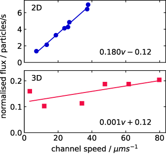
Figure 5. The normalised particle flux vs average particle speed within the channel for 2D (top) and 3D (bottom) geometry. The normalised flux (or capture rate) is defined as the number of particles entering the channel per second divided by the bulk packing fraction. Linear regression lines have been added to aid the eye, and the equations of those lines indicated in each panel.
Download figure:
Standard image High-resolution imageIf there were no driving force present (v = 0), we would expect no net particle flux through the channel, since the diffusive fluxes from each reservoir would be equal and opposite. As can be seen in figure 5, the 2D data would not be inconsistent with a fit through the origin, but this is clearly not the case for the 3D geometry. This suggests that for the 2D geometry we are in flow driven capture regime, and in 3D a diffusion-to-capture regime. In the former, the capture rate is proportional to flow speed, whereas in the latter the particle motion in the reservoirs is diffusive and therefore largely unaffected by channel flow speed. As long as the flow speed is large enough that the channel entrance can be considered an absorbing boundary ( m s−1), the capture rate is determined by the rate at which particles diffuse to that boundary. The exact location and shape of this boundary (the capture radius) will likely depend on flow speed, and can be investigated by considering the time-averaged particle concentration in the system.
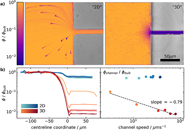
As such, in figure 6(a) we show the spatial variation of the concentration field away from the channel entrance. In each case, the local normalised concentration is defined as the packing fraction at a certain position normalised by its value far from the channel entrance in the reservoirs. Note that the darker features (or 'shadows') in the 2D data arise from a very small number of stuck particles in the sample. Figure 6(a) shows a more striking, qualitative difference in behaviour when compared to the velocity fields. In particular for this example, the 2D system shows a concentration reduction of a factor of 2 when moving from the reservoir to the channel, but for the 3D system, the concentration in the channel is a factor of approximately 100 less than in the reservoirs. This effect can be seen more clearly in figure 6(b) which shows the packing fraction along the centre line of the channel normalised as by the bulk packing fraction,  , for both the 2D and 3D geometries at a variety of different flow speeds.
Figure 6. The particle concentration field around the channel entrance for different chip geometries. (a) The spatial concentration field, normalised by the bulk packing fraction φbulk . The left panel shows the 2D case, and is an average over ∼98 000 frames of data. The right panel is the 3D case with ∼115 000 frames. 'Shadows' from a very small number of stuck particles are visible in the 2D geometry. (b) The normalised particle concentration along the channel axis for a number of different pressure differences. The left panel shows the normalised concentration as a function of distance, with the lines coloured according to the particle speed in the channel. x = 0 corresponds to the channel entrance. The right panel shows the fractional difference in concentration between the bulk and reservoir as a function of speed, with the points coloured corresponding to the lines in the left panel. For the 3D geometry, a linear regression line has been plotted and the slope indicated.
Download figure:
Standard image High-resolution image
It can be seen in figure 6(b), that the reduction in concentration for the channels in the 2D case is consistent and independent of flow speed. The origin of this reduction is currently unclear. As stated above, the particles lag the fluid flow by some fraction κ in all parts of the system. If we neglect particle interactions and assume the particles follow the streamlines of the fluid with κ constant in all parts of the system, then we would not expect a change in concentration in the channel. The fact that we observe a reduction in concentration could imply that the particles lag the fluid by a greater amount in the bulk than the channel, i.e.  , as from number conservation considerations, this would lead to a rarefaction. Alternatively, the reduction in concentration could be due to excluded volume effects, for example, particles being pushed into the faster streamlines in the centre of the channel.
In the 3D geometry, it is expected that the particles would be rarefied in the channel as the increase in vertical confinement causes the particles to experience disproportionately increased fluid flow as they approach the channel. Once the particles are caught in the faster flow they are transported much more quickly with respect to their velocity in the reservoir. As this is a flow based effect, we would expect to see a dependence of the rarefaction on flow speed and this is shown in figure 6(b). Empirically, we find that the rarefaction appears to follow a power law relationship  , however, currently the origins of this scaling are unclear: a theoretical model would have to account for the particles perturbing the fluid flow, as well as particle-particle interactions in the reservoir, and is beyond the scope of this work.
In conclusion, we have investigated the capture properties of colloids into microfluidic channels under pressure driven fluid flow. We have compared the behaviour in a '2D' geometry, where the entire microfluidic chip has the same depth, and a '3D' geometry, where the reservoirs are significantly deeper than the channels. In each case the particles lie in a single plane. We found that the 2D geometry shows longer range flow fields and attraction to the pore, with a consistent reduction in particle concentration within the channel of ∼50%. In contrast, the 3D geometry shows diffusion to capture behaviour, with high speeds within the channel but low particle fluxes, the particle concentration in the reservoir is observed to scale with  , a striking difference to the 2D case. Comparisons of the particle velocity fields within these geometries with fluid flow fields computed in the absence of particles suggest that at the packing fraction considered here (
 10%) particle-particle interactions do not significantly affect the transport behaviour. Our results provide insight on the design nuances of flow-based microfluidics, which are ubiquitous in medical devices and other 'lab-on-a-chip' measurement devices, and provide important experimental insight into the long-debated concept of the capture radius. Additionally, they demonstrate that optically imaged colloidal systems provide a versatile platform for investigating capture behaviour in a range of systems. We plan in future works to more deeply probe the nature of the capture radius and its dependence on both driving force and particle concentration, and to further probe parameter space with a view to an even higher degree of control over the capture properties of such systems.
Acknowledgments
The authors thank John Sherwood for helpful discussions. S F K acknowledges funding from UK Research and Innovation—Engineering and Physical Sciences Research Council (UKRI, EPSRC) and the EPSRC CDT in Nanoscience and Nanotechnology (NanoDTC). M F acknowledges support from the UK's Engineering and Physical Sciences Research Council Doctoral Training Programme and a Cambridge-NPL case studentship. J M H acknowledges funding from AFOSR (Grant No. FA9550-17-1-0118). A L T acknowledges support from the University of Cambridge Ernest Oppenheimer Fund and a Royal Society University Research Fellowship.
Data availability statement
The data that support the findings of this study are available upon reasonable request from the authors.