
Abstract
This work proposes a complete and consistent set of cross sections (CSs) for electron collisions with water molecules to be published in the IST-Lisbon database on LXCat. The set is validated from the comparison between experimental and computed electron swarm parameters. The former are collected from literature while the latter are calculated using a space-homogeneous two-term Boltzmann solver, assuming isotropic scattering in inelastic collisions. Rotational CSs, based on the Born approximation, are optimised by means of the electron swarm analysis technique. Superelastic rotational and vibrational collisions are accounted for in the calculations and found to be particularly important for low-energy electrons interacting with water molecules. The set can be used with codes assuming space-homogeneous conditions, in particular common two-term Boltzmann solvers, ensuring a good agreement with experiments. Therefore, it constitutes an important tool for fast calculations and modelling of complex plasma chemistries.
Export citation and abstract BibTeX RIS

Original content from this work may be used under the terms of the Creative Commons Attribution 4.0 license. Any further distribution of this work must maintain attribution to the author(s) and the title of the work, journal citation and DOI.
1. Introduction
An accurate characterisation of the interaction of water molecules and electrons is required in various fields of ongoing fundamental and application-oriented research. For instance, their interaction is relevant in plasma-in-liquid [1], waste (-water) and wound treatment with plasma [2, 3], or because water is an omnipresent impurity in atmospheric plasma [4], spark-ignited combustion [5], plasma sterilisation [6] and CO2 plasma conversion [7]. In these environments, electrons constitute the primary energy source to the heavy particles. Therefore, an accurate description of the electrons facilitates the understanding, tailoring and optimisation of water-containing discharges.
Electron-neutral collision cross sections (CSs), as provided here, are key to that description as they allow the calculation of the electron energy distribution function (EEDF) from the electron Boltzmann equation. A wide-spread solution approach is the use of two-term, space-homogeneous Boltzmann solvers such as LoKI-B [8] or BOLSIG+ [9].
Despite the clear demand, to this point there is no commonly agreed-on comprehensive CS set available for water neither on LXCat [10], i.e. one of the most extensive open-access CS websites, nor elsewhere, although many authors have proposed different sets either derived from experiments or ab-initio calculations [11–25]. A set's comprehensiveness is defined by two requirements, namely completeness and consistency. A complete set for H2O includes CSs for elastic, rotational, vibrational, electronic excitation, dissociation, ionisation and electron attachment collisions. When striving for the CSs, some studies [11, 13, 16] present valuable compilations of CSs, e.g. the recent extensive review by Song et al [16] but neglect the second requirement to a CS set that is consistency. A CS set must be validated against measurements [15, 17, 18, 26]. The macroscopic parameters derived from the solution of the Boltzmann equation, using the CS set presented here, are hence validated against experimental electron swarm parameters. Eventually, a complete and consistent set is obtained that is immediately usable for everybody due to the optimisation by means of the openly accessible two-term Boltzmann solver LoKI-B v2.1.0 [8].
The optimisation of swarm calculations for H2O is particularly challenging due to the variety and number of elementary processes involved, and attention must be paid to the assumptions taken prior to the optimisation of the CSs. For this reason, we decided to split the study into two contributions. In this work, we present a complete and consistent set of CSs that is derived under the assumptions of (i) two-term solutions of the electron Boltzmann equation, (ii) isotropic scattering in inelastic collisions, and (iii) equal energy sharing between scattered and secondary electrons in ionisation events. The assumptions come with well-known limitations like the restriction to small reduced electric fields, i.e. small anisotropy [27]. In a forthcoming second paper, we intend to evaluate these assumptions, e.g. through inclusion of anisotropy, and compare two-term Boltzmann solver calculations with multi-term and Monte Carlo simulations.
Probably the main reason for the ongoing discussion of H2O CSs is molecular rotations. Even though there is consensus in the community about the importance of rotations, especially for collisions with low-energy electrons, they are often not included properly in the CS sets. For instance on LXCat [10], at the time of writing this manuscript, some databases do not include rotations [12, 28, 29] or only provide lumped CSs (three in [30] and one in [31] in total). Other studies offer detailed rotational CSs but either the CSs or the used software are not openly accessible [15, 17]. Although CS and program should be independent, verification is impeded in these situations.
Henceforth, the objective of our work is clear, namely to provide a complete and consistent CS set for electron collisions with water molecules considering the most recent CSs and swarm data, including rotational collisions, to be used in an openly available standard two-term solver. The anticipated open-access release in the IST-Lisbon database [32] on LXCat gives the community the tools to include water in their plasma chemistry models.
2. Molecular quantum state of water
This section introduces to rotations of water molecules, required to treat rotational collisions with electrons. First, the rotational quantum state is characterised, second, peculiarities in the populations of rotational levels and transitions between them are discussed.
Inclusion of rotational collisions requires the proper characterisation of rotational states as presented in the following. The rotational state is denoted as J. The H2O molecule is an asymmetric-top rotor, i.e. it has three different finite moments of inertia which makes the description of the rotational state more complex than for a linear molecule like CO [33, 34]. In consequence, in addition to the principal rotational quantum number J (not to be confused with the notation of the rotational state itself J), two more quantum numbers are required. These are Kʹ and Kʹʹ, the projection of J along the axis of the smallest and largest moment of inertia, respectively. As of now, the rotational state is given by the three numbers J =  .
.
Next, we need to understand which rotational transitions to consider and how. Depending on the nuclear spin orientation of the two hydrogen atoms of the molecule, water is divided in two sets of spin isomers with different properties and nearly no interaction between the two. The pseudo-quantum number  is introduced [33], allowing to distinguish ortho-water (parallel nuclear spins) with odd τ and para-water (antiparallel nuclear spins) with even τ. Rotational transitions are only allowed within a set. At the same time, the statistical weight of a rotational state and thereby its population depends on the type of isomer of water [35]. The statistical weight is

Here, J is again the principal rotational quantum number,  the state-dependent nuclear spin statistical weight as a function of τ which is 1 for para- and 3 for ortho-water, respectively, and
  the state-independent nuclear spin statistical weight which is 1 for the most abundant water isotopologues [36]. A Matlab function to calculate
  to determine the level populations following a Boltzmann distribution at gas temperature, and the level energies required for that purpose are provided as supplementary material, see table 3 [37].
Finally, superelastic collisions are not only considered between rotational but also between vibrational states, indicated here as v. As a three-atomic molecule, water has three vibrational modes: (i) the symmetric stretching v1, (ii) the bending v2 and (iii) the asymmetric stretching v3. Thus, the vibrational state is characterised as v =  . Herein, a Boltzmann population distribution at gas temperature is assumed for the vibrational levels as well. The vibrational levels included in this set are indicated in table 1.
Table 1. Vibrational energy levels of water included in this work, vibrational energy with respect to the ground state and populations for a Boltzmann distribution at 293 K (given with the maximum accuracy accepted by BOLSIG+) [30].

| Energy (eV) | Population |
|---|---|---|
| 000 | 0.0 | 0.99961 |
| 010 | 0.198 | 0.00039 |
| 100 + 001 | 0.453 | 0.00000 |
3. The CS set
In this section, we present a throughout review of the CSs available in literature that are used as basis to construct our set. Furthermore, we present the final set of CSs that has been derived with the swarm analysis technique. In total, 163 CSs are considered.
Figure 1 shows the proposed CSs σ, plotted against the electron energy ε, divided into conservative collisions on the left with constant electron number and non-conservative processes, i.e. attachment and ionisation, on the right where the number of electrons changes. Among the available elastic CSs [12, 16, 30, 38] the one hard coded in the code Magboltz v11.9 by Biagi [38] gives the best immediate agreement with experimental swarm parameters. The solid black line in figure 1 represents this elastic CS after slight modification. As shown in figure 2, the high-energy tail of the elastic CS has been slightly decreased compared with the original CS, to better reproduce measurements of electron swarm parameters. Note the Ramsauer minimum at about 2.5 eV followed by a resonance [17] both customary well handled by LoKI-B [34].
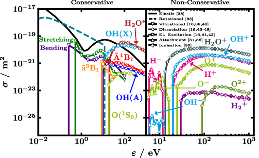
Figure 1. Proposed CSs σ, plotted against the electron energy ε, divided into conservative and non-conservative collisional processes without and with change in the number of electrons during the collision, respectively. The plotted rotational CS (dashed line) is the sum of all individual rotational CSs weighted by the populations of the lower rotational levels at 293 K. In the left-side panel, the elastic and rotational CS extend down to sub-meV range which is not shown for better visibility of the remaining conservative collision CSs. Original references of the CSs are given in the legend [16, 30, 31, 33, 38–46]. For a detailed record see table 2.
Download figure:
Standard image High-resolution image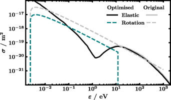
Figure 2. Comparison of optimised CSs σ, as proposed in figure 1, with the original unmodified CSs as taken from literature [33, 38] in grey plotted against the electron energy ε. For illustration, the rotational CS of transition  is arbitrarily chosen.
Download figure:
Standard image High-resolution imageTable 2. List of processes included in the proposed CS set.
| # | Process | Product | Threshold (eV) | Reference |
|---|---|---|---|---|
| 1 | Elastic | H2O | [38] | |
| 2 | Rotational | H2O(X,v = 000, J = 110) | 0.00230 | [33] |

|

| |||
| 148 | Rotational | H2O(X,v = 000, J = 551) | 0.03663 | [33] |
| 149 | Vibrational | H2O(X,v = 010) | 0.198 | [16, 39, 40] |
| 150 | Vibrational | H2O(X,v = 100 + 001) | 0.453 | [16, 39, 40] |
| 151 | Electronic Excitation | H2O( B1) B1) | 7.49 | [16, 41, 42] |
| 152 | Electronic Excitation | H2O( B1) B1) | 7.14 | [16, 41] |
| 153 | Dissociation | OH(X) + H(X) | 6.6 | [43] |
| 154 | Dissociation | OH(A) + H(X) | 9.2 | [44] |
| 155 | Dissociation | O(1S0) + 2H(X) | 13.696 | [16, 45] |
| 155 | Dissociation | H2O* | 18.0 | [46] |
| 156 | Attachment | OH−(X) + H(X) | 5.9 | [38] |
| 157 | Attachment | O−(X) + H2(X) | 4.9 | [31] |
| 158 | Attachment | H−(X) + OH(X) | 5.7 | [31] |
| 159 | Ionisation | H2O+ | 13.5 | [30] |
| 160 | Ionisation | H+(X) + OH(X) | 18.116 | [30] |
| 161 | Ionisation | H2(X) + O+(X) | 19.0 | [30] |
| 162 | Ionisation | H (X) + O(X) (X) + O(X) | 20.7 | [30] |
| 163 | Ionisation | H2(X) + O2+(X) | 80.0 | [30] |
The sum of the rotational CSs, each calculated according to Itikawa assuming the Born approximation [33] and weighted by the population of the initial rotational level at 293 K, is plotted as dashed line. It must be stressed that the sum is for illustration only, that is, in the actual calculation of the EEDF 147 individual rotational CSs are used. The Born approximation neglects short-range effects close to the threshold [19, 20]. Corrections due to the polar nature of the molecule, usually addressed by the Born-closure technique [13, 16, 20, 30], are not included neither beforehand nor implicitly by the code. Furthermore, we assume isotropic scattering which is why a forward angular discrimination correction [47] is not implemented. Arguments in favour of the Born approximation [48–50] and the obtained agreement with experiments in section 4 speak for the validity of the introduced simplifications. The lowest rotational level included is H2O(X,v = 000, J = 000) at 0 eV (reference value where X refers to the electronic ground state) while the highest level is H2O(X,v = 000, J = 660) at 0.12958 eV (given with the maximum accuracy accepted by BOLSIG+, like in table 1). This selection is in accord with the availability of line strength data from King et al [51] that is required for the calculation of the CSs. To better reproduce experimental measurements of electron swarm parameters, the rotational CSs derived from the Born approximation, are modified, under the assumption of isotropic electron scattering in the collisions. First, they are all scaled down by a factor of 0.3. Similarly, Song et al multiplied rotational NO CSs by 0.3 [52] or Kawaguchi et al scaled down rotational CSs of H2O by one order of magnitude [14]. The rotational CSs are then set to zero for electron energies larger than 12 eV, see figure 2 for illustration. Cutting the CSs at high energies leads to a better agreement with the reduced Townsend coefficient in figure 3. The importance of rotations is highlighted in figure 4 that shows the EEDFs of water with (dash-dotted lines) and without (solid lines) the 147 rotational CSs. Especially, at low reduced electric field of 10 Td a large difference between the two calculations is observed because at that  many electrons have low energy corresponding to large rotational CSs, despite the low energy losses in rotational collisions. The effect of rotations decreases with increasing reduced electric field due to the decreasing fraction of low-energy electrons, together with an increase of importance of higher energy losses.
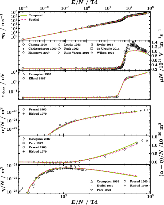
Figure 3. Comparison of experimental swarm parameters, when known with error bars, with those obtained from the LoKI-B simulation with the proposed CS set using either temporal (solid green line) or spatial growth (dotted magenta line) of the electron number [8]. Pay attention to (i) the linear y-axis scaling for panels with the y-label on the right-hand side, i.e. reduced mobility and reduced effective Townsend coefficient, and (ii) the smaller  range shown in the bottom three panels with respect to the top three. References to the experimental swarm parameters (markers) can be found in the text.
Download figure:
Standard image High-resolution image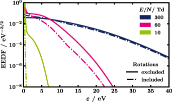
Figure 4. EEDFs of water calculated with LoKI-B [8] using the CS set proposed in figure 1 either including all 147 rotational transitions (dash-dotted lines) or completely excluding rotations (solid lines) for three different reduced electric fields  , namely 300, 60 and 10 Td in blue, magenta and green, respectively. Due to the increasing fraction of low-energy electrons, i.e. for which the rotational CSs are very large, with decreasing
  the difference between the solid and the dash-dotted lines increases.
Download figure:
Standard image High-resolution imageCollisional excitations from the vibrational ground state to the first vibrationally excited levels are included, see table 1. Due to the proximity of the thresholds of the stretching modes, they are not experimentally distinguishable and are described by a single CS. In literature, notations of 100 + 001 or 101 are found. Both vibrational CSs ( ), i.e. bending and stretching, are taken from Song et al [16], who in turn propose a combination of CS measured by Seng and Linder and Khakoo et al [39, 40].
The starting point for the excitation CSs for electronic states  B1 and
  B1 (
B1 ( ) are the CSs from measurements by Ralphs et al and Matsui et al [41, 42] as proposed by Song et al [16]. Both CSs are decreased by 10%, within the reported error margin, to obtain an agreement between calculated and measured electron swarm parameters. Additionally, multiple dissociation processes are included (
 ). The production of hydroxyl radicals in the electronic ground state OH(X) and the excited state OH(A) is represented by CSs from Harb et al and Beenakker et al [43, 44]. Both are also recommended by Biagi [38]. The production of O(1S0) is included by a CS from Kedzierski et al, increased by 30%, within the reported error margin, to improve the agreement with swarm parameters [45]. Finally, a CS is introduced to improve the agreement of the simulation with experiments for high reduced electric fields, denoted as H2O* on the left-hand side of figure 1 and plotted as
  like all electronic excitation processes. It is based on a CS by Möhlmann and de Heer for production of Balmer 3-2 emission, scaled up by a factor of 100. A similar treatment is adapted by Kawaguchi et al [14]. All modifications beyond a simple scaling by a constant factor can be comprehended from figure 2 that shows the original CSs, i.e. as taken from the [33, 38], in grey and the eventually proposed optimised CSs in the same colour as in figure 1.
The right-hand side of figure 1 displays the non-conservative processes. Three dissociative attachment CSs ( ) lead to the production of H−, O− and OH−, respectively. The former two are taken from the Triniti database on LXCat [10, 31] while the latter is taken from Biagi's Magboltz v11.9 [38]. Apart from the production of H2O+ also the ionisation processes are dissociative and result in OH+, H+, O+, O2+ and H
 , respectively. All ionisation CSs (
 ) are taken from the Itikawa database on LXCat [10, 30]. The production of O2+ is treated like a single-ionisation event yielding one secondary electron in the electron growth model (temporal growth with equal energy sharing, see section 4). Since only a small fraction (
 ) of the power deposited in total ionisation ends up in that particular ionisation channel, the error introduced by this simplified treatment is negligible.
All CSs in the set are summarised in table 2. A detailed list of the rotational transitions with thresholds and populations of the lower level can be found in the
4. Validation
The complete CS set presented in the previous section is validated by demonstrating that results obtained from a two-term Boltzmann solver are consistent with experimentally obtained electron swarm parameters from literature. Unless mentioned otherwise, all calculations in this paper are performed with the open-source code LoKI-B [8] to first obtain the general EEDF and then determine the swarm parameters from it. The required instructions, and setup as well as other input files are provided as supplementary material, see section
The electron swarm parameters are the electron drift velocity  [26, 53–61], the reduced mobility
  [53], the characteristic energy
  [62, 63], the reduced Townsend coefficient
  [64, 65], the reduced attachment coefficient
  [62, 64–67] and the reduced effective Townsend coefficient, defined as the difference of the latter two [54, 64, 65, 65]. Here, N is the total gas number density, µ the electron mobility,
  the transverse diffusion coefficient, α the Townsend coefficient and η the attachment coefficient. When not given explicitly, the reduced mobility is calculated from
  with E being the electric field and
  the reduced electric field, usually given in Townsend (
 V m2). Swarm parameters for water are provided in a relatively narrow temperature range. The two extremes, namely the study by Bailey and Duncanson at 288 K and the one by Pack, Voshall, and Phelps at 400 K, do not appear to agree with the other studies [26, 53–55, 57–60] and, as a consequence, are discarded here [56, 61]. The remaining studies report measurements at room temperature, i.e. between 290 to 300 K, and the gas temperature in the calculations is set to 293 K accordingly. All swarm parameters extracted from literature will be made available in the IST-Lisbon database on LXCat together with the proposed CS set.
Figure 3 shows the comparison of the calculated swarm parameters (lines) with the experimentally determined ones (markers). Note that the reduced mobility and the reduced effective Townsend coefficient (both with y-axis labels on the right) are plotted linearly while all other parameters are presented in logarithmic scale. Whenever known, the uncertainty of the experimental swarm parameters is shown as error bars. From top to bottom of figure 3,  ,
,  ,
,  ,
,  ,
,  and
and  are shown. The bottom three panels display only the high reduced electric field range since non-conservative processes are only relevant there, due to the high thresholds of the corresponding CSs, compare figure 1. Temporal (solid green line) as well as spatial growth (dotted magenta line) of the electron number is tested [8]. The former is the default throughout this paper.
The most significant feature of the swarm parameters of water, namely a very steep increase between 30 to 80 Td, is best observed for the reduced mobility  . As pointed out by Ness and Robson [15], this is due to the rapidly decreasing elastic CS, see figure 1. They show that, with a few simplifications, even a singularity would occur that is damped by vibrations, electronic excitations etc that dissipate the electron energy. In figure 4, the EEDFs of water, as calculated with LoKI-B, before (10 Td), during (60 Td) and after the strong increase (300 Td) are shown to illustrate the differences. Note that in any case the EEDF is strongly non-Maxwellian.
Even though the experimental swarm parameters are quite consistent, there is still some spread of data. For instance, the increase in  for decreasing
  measured by Kuffel (
 ) in the last panel of figure 3 [66], that was originally interpreted as consequence of three-body processes, is probably rather caused by impurities [67]. The measurements of Prasad and Craggs (
 ) [65] for the reduced Townsend and attachment coefficient, deviate from other references. Especially, their
  values could not be obtained with the available CSs and should be considered with care.
Additionally, the growth (model) of the electron number influences the outcome of simulations and measurements, as can be seen from the solid green and the dashed magenta line in figure 3. Usual configurations are pulsed Townsend (PT) and steady-state Townsend (SST) experiments, where the number of electrons grows, due to ionisation dominating over attachment, in time or in space, respectively [8, 27].  and
and  are determined from SST experiments, while
  (and thereby µ) and
  are determined from PT experiments. Simulations should consider the proper growth model, depending on which experimental values they try to reproduce [17, 68]. The set is optimised assuming temporal growth in the calculations with LoKI-B. While this approach obviously reduces the amount of necessary simulation runs, it particularly facilitates the comparison with Monte Carlo codes that often (but not exclusively) follow the electrons in time rather than in space [27]. However, in the presented range of
  the differences compared with the spatial growth model are negligible. The used growth model as well as other settings of the calculation can be found in the provided input file in the supplementary material.
The overall agreement of the calculations with the experimental swarm parameters is very good. In particular, the low reduced electric field range, dominated by rotations, is represented excellently. The largest disagreement is found between 100 to 400 Td, especially for  (note however, the linear scale of the figure). The maximum deviation from the experimental swarm parameters reaches up to 30%. While being most certainly not negligible, as the mobility influences the electron density when coupling the Boltzmann solver to a chemistry module, the agreement with parameters like
  , that are expected to have an even larger effect on the chemistry, is excellent. We consider this a drawback of the presented isotropic set since the agreement with the anisotropic set is improved as will be shown in a follow-up publication. However, the latter set is not usable in most Boltzmann solvers, which is why the former is a legitimate and useful compromise. The importance of our proposed set for the community is emphasised by comparing with results from other available sets as shown in figure 6 in the
Wide-spread acceptance of the proposed CS set demands that its applicability is not limited to LoKI-B but in principle comprises any space-homogeneous isotropic code. Admittedly, a thorough check against any code is clearly out of the scope of this publication. Therefore, we only refer to BOLSIG+ v11/19 since it is probably the most widely established two-term Boltzmann solver [9]. Its agreement with LoKI-B for atomic gases is proven [8]. For molecular gases like water, with inclusion of rotations and superelastic collisions, it is desirable to confirm. Eventually, this underpins the general validity of the CS set in space-homogeneous codes beyond LoKI-B.
The CSs are structured such that they can be parsed by LoKI-B and BOLSIG+ and describe the same physics. Primarily, rotational and vibrational states are populated correctly with respect to the gas temperature and superelastic collisions between them are included. When using the provided input file, LoKI-B automatically handles those aspects. Vibrational populations are manually entered in BOLSIG+, see table 1 at 293 K. Rotational populations are correctly calculated by BOLSIG+ by means of energy and statistical weight of each lower and upper rotational state as given with the CSs. Hence, any remaining differences between LoKI-B and BOLSIG+ are attributed to numeric reasons.
Figure 5 illustrates the differences between LoKI-B (solid green line) and BOLSIG+ (dashed blue line) based on the reduced attachment coefficient  plotted against the reduced electric field
  when using all CSs from table 2, particularly all 147 rotational CSs, in both codes together with markers that represent experimental data [63–67]. A deviation up to 10% between the two codes is noticed. However, both obtained curves give reasonable agreement with the experimental data. Since all other swarm parameters show better agreement, we take the 10% as a maximum estimation of the numeric uncertainty. Despite BOLSIG+ not being open source, after some testing, we can attribute these discrepancies to the following reasons.
- (a)ExtrapolationBOLSIG+ by default extrapolates CSs beyond their upper energy limit according to
 while they are set to zero by LoKI-B. For better comparison either the extrapolation is disabled in BOLSIG+ or the CSs are manually extrapolated following the energy dependence before using them in LoKI-B. The latter option is tested and reveals only a minor influence of the extrapolation.
 - (b)Population normalisationBOLSIG+ applies the normalisation condition to each superelastic excitation, particularly vibrational, collisional process separately by means of bi-Maxwellian Boltzmann factors while LoKI-B normalises over the full vibrational manifold. The vibrational populations as in table 1 are entered manually in BOLSIG+ to mitigate the influence of the population normalisation. Tests prove the influence of the normalisation to be negligible at 293 K though.
- (c)Effective CSStrictly speaking, we do not know how BOLSIG+ calculates the effective CS. We expect it to rely on the sum of elastic momentum transfer and inelastic CSs weighted by the fractional populations which connects this point to point (ii) as BOLSIG+ treats rovibrational states as individual species. Thus, we must consider this a major difference between the codes that is not further quantifiable.
- (d)Energy axisThe number of cells used to probe the energy axis that is scaled automatically to the maximum electron energy for both codes might not resolve the very low-energy thresholds of the rotational CSs. Also, the way the axis is scaled might be different. To minimise this component, the same number of cells (2000) is used in both codes to obtain figure 5. In LoKI-B the EEDF is set to span ten to fifteen decade-falls. As shown in figure 7 in the
appendix , the number of cells used in LoKI-B significantly influences (and ) as well, which is why we suspect the energy discretisation to be the dominating aspect in the difference between LoKI-B and BOLSIG+.


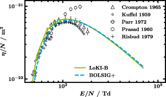
Figure 5. Comparison of the outcome of LoKI-B v2.1.0 and BOLSIG+ v11/19 for the same proposed isotropic set of CSs by means of the reduced attachment coefficient  against the reduced electric field
  . Markers represent experimental swarm parameters.
Download figure:
Standard image High-resolution imageThe points above only address differences between the codes. General advantages over one another, e.g. the more advanced physical models like magnetised plasma in BOLSIG+ [9] or the full consideration of the internal state of an atom or molecule in LoKI-B [8], are acknowledged. Nonetheless, they are of secondary importance here as the point to be made is the universal applicability of our CS set in space-homogeneous codes with different foci. We refer to the manuals of both codes for more details.
5. Conclusion
Even though water is a frequently encountered molecule in many innovative plasma applications, the community still lacks a commonly accessible, complete and consistent electron collision CS set with H2O which is required for the determination of the EEDF. While there is agreement on the significant influence of molecular rotations of water on the EEDF, particularly in the low-energy range, there is less consensus on how to include them. Here, we propose a CS set that addresses that predicament by optimising rotational CSs based on the Born approximation for dipole transitions by means of the electron swarm technique. Of the 163 CSs in the set 147 are rotational. The remaining CSs describe elastic, vibrational, electronic excitation, dissociation, attachment and ionisation collisions. The comparison of results of calculations with the two-term Boltzmann solver LoKI-B with experimental electron swarm parameters obtains good agreement, hence validating the proposed set. It allows simulations, performed with a common two-term solver, to consider water within reasonable calculation time and accuracy. Thereby, the set promotes the development of more sophisticated plasma chemistry models and consequently facilitates the understanding and optimisation of experiments and applications. The set will be made available to the community in the IST-Database on LXCat [32]. A future study will investigate the importance of anisotropy in scattering events.
Acknowledgments
The authors acknowledge the comments of Luís Lemos Alves, particularly regarding the use of BOLSIG+. This work was partially supported by the European Union's Horizon 2020 research and innovation programme under Grant Agreement MSCA ITN 813393, by Portuguese FCT-Fundação para a Ciência e a Tecnologia, under Projects UIDB/50010/2020, UIDP/50010/2020 and PTDC/FIS-PLA/1616/2021 (PARADiSE), Grant PD/BD/150414/2019 (PD-F APPLAuSE) and EXPL/FIS-PLA/0076/2021. L V acknowledges fundings from Deutsche Forschungsgemeinschaft (DFG, German Research Foundation)—Project-ID 434434223 - SFB 1461.
Data availability statement
All data that support the findings of this study are included within the article (and any supplementary files).
Appendix A.: Comparison with other databases
Even though there are published compilations of CSs that are certainly valuable options to pick from, these compilations are often not complete and consistent sets of CSs. To further motivate the need for our work presented here, in figure 6 the electron swarm parameters calculated from LoKI-B using our recommended set (solid green line), the CSs from Song et al [16] (dashed orange line) and the Itikawa database on LXCat [30] (dash-dotted blue line) are plotted against  together with experimental swarm parameters (markers). The former CS set is an update of the latter which is in turn based on [13]. The solid green line is the same as in figure 3.
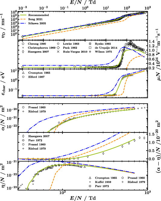
Figure 6. Comparison of experimental swarm parameters, when known with error bars, with those obtained from the LoKI-B simulation with the recommended CS set (solid green line), the one from Song et al [16] (dashed orange line) and the one from the Itikawa database on LXCat [30], originally based on Itikawa and Mason [13] (dash-dotted blue line). Pay attention to (i) the linear y-axis scaling for panels with the y-label on the right-hand side, i.e. reduced mobility and reduced effective Townsend coefficient, and (ii) the smaller  range shown in the bottom three panels with respect to the top three. References to the experimental swarm parameters (markers) can be found in the text.
Download figure:
Standard image High-resolution imageSong et al and the Itikawa database are chosen since they present relatively recent extensive compilations of H2O CSs both including rotations. Song et al provide in their supplementary material state-to-state rotational CSs  that only need to be transferred to LoKI-B/BOLSIG+-readable format. All other CSs are taken as is from the tables in the publication. On the other hand, the Itikawa database only includes lumped rotational CSs (
 ). As effective rotational energy levels the thresholds of the four transitions are used, as effective statistical weight
  is assumed. Finally, for both sets the given partial ionisation CSs are used, i.e. the total ionisation CS is removed.
It is immediately visible from figure 6 that in contrast to our recommended CS set neither Song et al nor Itikawa give a satisfying agreement with experimental swarm parameters. From the drift velocity in the first panel it appears that the Itikawa set gives reasonable agreement with experiments. However, a look at the second panel showing the reduced mobility calculated from  , i.e. principally the same data as in the first panel but in linear scale, reveals a strong disagreement also for Itikawa. For the reduced Townsend and attachment coefficient in the fourth and sixth panel a better agreement with experiments and the proposed CS set is observed for
  higher than 150 Td. Since the ionisation CSs in our set are taken from the Itikawa database [30], see table 2, and CSs from Song et al [16] exhibit only slight changes compared to Itikawa and Mason's CSs, this behaviour is expected. For the reduced effective Townsend coefficient in the fifth panel, i.e. the difference between
  and
and  , the opposite trend is observed with a better agreement of Itikawa and Song for low
  . We attribute this to two deviations cancelling each other, see the strong divergence from experimental values for
  and
and  below 150 Td. Note also the linear scale in that panel. Overall, the disagreement between experiments and calculations using CSs from Itikawa and Song is not surprising, as the purpose of their studies is different from ours. By means of a vast comparison of literature, they are able to give excellent individual CSs of water. We on the other hand focused on the entire set from the very beginning and optimised it accordingly by the electron swarm method to obtain the good agreement shown in figure 6, despite applied simplifications like rotational CSs calculated from the Born approximation.
Appendix B.: Influence of the energy discretisation
The difficulties mentioned in the main text regarding the choice of the number of cells that the electron energy axis is divided in, deserve some further discussion. Because the thresholds of the rotational transitions are very small, see for instance table 3, i.e. reaching down to the sub-meV range, they cannot be resolved by the minimum energy increment of commonly advised cell numbers. For instance, in the latest version of LoKI-B the default cell numbers are 1000 for Ar, CO, CO2, and He and 2000 for N2 and O2. Noticeable differences are observed when integrating over the EEDF to obtain the swarm parameters depending on the used number of cells.
This is illustrated in figure 7, where the deviation of the calculation results and the required calculation time are plotted against the used cell number. Apart from the cell number the settings are the same as in figure 5 which means the Boltzmann equation is solved for thirty values of  between 0.01 and 700 Td. Assuming the results get more and more accurate with increasing cell number, i.e. the results with 9000 cells are the best of the recorded sample, all other results are related to the latter. The deviation of the results per swarm parameter is represented by means of the average absolute percentage difference with respect to the outcome when using 9000 cells and hence the average deviation of 9000 cells is 0%. The lines in figure 7 are polynomial fits meant as guides to the eye. The dashed green line confirms the expected quadratic increase of calculation time with cell number (within performance variations of the used PC).
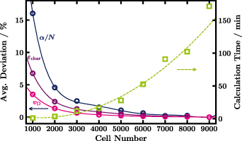
Figure 7. Percentage deviation of swarm parameters with respect to the results for 9000 cells (circles,left) and calculation time (squares,right) plotted against the used number of cells to discretise the energy axis in the calculation with LoKI-B. Lines are polynomial fits to the data to serve as guides to the eye.
Download figure:
Standard image High-resolution imageHigher resolution by an increased number of cells comes with the cost of increased calculation time. For instance, for LoKI-B we find the results to be independent of the number of cells, when at least 8000 cells are included in the calculations. However, the calculation time is then unfeasible for coupling to chemical kinetics. Therefore, we recommend 2000 cells to be used for the isotropic set. Reduced Townsend and attachment coefficient show the largest deviation (as they are more or less identical only the deviation for  is plotted) that is still less than 5% with respect to 9000 cells for the recommended number of cells, i.e. 2000.
Appendix C.: Rotational transitions
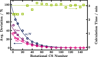
For completeness, all considered rotational transitions are given in table 3 ordered by the magnitude of the rotational CS weighted by the population of the lower state. Even though the large number of rotational transitions ensures the proper behaviour with changing temperature, from a fluid modelling point of view it is less desirable. To evaluate the compromise of reducing the number of transitions considered see figure 8. It turns out that the 80 largest rotational CS at 293 K still give almost the same swarm parameters. Afterwards large deviations are observed. The calculation time is mostly unaffected by the number of CS. We recommend to always use the total number of 147 rotational CS.
Figure 8. Percentage deviation of swarm parameters with respect to the results for 147 included rotational CSs (circles,left) and calculation time (squares,right) plotted against the used number of largest rotational CSs in the calculation with LoKI-B. Lines are fits to the data to serve as guides to the eye. 2000 cells are used.
Download figure:
Standard image High-resolution image
Table 3. Considered rotational transitions of water  J' with respective threshold taken from Tennyson et al and population of lower state assuming a Boltzmann distribution at 293 K [37]. Numbering as in table 2.
| # | J | Jʹ | Threshold (eV) | Population |
|---|---|---|---|---|
| 2 | 101 | 110 | 0.00230 | 0.01496 |
| 3 | 303 | 312 | 0.00454 | 0.02004 |
| 4 | 312 | 321 | 0.00481 | 0.01674 |
| 5 | 101 | 212 | 0.00691 | 0.01496 |
| 6 | 212 | 303 | 0.00710 | 0.01896 |
| 7 | 202 | 211 | 0.00311 | 0.00662 |
| 8 | 303 | 414 | 0.01092 | 0.02004 |
| 9 | 110 | 221 | 0.01147 | 0.01365 |
| 10 | 414 | 505 | 0.01246 | 0.01672 |
| 11 | 514 | 523 | 0.00583 | 0.00867 |
| 12 | 212 | 221 | 0.00687 | 0.01896 |
| 13 | 000 | 111 | 0.00460 | 0.00187 |
| 14 | 505 | 616 | 0.01512 | 0.01247 |
| 15 | 523 | 616 | 0.00009 | 0.00688 |
| 16 | 221 | 330 | 0.01866 | 0.01444 |
| 17 | 413 | 422 | 0.00499 | 0.00435 |
| 18 | 202 | 313 | 0.00895 | 0.00662 |
| 19 | 414 | 423 | 0.00936 | 0.01672 |
| 20 | 312 | 423 | 0.01575 | 0.01674 |
| 21 | 211 | 220 | 0.00508 | 0.00585 |
| 22 | 111 | 202 | 0.00409 | 0.00467 |
| 23 | 523 | 532 | 0.00773 | 0.00688 |
| 24 | 313 | 404 | 0.00989 | 0.00650 |
| 25 | 321 | 330 | 0.00908 | 0.01384 |
| 26 | 505 | 514 | 0.00919 | 0.01247 |
| 27 | 423 | 432 | 0.01019 | 0.01154 |
| 28 | 321 | 432 | 0.02112 | 0.01384 |
| 29 | 212 | 321 | 0.01645 | 0.01896 |
| 30 | 404 | 413 | 0.00663 | 0.00565 |
| 31 | 404 | 515 | 0.01297 | 0.00565 |
| 32 | 330 | 441 | 0.02513 | 0.00966 |
| 33 | 221 | 312 | 0.00477 | 0.01444 |
| 34 | 423 | 514 | 0.01229 | 0.01154 |
| 35 | 111 | 220 | 0.01228 | 0.00467 |
| 36 | 321 | 414 | 0.00157 | 0.01384 |
| 37 | 313 | 322 | 0.00794 | 0.00650 |
| 38 | 211 | 322 | 0.01378 | 0.00585 |
| 39 | 514 | 625 | 0.01903 | 0.00867 |
| 40 | 220 | 313 | 0.00076 | 0.00479 |
| 41 | 515 | 606 | 0.01489 | 0.00413 |
| 42 | 220 | 331 | 0.01848 | 0.00479 |
| 43 | 422 | 431 | 0.00844 | 0.00357 |
| 44 | 432 | 541 | 0.02825 | 0.00771 |
| 45 | 330 | 423 | 0.00185 | 0.00966 |
| 46 | 625 | 634 | 0.01191 | 0.00482 |
| 47 | 423 | 532 | 0.02585 | 0.01154 |
| 48 | 616 | 625 | 0.01310 | 0.00810 |
| 49 | 532 | 541 | 0.01259 | 0.00507 |
| 50 | 615 | 624 | 0.00742 | 0.00169 |
| 51 | 322 | 331 | 0.00979 | 0.00475 |
| 52 | 441 | 550 | 0.03149 | 0.00459 |
| 53 | 432 | 441 | 0.01309 | 0.00771 |
| 54 | 413 | 524 | 0.01745 | 0.00435 |
| 55 | 322 | 431 | 0.02201 | 0.00475 |
| 56 | 322 | 413 | 0.00858 | 0.00475 |
| 57 | 624 | 633 | 0.00729 | 0.00126 |
| 58 | 331 | 440 | 0.02516 | 0.00322 |
| 59 | 523 | 634 | 0.02511 | 0.00688 |
| 60 | 515 | 524 | 0.01111 | 0.00413 |
| 61 | 524 | 533 | 0.01088 | 0.00266 |
| 62 | 634 | 643 | 0.01336 | 0.00301 |
| 63 | 532 | 643 | 0.03074 | 0.00507 |
| 64 | 432 | 523 | 0.00794 | 0.00771 |
| 65 | 524 | 615 | 0.01571 | 0.00266 |
| 66 | 422 | 533 | 0.02333 | 0.00357 |
| 67 | 541 | 652 | 0.03450 | 0.00308 |
| 68 | 431 | 542 | 0.02806 | 0.00255 |
| 69 | 606 | 615 | 0.01193 | 0.00271 |
| 70 | 532 | 625 | 0.00547 | 0.00507 |
| 71 | 422 | 515 | 0.00134 | 0.00357 |
| 72 | 313 | 422 | 0.02151 | 0.00650 |
| 73 | 414 | 523 | 0.02749 | 0.01672 |
| 74 | 533 | 542 | 0.01316 | 0.00173 |
| 75 | 431 | 440 | 0.01293 | 0.00255 |
| 76 | 440 | 551 | 0.03149 | 0.00153 |
| 77 | 441 | 532 | 0.00257 | 0.00459 |
| 78 | 550 | 661 | 0.03757 | 0.00161 |
| 79 | 331 | 422 | 0.00379 | 0.00322 |
| 80 | 541 | 550 | 0.01633 | 0.00308 |
| 81 | 633 | 642 | 0.01193 | 0.00094 |
| 82 | 431 | 524 | 0.00401 | 0.00255 |
| 83 | 643 | 652 | 0.01635 | 0.00177 |
| 84 | 541 | 634 | 0.00479 | 0.00308 |
| 85 | 533 | 642 | 0.03147 | 0.00173 |
| 86 | 542 | 651 | 0.03454 | 0.00103 |
| 87 | 524 | 633 | 0.03042 | 0.00266 |
| 88 | 533 | 624 | 0.01225 | 0.00173 |
| 89 | 440 | 533 | 0.00196 | 0.00153 |
| 90 | 550 | 643 | 0.00182 | 0.00161 |
| 91 | 551 | 660 | 0.03757 | 0.00054 |
| 92 | 542 | 551 | 0.01636 | 0.00103 |
| 93 | 642 | 651 | 0.01623 | 0.00059 |
| 94 | 303 | 432 | 0.03047 | 0.02004 |
| 95 | 542 | 633 | 0.00638 | 0.00103 |
| 96 | 652 | 661 | 0.01940 | 0.00093 |
| 97 | 505 | 634 | 0.04013 | 0.01247 |
| 98 | 505 | 532 | 0.02275 | 0.01247 |
| 99 | 515 | 624 | 0.03424 | 0.00413 |
| 100 | 303 | 330 | 0.01843 | 0.02004 |
| 101 | 551 | 642 | 0.00195 | 0.00054 |
| 102 | 505 | 432 | 0.00709 | 0.01247 |
| 103 | 404 | 533 | 0.03496 | 0.00565 |
| 104 | 404 | 431 | 0.02006 | 0.00565 |
| 105 | 651 | 660 | 0.01940 | 0.00031 |
| 106 | 514 | 643 | 0.04430 | 0.00867 |
| 107 | 514 | 541 | 0.02615 | 0.00867 |
| 108 | 202 | 331 | 0.02668 | 0.00662 |
| 109 | 606 | 533 | 0.00710 | 0.00271 |
| 110 | 615 | 642 | 0.02664 | 0.00169 |
| 111 | 606 | 633 | 0.02664 | 0.00271 |
| 112 | 404 | 331 | 0.00783 | 0.00565 |
| 113 | 312 | 441 | 0.03903 | 0.01674 |
| 114 | 413 | 542 | 0.04149 | 0.00435 |
| 115 | 414 | 541 | 0.04780 | 0.01672 |
| 116 | 615 | 542 | 0.00833 | 0.00169 |
| 117 | 514 | 441 | 0.01099 | 0.00867 |
| 118 | 413 | 440 | 0.02637 | 0.00435 |
| 119 | 523 | 652 | 0.05482 | 0.00688 |
| 120 | 616 | 643 | 0.03837 | 0.00810 |
| 121 | 414 | 441 | 0.03264 | 0.01672 |
| 122 | 515 | 642 | 0.05346 | 0.00413 |
| 123 | 625 | 652 | 0.04162 | 0.00482 |
| 124 | 515 | 542 | 0.03515 | 0.00413 |
| 125 | 423 | 550 | 0.05477 | 0.01154 |
| 126 | 313 | 440 | 0.04288 | 0.00650 |
| 127 | 523 | 550 | 0.03665 | 0.00688 |
| 128 | 624 | 651 | 0.03545 | 0.00126 |
| 129 | 524 | 651 | 0.05858 | 0.00266 |
| 130 | 616 | 541 | 0.02022 | 0.00810 |
| 131 | 422 | 551 | 0.05286 | 0.00357 |
| 132 | 532 | 661 | 0.06649 | 0.00507 |
| 133 | 524 | 551 | 0.04041 | 0.00266 |
| 134 | 634 | 661 | 0.04911 | 0.00301 |
| 135 | 515 | 440 | 0.02003 | 0.00413 |
| 136 | 505 | 652 | 0.06984 | 0.01247 |
| 137 | 625 | 550 | 0.02346 | 0.00482 |
| 138 | 533 | 660 | 0.06709 | 0.00173 |
| 139 | 624 | 551 | 0.01727 | 0.00126 |
| 140 | 633 | 660 | 0.04755 | 0.00094 |
| 141 | 404 | 551 | 0.06448 | 0.00565 |
| 142 | 606 | 651 | 0.05480 | 0.00271 |
| 143 | 616 | 661 | 0.07413 | 0.00810 |
| 144 | 615 | 660 | 0.06227 | 0.00169 |
| 145 | 515 | 660 | 0.08908 | 0.00413 |
| 146 | 505 | 550 | 0.05167 | 0.01247 |
| 147 | 514 | 661 | 0.08005 | 0.00867 |
| 148 | 606 | 551 | 0.03663 | 0.00271 |
Appendix D.: Provided files and instructions
The following files are provided with this manuscript:
- rotationalDegeneracy_H2O.mA Matlab function to calculate the statistical weight of rotational levels of water under consideration of the differences between ortho- and para-water. The function is easily coupled to the open-source code LoKI-B where it is used in the input file (provided as well) by means of statisticalWeight: - H2O(X,v = 000,J = *) = rotationalDegeneracy_H2O ... but can also serve as stand-alone function.
- rotEnergy_Tennyson.txtA Text file containing a two-column table with the rotational state in the first and its corresponding energy in the second column. It is needed for the calculation of the rotational populations in LoKI-B by the line energy: - Water/H2O_rotEnergy_Tennyson.txt ... in the input file (assuming all the energy files to be contained in the input subfolder Water).
- vibEnergy_Itikawa.txtAnother Text file that gives the same data for the vibrational levels energy: - Water/H2O_vibEnergy_Itikawa.txt ...
- H2O_swarm_setup.inThe input file used to control the calculations by LoKI-B. We refer to [8] for details on the usage. In the optimisation 2000 cells, equal energy sharing between primary and secondary electrons and temporal electron number growth are used.
Supplementary data (<0.1 MB TXT) Rotational energy levels of H2O
Supplementary data (<0.1 MB IN) Default input file for H2O in LoKI-B
Supplementary data (<0.1 MB TXT) Vibrational energy levels of H2O
Supplementary data (<0.1 MB M) Rotational degeneracy of H2O