
Abstract
Strong-field ionization of atoms can be investigated on the attosecond time scale by using the attoclock method, i.e. by observing the peak of the photoelectron momentum distribution (PMD) after applying a laser pulse with a two-dimensional polarization form. Examples for such laser fields are close-to-circular or bicircular fields. Here, we report numerical solutions of the time-dependent Schrödinger equation for bicircular fields and a comparison with a compact classical model to demonstrate that the tunnel-exit position, i.e. the position where the electron emerges after tunnel ionization, is encoded in the PMD. We find that the tunnel-exit position depends on the transverse velocity of the tunneling electron. This gives rise to a momentum-dependent attoclock shift, meaning that the momentum shift due to the Coulomb force on the outgoing electron depends on which slice of the momentum distribution is analysed. Our finding is supported by a momentum-space-based implementation of the classical backpropagation method.
Export citation and abstract BibTeX RIS

Original content from this work may be used under the terms of the Creative Commons Attribution 4.0 licence. Any further distribution of this work must maintain attribution to the author(s) and the title of the work, journal citation and DOI.
1. Introduction
Resolving the ionization process in ultrashort intense laser pulses on the attosecond time scale and the angstrom length scale is a key challenge in the investigation of strong-field above-threshold ionization (ATI). Its detailed understanding is of high importance as the ionization step creates electron wave packets in the continuum that can afterwards induce processes such as high-harmonic generation [1–6], laser-induced electron diffraction [7–12] and strong-field photoelectron holography [13–17]. Since these phenomena are often interpreted by means of trajectory-based models [18–22], precise information on the initial conditions of the electron after its release from the parent ion is advantageous.
Attosecond angular streaking, also known as the 'attoclock' technique, offers a possibility to probe the ionization process. In many implementations [23–26] close-to-circularly polarized laser fields have been used to ionize atoms. Neglecting the influence of the long-range binding potential on the outgoing electron, the simple man's model [27] predicts that the maximum of the photoelectron momentum distribution (PMD) coincides with the negative vector potential −A(tpeak) at the time tpeak of peak electric-field strength (atomic units are used unless stated otherwise) 3 . However, in the experiment, or when solving the time-dependent Schrödinger equation (TDSE) [30], there is a measurable angular offset between the actual maximum of the PMD and −A(tpeak). This offset is termed global attoclock shift. To retrieve characteristic features of the ionization process such as the ionization time [23] or the initial position [25] from the offset angle, theoretical models are needed. Even though models make additional assumptions beyond the plain quantum-mechanical theory, they often facilitate the understanding of physical mechanisms, provided they can reproduce the correct results. In a trajectory-based picture, the electron is first released by, e.g. tunnel ionization and afterwards accelerated by the laser electric field as well as the Coulomb field of the parent ion such that the initial conditions (ionization time, velocity and position) are mapped to final electron momenta. Recent theoretical investigations using various techniques such as the analytical R-matrix theory [28], the classical backpropagation method [31–33], classical trajectory Monte-Carlo simulations [34], trajectory-free ionization times from Dyson integrals [35] and a classical Rutherford scattering model [36] have shown that deviations from the simple man's model are mostly related to the Coulomb field of the residual ion. Since this interaction depends strongly on the initial position (tunnel exit) of the electron, the attoclock can be used as a fine 'nano-ruler' that measures the width of the tunnel barrier [37]. In the following, the tunnel-barrier width is identified with the tunnel-exit position (thereby neglecting that the tunnel entrance is not exactly at the origin). A summary of the various developments in attoclock-like setups and their interpretation can be found in references [37, 38].
Previously, it has been shown that the attoclock offset depends on the momentum of the electron in the polarization plane [29]. The aim of this paper is to show that the momentum-dependent attoclock offset is strongly influenced by the tunnel-exit position which in turn depends on the initial velocity of the electron. To this end, we introduce an adiabatic trajectory model that reproduces the results from the numerical solution of the TDSE. Since non-adiabatic effects [39, 40] as well as geometrical effects in the momentum-dependent analysis complicate the interpretation in close-to-circularly polarized fields, it would be beneficial to study the dynamics in linear polarization. However, in purely linearly polarized fields the part of the PMD that corresponds to ionization at peak electric-field strength is centered around zero momentum and thus strongly influenced by Coulomb effects [41, 42]. Additionally, the occurrence of sub-cycle interferences [43, 44] spoils the signal from a single ionization time. To avoid these problems, we study the strong-field dynamics in an alternative waveform: a bicircular ω–2ω field composed of two counter-rotating components [45–51] can be tailored such that the electric field approximates linear polarization three times per optical cycle of the fundamental component, while providing a time-to-momentum mapping similar to the conventional attoclock [29, 52]. We refer to this field geometry as a quasi-linear electric field. For this particular 'bicircular attoclock', the Coulomb effect leads to a shift of the electron momentum distribution along the direction of the instantaneous electric field [29]. In the vicinity of the electric field maxima, the setting is nearly isotropic in the directions perpendicular to the electric field (analogous to pure linear polarization). Hence, the bicircular field offers a clean setup to study the dependence of the attoclock shift on the initial velocity of the electron at the tunnel exit.
In the adiabatic regime, characterized by a small Keldysh parameter  , strong-field ionization can be described by tunneling through a potential barrier caused by the joint effect of the ionic core and the laser field. Here, Ip is the ionization potential of the atom, ω is the frequency of the laser field and E is its amplitude. In a stationary one-dimensional scenario, the tunnel-barrier exit is naturally defined by the zero-kinetic-energy principle [53]. However, in higher spatial dimensions and for a time-dependent tunnel barrier (non-zero Keldysh parameters) ambiguities arise due to the choice of the tunneling coordinate and because of a non-conserved energy during tunneling. Even under such conditions the classical backpropagation method [31–33] offers a possibility to determine characteristic features of the tunneling process, e.g. the relation between ionization time, initial velocity and tunnel-exit position, from an ab initio calculation. To this end, the ionization step is firstly treated fully quantum mechanically. Afterwards the ejected electron wave packet is transformed into a swarm of classical trajectories and propagated backwards in time until a tunneling criterion is met. Here, we find that the tunnel-exit positions obtained from backpropagation also depend on the initial velocity of the electron. This supports our model of the momentum-dependent attoclock shifts.
2. Methods
2.1. Numerical solution of the TDSE
We consider ionization of helium under the influence of a strong laser pulse with an electric field E(t) by using a single-active-electron (SAE) description in dipole approximation. The SAE description approximates the relevant electron dynamics in attoclock-like experiments with helium very well [54], compare also the reviews [37, 38]. To this end, the TDSE,

is solved in velocity gauge for a given vector potential  and a binding potential V(r). In 3D, the effective potential V for the helium atom is chosen as by Tong and Lin [55], but with the singularity removed using a pseudopotential for the 1s state with a cutoff radius rcl = 1.5 a.u. [56]. In order to reduce the numerical workload, we additionally study the dynamics in a 2D helium model. To this end, the potential is further softened by replacing
  such that the correct ionization potential Ip = 0.90 a.u. is obtained. The ground state (serving as initial state) is calculated as eigenstate of the short-time field-free time-evolution operator for a time step Δt = 0.02 a.u. as described in [57]. This method of finding the initial state is beneficial for obtaining reliable PMDs even in regions of low signal in momentum space.
We solve numerically the TDSE using the split-operator method on a Cartesian grid [58]. In 3D, we follow the scheme presented in [59] and divide the three-dimensional configuration space in an inner region and an asymptotic outer region. This approach is related to the mask method introduced in [60, 61]. The binding potential is fully included on the inner grid that spans 409.6 a.u. in each dimension with a spacing of Δx = 0.4 a.u. At the edge of the inner grid, the binding potential is turned off smoothly. In the asymptotic outer region the interaction of the electron with the ionic potential is neglected. Hence, this wave function is represented in momentum space at all times and it is propagated until a final time tf by means of Volkov states. The inner region has an absorbing boundary covering a distance of 50 a.u. from the edge of the grid. The absorbed parts of the inner wave function are not discarded, but added coherently to the wave function of the outer region. Thus, the momentum-space wave function  of the ionized system is collected in the outer region.
In 2D, we use the same method as in 3D (with a grid spanning 682.7 a.u. and using Δx = 0.17 a.u.) when the laser parameters are such that the vector potential A(0) is large. For sufficiently low vector potentials A(0), however, we choose a large inner grid spanning 4096 a.u. in each direction, which is enough to contain the wave function till the end of the laser pulse (at time tp). To obtain the momentum representation  of the outgoing photoelectron wave packet at a sufficiently large time tf ≫ tp, we remove the localized bound states with a mask function in the range r < 20 a.u. Afterwards the remaining part of the wave function ψ(r, tp) is further propagated using the eikonal approximation

with  . From the momentum-space wave function
  of the ionized wave packet the PMD is obtained as modulus square:
  . While the results from the 2D TDSE simulations are fully converged with respect to variation of the numerical parameters, the convergence is more difficult to assess for the time-consuming 3D results. In 3D, the numerical capabilities prevent us from further enlarging the used grids in position space. However, we have alternatively solved the TDSE with the generalized pseudospectral method [62, 63] and have calculated the PMD by projection on Coulomb waves. For the lowest intensity used, we have verified that the results from the two numerical methods are in very good agreement. We estimate the numerical error for the presented 3D results to be smaller than 10 percent.
2.2. Modified classical backpropagation
The essence of the classical backpropagation method is first to propagate fully quantum-mechanically the initial state forward in time by solving the TDSE till a final time tf [31–33]. Afterwards the liberated wave packet is transcribed to a classical phase-space distribution, which is then used as initial distribution for a swarm of classical trajectories evolving backwards in time. In previous implementations, e.g. [29, 31–33], the position-space quantum mechanical wave packet has been used to initiate the classical trajectories and the local-momentum method has been applied to assign a local momentum p(r) to each position r. Here, we follow a slightly different path and we use the momentum-space wave function  to initiate the classical backpropagation. To this end, we express the wave packet
 ![$~{\psi }(\mathbf{p},{t}_{\text{f}})=R(\mathbf{p},{t}_{\text{f}})\mathrm{exp}[\mathrm{i}S(\mathbf{p},{t}_{\text{f}})]$](https://content.cld.iop.org/journals/0953-4075/54/16/164001/revision2/bac190dieqn10.gif) by means of a real-valued amplitude and phase. For a given momentum p, the corresponding position is obtained by the 'local-position method'
by means of a real-valued amplitude and phase. For a given momentum p, the corresponding position is obtained by the 'local-position method'

Naturally, this method only works well when interference has a negligible effect on the final electron momentum distribution. For binding potentials with finite support and sufficiently long times tf, it can be shown that the obtained phase-space distribution is equivalent to the one from previous implementations based on the local-momentum method (see section 3.4 for further details).
To better understand the tunneling dynamics, we identify the exit point of the under-the-barrier motion by propagating the swarm of classical trajectories backward in time following Newton's equation. For each trajectory, the backpropagation is stopped at a time t0, when the velocity in the direction of the instantaneous electric field E(t0) vanishes (velocity criterion, see references [31, 32]). This results in an initial distribution wini(t0, v⊥, vz ) that can be parameterized by an ionization time t0, a velocity component in the polarization plane v⊥ and a velocity component in light propagation direction vz . The position of the electron at the ionization time t0 can be interpreted as tunnel-exit position. By construction, the quantum-mechanical momentum distribution at time tf is exactly reproduced by classical trajectories that are launched according to the distribution wini(t0, v⊥, vz ) at the velocity- and time-dependent tunnel-exit positions.
3. Results and discussion
3.1. Momentum-dependent attoclock shifts
An attoclock-like configuration with quasi-linear fields provides a clean setup to study the momentum dependence of the attoclock shift. To this end, we use a field consisting of a superposition of two counter-rotating circularly polarized fields with the following vector potential

For the particular field-strength ratio 2:1 of the fundamental to the second harmonic, the laser field is approximately linearly polarized near the peaks of the electric field [29]. In particular, around t = 0 we can write
Hence, the electric field resembles a linearly polarized field along the y-axis with an effective frequency  and a peak field strength Epeak related to the time-averaged intensity of the field by
  . The adiabaticity of the ionization process can be quantified by the Keldysh parameter
  . For numerical calculations, the vector potential of equation (4) is multiplied with an envelope f(t) = cos4(ωt/(2np)) of np cycles duration. To avoid the appearance of ATI rings in the relevant part of the momentum distribution, we use three- or five-cycle pulses. The characteristic shapes of vector potential and electric field are depicted in figure 1(a).
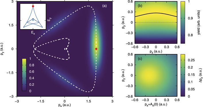
Figure 1. (a) 2D slice through the PMD w(p) at pz = 0 for ionization of helium by a three-cycle pulse with an effective wavelength of 800 nm and an intensity of 1015 W cm−2 (Epeak = 0.160 a.u.). The white dashed line shows the negative vector potential and the inset shows the electric field evolving in time. (b) Signal in the pz –py -plane at px = −Ax (0) ≈ 1.99 a.u. Each column is normalized individually. The momentum-dependent attoclock shift Δpy (pz ) is indicated as black solid line. The dashed black line at py = 0 guides the eye. (c) Momentum-dependent attoclock shift Δpy as a function of px + Ax (0) and pz .
Download figure:
Standard image High-resolution imageThe PMD obtained from the solution of the 3D TDSE for helium is shown in figure 1(a). It consists of three separated cigar-like regions of high probability that belong to the three maxima of the electric field per optical cycle. For this calculation, an effective wavelength of 800 nm is used, i.e. the fundamental wavelength corresponding to ω is 1131 nm. The global maximum corresponds to the region of almost linear polarization around the peak of the laser pulse at t = 0. In a short-range potential, the global maximum of the distribution would be located at the corresponding negative vector potential −A(0) (indicated as red dot in figure 1). In a long-range potential, the probability distribution is centered in px -direction at px = −Ax (0) (compare also figure 2(b)), but the whole cigar is shifted towards positive momenta in py -direction. This global attoclock shift Δpmax ≈ 0.27 a.u., represented by the maximum of the total distribution, has been investigated in [29].
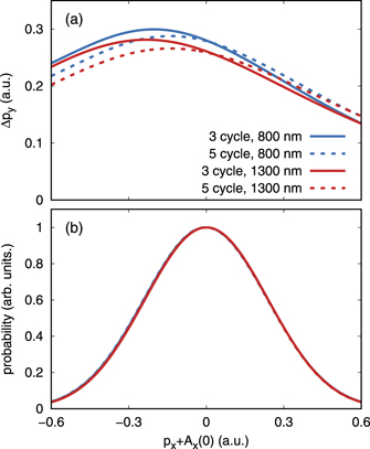
Figure 2. (a) Momentum-dependent attoclock shift as a function of px + Ax (0) and (b) slice through the probability distribution (at py = 0) for selected effective wavelengths and pulse durations. The other parameters are the same as in figure 1. These results are extracted from 2D TDSE simulations. The probability distributions in panel (b) are on top of each other and cannot be distinguished in the graph.
Download figure:
Standard image High-resolution imageIn addition to the global attoclock shift, we can analyse the shift along py for each momentum in the px –pz -plane individually. We refer to this quantity as the momentum-dependent attoclock shift. As an example, figure 1(b) shows the signal in the pz –py -plane (at constant px = −Ax (0)) with each column being normalized independently. We determine the most probable momentum Δpy using a Gaussian fit for each momentum pz . The result is show as black line in figure 1(b). At pz = 0, this shift is equivalent to the global attoclock shift Δpmax. However, for non-zero pz we find smaller shifts reaching values as small as ≈0.16 a.u. at pz = 0.6 a.u. corresponding to only ≈60% of the global attoclock shift.
The momentum-dependent attoclock shift as a function of px and pz is depicted in figure 1(c). Again, at each px , pz , the shift is obtained from a Gaussian fit to the py distribution. For the three-cycle laser pulse used here, the maximal attoclock shift of Δpy ≈ 0.285 a.u. is not found exactly at px + Ax (0) = 0 but at a slightly smaller value px + Ax (0) ≈ −0.2 a.u. The momentum-dependent attoclock shift decreases as a function of px and pz when going away from this point. We attribute the slight asymmetry of the momentum-dependent attoclock shift as a function of px + Ax (0) to a tiny rotation of the probability distribution (by only ≈2° in the polarization plane) that is mostly caused by the deviation from a purely linearly-polarized field near t = 0. Hence, the asymmetry diminishes for longer laser pulses that would be usually used in an experiment, see figure 2(a).
3.2. Classical adiabatic model
The observed momentum-dependent attoclock shifts can be explained by means of a classical adiabatic model consisting of two steps [20, 64, 65]: (i) laser-induced ionization and (ii) acceleration of the electron in the laser field as well as the ionic potential. The ionization step launches an electron at time t0 with an initial velocity v0. In the adiabatic limit γ → 0 the initial velocity v0 is perpendicular to the electric field E(t0) at the instant of tunneling, v0 ⋅ E(t0) = 0 [64, 66]. Since the electric field is approximately linearly polarized along y near t = 0, the vy -component vanishes for ionization times t0 around t = 0 and the setting is nearly isotropic in the v⊥–vz -plane which is perpendicular to the electric field E(t0). Hence, in this case we can write the initial velocity as v0 ≈ v⊥ ex + vz ez .
After ionization, the acceleration of the electron by the electric field and the Coulomb force of the parent ion can be described by Newton's equation. It maps the initial conditions (t0, v0) to the final momenta p(t0, v0). If we first consider the potential-free case, the motion in the laser field only results in p = −A(t0) + v0. For our particular bicircular field (4), we find that in the vicinity of t = 0 the release time t0 is mapped to the py -component of the final electron momentum and the initial velocity v0 ≈ v⊥ ex + vz ez is mapped to the px - and pz -components [29]. Hence, a change of the initial time t0 leaves the px - and pz -components approximately unchanged and a change in the initial velocity leaves the py -component approximately unchanged. Thus, our bicircular field offers a clean setup to study effects of an initial velocity v0.
The influence of the Coulomb force leads to an additional momentum change ΔpC that is essential to explain the attoclock shift, because it modifies the mapping to the asymptotic momentum of the electron,

We assume that the electron trajectory starts at an initial position  , i.e. at the exit of the tunnel, where
  with the electric field strength E(t0) = |E(t0)|. During its motion in our quasi-linear field the electron is driven away from the parent ion and does not come back close to it (in contrast to pure linearly polarized fields). Hence, we assume that, in our case, it is a good approximation to treat the Coulomb field as a perturbation and evaluate its contribution to the final momentum by integration of the Coulomb force along a trajectory rL(t) governed solely by the laser field [64]:

The Coulomb force decreases rapidly with increasing distance from the ion. Hence, in the adiabatic limit of vanishing Keldysh parameter γ → 0, the change in momentum is acquired in a time much shorter than an optical cycle of the driving light field. In the relevant time window around t0, the driving field can be assumed to be constant and the light-field-driven trajectory can be approximated as

At the peak of the electric field (corresponding to t = 0) the derivative of the electric field  vanishes and, hence, the leading-order correction to equation (8) also vanishes. Thus, for times near t = 0, the light-field-driven trajectory of equation (8) is a good approximation. Inserting equation (8) in equation (7), the momentum change due to the Coulomb force in a bare −Z/r potential is given by (to second order in the initial velocity v0)
The momentum correction of equation (9) can be viewed as an expansion of the exact result in terms of the potential strength, represented by the charge Z, and the Keldysh parameter γ. The second term of equation (9) leads to some focusing in the velocity coordinate v0 in the sense that the momentum distribution gets narrower in px - and pz -directions compared to the distribution of initial conditions. In contrast, the first term of equation (9) points in the direction of the electric field E(t0). In the quasi-linear field, electrons that are liberated at the peak of the electric field (corresponding to t0 = 0) are thus deflected in py -direction. Within this simple model the momentum-dependent attoclock shift introduced in section 3.1 is given by ΔpC,y of equation (9). Obviously, this shift strongly depends on the tunnel-exit position r0 of the electron and, hence, the attoclock can be used as a 'nano-ruler' to investigate the tunnel-exit position.
In previous classical models it has usually been assumed that the tunnel-barrier width r0 depends only on the time t0 via the electric field strength E(t0) (compare, e.g. the reviews [37, 38] on the attoclock). In the simplest approach it is assumed that the electron tunnels adiabatically in a 1D cut along the direction of the laser field [67]. This is referred to as field-direction model (FDM). After a separation of coordinates a one-dimensional potential barrier is formed by an atomic potential −Z/r and the electric field of the laser. The other directions lead only to an increased effective ionization potential  such that the tunnel-exit position is given by [20]

The barrier width as a function of the vz
-component of the initial velocity is shown in figure 3(a). Here, a non-zero initial velocity leads to an increased width of the tunnel barrier. If the influence of the central potential at the tunnel exit is neglected (Z = 0), the tunnel-exit position simplifies to the result for a triangular barrier (referred to as  model)

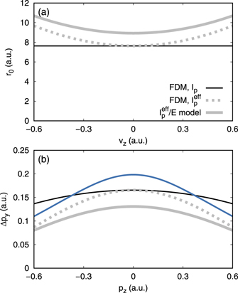
Figure 3. (a) Tunnel-barrier width as a function of the initial velocity vz
for ionization at t0 = 0. Shown are the  model of equation (11) (gray thick solid line) and the field-direction model (FDM) of equation (10) with velocity dependence (gray dotted line) or without velocity dependence, i.e. for v0 = 0 (black thin line). (b) Momentum-dependent attoclock shift as a function of pz
at fixed px
= −Ax
(0) ≈ 1.25 a.u. extracted from the solution of TDSE in 3D (blue solid line). In addition, the momentum shift ΔpC,y
of the model estimated by equation (9) is shown for the different choices of the tunnel exit from panel (a). The intensity is 4 × 10¹⁴ W cm−2 (Epeak = 0.101 a.u.) in both panels. The other parameters are the same as in figure 1.
model of equation (11) (gray thick solid line) and the field-direction model (FDM) of equation (10) with velocity dependence (gray dotted line) or without velocity dependence, i.e. for v0 = 0 (black thin line). (b) Momentum-dependent attoclock shift as a function of pz
at fixed px
= −Ax
(0) ≈ 1.25 a.u. extracted from the solution of TDSE in 3D (blue solid line). In addition, the momentum shift ΔpC,y
of the model estimated by equation (9) is shown for the different choices of the tunnel exit from panel (a). The intensity is 4 × 10¹⁴ W cm−2 (Epeak = 0.101 a.u.) in both panels. The other parameters are the same as in figure 1.
Download figure:
Standard image High-resolution imageThe attoclock shift as a function of the pz
-component of the momentum extracted from the numerical solution of the TDSE for an intensity of 4 × 10¹⁴ W cm−2 is shown in figure 3(b) together with the classical momentum shift ΔpC,y
that is estimated by equation (9) for different choices of the tunnel exit. In the classical model, larger tunnel-exit positions lead to a weaker influence of the Coulomb force on the outgoing electron and hence smaller attoclock shifts. Even though the classical momentum change ΔpC,y
for the FDM tunnel exit is overall slightly too small, the variation of the attoclock shift with momentum pz
is well reproduced. However, if the velocity dependence of the tunnel-exit position is artificially neglected by setting  , the variation of the attoclock shift as a function of pz
is drastically reduced. The difference between the shifts from the classical model including the velocity-dependent tunnel exit and the attoclock shifts from numerical TDSE calculations are at least partially caused by the adiabatic choice of the tunnel-exit position, the perturbative evaluation of the Coulomb correction and the approximated field-driven trajectory.
, the variation of the attoclock shift as a function of pz
is drastically reduced. The difference between the shifts from the classical model including the velocity-dependent tunnel exit and the attoclock shifts from numerical TDSE calculations are at least partially caused by the adiabatic choice of the tunnel-exit position, the perturbative evaluation of the Coulomb correction and the approximated field-driven trajectory.
A simple formula for the momentum change of the classical model as a function of the initial velocity can be obtained (to second order in v0) by using the  -tunnel-exit position of equation (11), leading to

The first term describes the global shift at v0 = 0 or equivalently at the final momenta px + Ax (0) = 0 and pz = 0, whereas the second term leads to the decrease of the shift as a function of px + Ax (0) and pz . Within this model, two thirds of the velocity-dependent term of equation (12) result from the dependence of the tunnel-barrier width r0 of equation (11) on the velocity and one third results from the linear velocity dependence of the trajectory (second term in equation (8)).
The classical model introduced in this section rests on two basic assumptions. First, both tunnel ionization and the subsequent Coulomb-induced momentum change of the outgoing electron are treated adiabatically, i.e. the electron velocity at the tunnel exit has no component along the ionizing field and the field is assumed to be constant during the short phase of Coulomb-induced acceleration. Second, the idea of the model is that the attoclock shifts in the final momentum distribution, which are obtained by peak search, correspond to ionization at the field maximum. We have attempted to refine this model by sampling the entire distribution of initial times and velocities in a classical trajectory Monte Carlo (CTMC) simulation as it has been successfully used to model the global attoclock shifts, e.g. in references [25, 39]. Here, the trajectories are weighted according to the Ammosov–Delone–Krainov rate [68] and for all trajectories, Newton's equation of motion are solved numerically with full inclusion of the external electric field and the Coulomb force. Afterwards, the attoclock shifts are extracted from the obtained final momentum distributions. In general, the CTMC method is expected to work well in the setup considered in the present work because interference between trajectories does not play a role. However, as far as the momentum-dependent attoclock shifts are concerned, we have found that the agreement with the TDSE results is not fully convincing as the momentum dependence is overestimated. We believe that this deficiency may be due to slight inconsistencies in the model such as the ad-hoc combination of initial distributions from quantum mechanical theories with the classical Newton's equation. Therefore, we do not show results from the CTMC method. In contrast, the simple classical model, consisting of the equations above, works surprisingly well as shown by our results below. Therefore, the discussion in the remainder of this paper focuses on the idea that the attoclock shifts correspond to ionization at the field maximum without taking the full distribution of initial conditions into account.
3.3. Scaling as a function of the light's intensity and wavelength
In the following, we employ the models of the attoclock shift for ionization occurring at the peak of the electric field, i.e. at t0 = 0 and E(t0) = Epeak. In this case, the simple formula of equation (12) suggests that the classical momentum change in the Coulomb field is a linear function of the electric field strength Epeak. For a systematic comparison between the models and the TDSE, we perform a series of calculations with varying peak field strength while keeping the vector potential Ax (0) fixed (by adjusting the wavelength). For sufficiently weak fields, we find indeed a linear field-strength dependence of the global attoclock shift Δpmax extracted from TDSE, see figure 4(a). The slightly increased slope observed in TDSE (compared to equation (12)) is partially caused by the approximated tunnel-exit position of equation (11) (compare the result using the FDM tunnel exit) and partially by non-adiabaticity: the Keldysh parameters γ are in the range between 0.28 and 0.57. For very strong fields, depletion effects play an important role so that the peak of the ionization rate shifts to earlier times and hence the attoclock shift from TDSE decreases [28, 31, 32].

Figure 4. (a) Global attoclock shift Δpmax as a function of the field strength. (b) Relative variation of the attoclock shift represented by the ratio  with Δpout being the attoclock shift at vout = 0.4 a.u. A sketch of the situation is shown in the inset of panel (a). (c) Tunnel-barrier width for vanishing initial velocity v0. (d) Velocity-dependent variation of the tunnel-barrier width represented by the ratio
  with rout being the tunnel-barrier width at vout = 0.4 a.u. The blue lines show the attoclock shift from 2D TDSE simulations for five-cycle laser pulses and the red lines are the results from classical backpropagation, see main text. The gray lines show the adiabatic estimate of equation (9) for the
  tunnel exit of equation (11) (gray solid lines) or the FDM of equation (10) (gray dashed lines). For each field strength, the vector potential Ax
(0) has been fixed to −3.32 a.u. (colored solid lines), −2.35 a.u. (colored dashed-dotted lines) and −1.66 a.u. (colored dotted lines) by scaling the wavelength in the numerical calculations.
tunnel exit of equation (11) (gray solid lines) or the FDM of equation (10) (gray dashed lines). For each field strength, the vector potential Ax
(0) has been fixed to −3.32 a.u. (colored solid lines), −2.35 a.u. (colored dashed-dotted lines) and −1.66 a.u. (colored dotted lines) by scaling the wavelength in the numerical calculations.
Download figure:
Standard image High-resolution imageTo quantify the relative variation of the attoclock shift as a function of the momentum by a single figure of merit, we define the relative difference M between the global attoclock shift and an outer attoclock shift

with Δpout being the attoclock shift at a given value of vout = px + Ax (0). In general, other measures could also be used, e.g. the curvature or the width of the momentum dependence, that would all allow for similar conclusions. For vout between 0.3 a.u. and 0.5 a.u., the same characteristic behavior of M is observed in the TDSE calculations. We present the results for vout = 0.4 a.u. as a function of the field strength Epeak in figure 4(b). The simple formula of equation (12) predicts that the relative difference M of the attoclock shift is independent of the field strength, see the gray horizontal line in figure 4(b). However, we find that the relative difference M from TDSE increases monotonically as a function of the electric field. This observation is in agreement with the classical momentum change of equation (9) when combined with the FDM tunnel exit of equation (10). Nevertheless, we note that for all considered field strengths, the numerical solutions of the TDSE suggest in the adiabatic limit a slightly smaller variation M compared to the classical model of equation (9).
3.4. Tunnel-exit positions from classical backpropagation
The main ingredient of the classical ad-hoc model presented in section 3.2 is the dependence of the tunnel-exit position r0 on the initial velocity v0 of the electron. The classical backpropagation introduced in section 2.2 offers the opportunity to extract such a correlation between the electron's initial conditions from ab initio calculations. Here, we again restrict ourselves to trajectories that depart from the tunnel barrier at the peak of the electric field strength, i.e. we analyse only those backpropagation trajectories for which the backpropagation stops at t0 = 0. Additionally, due to the nearly isotropic setting in the plane perpendicular to the direction of the instantaneous electric field it is sufficient to study the dependence along one coordinate axis of the initial velocity.
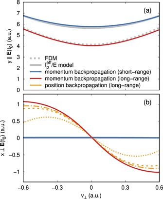
The y-component of the initial position parallel to the electric field E(t0) is shown in figure 5(a) as a function of initial velocity v⊥ in the polarization plane for an intensity of 1015 W cm−2. The backpropagation result for a long-range potential is in excellent agreement with the FDM of equation (10). As long as the ionization process is sufficiently adiabatic and over-the-barrier ionization is unimportant, this good agreement is also observed for a broad range of intensities, see figures 4(c) and (d). Increasing non-adiabaticity leads to slightly smaller exit positions of the electron compared to the static tunneling limit in agreement with references [31, 69].
Figure 5. (a) y-component of the tunnel-exit position as a function of the initial velocity v⊥ in the polarization plane for ionization at t0 = 0:  estimate of equation (11) (gray thick solid line), FDM of equation (10) (gray thick dotted line), backpropagation for a short-range potential (blue solid line) and for a long-range potential (red solid line). (b) x-component of the tunnel-exit position. In addition to the backpropagation described in section 2.2 (red solid line), results from the position-space based backpropagation method of [31, 32] are shown for different final times tf, namely tf = 0.5τ (dotted orange line), tf = 1.5τ (dashed orange line) and tf = 2.5τ (dashed-dotted orange line). Here, τ = 2π/ω is the length of an optical cycle of the laser field. All backpropagation results have been extracted from 2D TDSE calculations for the same laser parameters as in figure 1.
Download figure:
Standard image High-resolution image
The initial conditions from backpropagation can be used to start classical trajectories (propagating forward in time following Newton's equation). In analogy to the model in section 3.2, we determine numerically the momentum change ΔpC introduced in equation (6) due to the influence of the Coulomb force for these trajectories. The value of ΔpC,y for v0 = 0 as well as the corresponding relative variation are also shown in figures 4(a) and (b). Besides the plotted results for t0 = 0, we have confirmed that the values for the momentum change ΔpC,y depend only weakly on the exact initial time t0 in the vicinity of the peak of the electric field strength (not shown). For sufficiently low intensities (such that effects like depletion can be neglected) the global attoclock shifts extracted from TDSE follow indeed nearly the classical momentum change ΔpC,y from backpropagation. Here, the TDSE solution is consistent with the assumption of vanishing ionization times. However, for large intensities the classical momentum change ΔpC,y is larger than the global attoclock shift from TDSE. This indicates that the most probable ionization time is negative in this case which is in agreement with reference [29]. Nonetheless, the results from backpropagation reproduce the variation M of the attoclock shift very well, see figure 4(b). These theoretical findings support the interpretation that the momentum-dependent attoclock shifts are strongly affected by the velocity-dependent tunnel-exit positions.
Additionally, we have also studied the tunnel-exit positions for a 2D short-range potential

with the correct ionization potential of helium. The y-component of the initial position from backpropagation is in very good agreement with the simple  estimate of equation (11) and a quadratic dependence on v⊥ is clearly visible, see figure 5. This is expected as the strong-field approximation (SFA) (in saddle-point approximation) [66, 70, 71] typically describes the ionization dynamics for short-range potentials very well. Within this theoretical framework, the momentum-space based backpropagation can be carried out analytically (to exponential accuracy) resulting in the well-known exit position

where ts is the complex-valued saddle-point time. In the adiabatic limit this expression reduces to the estimate of equation (11) [33].
Both the FDM, equation (10), and the SFA, equation (15), imply that electrons tunneling at the peak field strength (t0 = 0) appear in the direction of the instantaneous field E(t0) (here the y-direction). For short-range potentials, this assumption is consistent with the backpropagation results as the obtained x-component of the tunnel-exit position (that is perpendicular to the electric field E(t0) at the instant of tunneling) vanishes, see figure 5(b). Surprisingly, for long-range potentials, the backpropagation results in non-zero x-components of the tunnel-exit position for v⊥ ≠ 0. The x-components take values as large as 1 a.u. for v⊥ = −0.6 a.u. This correlation of initial momentum and initial position is not limited to the initial velocities in the polarization plane but we have observed it in any direction that is perpendicular to the direction of the laser electric field at the instant of tunneling. Moreover, we also have found this correlation for other lights fields (e.g. circularly polarized light) which shows that this finding is not limited to our bicircular field. In additional calculations, we could show that the absolute value of these additional position offsets depends only weakly on the intensity of the field (not shown). Hence, we expect that for sufficiently weak laser fields this component is unimportant compared to the (large) tunnel-barrier width in field direction (y-component).
The backpropagation results presented above have been calculated using the method introduced in section 2.2 which is based on the momentum-representation of the wave function. Compared to the previous implementations [32, 33] based on the position representation, our implementation is beneficial for two reasons: (i) only a relatively small region of the position space needs to be represented explicitly. This is especially beneficial for long-wavelength driving fields and in 3D calculations. (ii) The result for the tunnel-exit position is in good approximation independent of the time tf when the forward quantum propagation is stopped. A comparison between the two backpropagation versions in figure 5(b) shows that the result using the position-space implementation [32, 33] depends on the final time tf. For long times tf → ∞ it converges slowly against the momentum-space result. In the opinion of the authors, the momentum-space implementation appears to be the correct result for the backpropagation scheme.
4. Conclusion
We have studied strong-field ionization of helium in an attoclock setup, i.e. by observing the peak of the PMD after applying a tailored bicircular light pulse. The employed bicircular field approximates linear polarization close to the time of peak field strength, while the shape of the vector potential enables its use as an attoclock [29]. The Coulomb force on the outgoing electron shifts the most probable electron momentum along the direction of the instantaneous electric field. Previously, this momentum shift was only analysed at the global maximum of the momentum distribution. However, our numerical solution of the TDSE shows that the attoclock shift depends on which slice of the momentum distribution is analysed, i.e. it depends on the momentum component perpendicular to the instantaneous ionizing electric field. Using a classical model for the adiabatic limit we have found that the momentum-dependent attoclock shift is closely related to the dependence of the tunnel-exit position on the electron velocity at the instant of tunneling. This finding is supported by results for the tunnel-exit positions obtained using the classical backpropagation method.
In the future, the quasi-linear attoclock could enable the investigation of orientation-dependent ionization dynamics in molecules [52] and it has the potential to allow for the retrieval of molecular tunnel-exit positions. Furthermore, the generalization of our findings to electric-field shapes that are not quasi-linear (e.g. close-to-circularly polarized fields [40]) will be interesting, because this involves the transfer of angular momentum in the tunneling process.
Acknowledgments
We thank Nicolas Eicke and Paul Ophardt for useful discussions. SB thanks the German Academic Exchange Service (DAAD) for financial support. We acknowledge funding of the DFG through Priority Programme SPP1840 QUTIF.
Data availability statement
The data that support the findings of this study are available upon reasonable request from the authors.
Footnotes
- 3