

Abstract
Topological many-body phases of matter exhibit remarkable electronic properties and ultracold atoms in optical lattices constitute promising candidates to study them in a well-controlled environment. In two-dimensional (2D) electron gases topological phases may emerge in the presence of strong magnetic fields. This situation is not directly applicable to cold atoms because they are charge neutral. Therefore, novel experimental techniques have been developed to engineer novel lattice systems, whose Hamiltonian is formally equivalent to the one of charged particles in magnetic fields. In this Tutorial, we introduce a paradigmatic topological lattice model, the Hofstadter model, and explain how it can be implemented with ultracold atoms using laser-assisted tunneling. The technique is based on imprinting phases on the tunneling matrix elements using additional laser beams. These phases are reminiscent of Aharonov–Bohm phases and can be interpreted as a magnetic flux piercing the lattice unit cell. We present experimental results on the cyclotron-like dynamics of neutral atoms in isolated four-site square plaquettes and discuss the first measurement of a 2D topological invariant, the Chern number, in artificially generated Hofstadter bands. The work presented in this Tutorial was one of the four shortlisted finalists of the 2016 DPG SAMOP dissertation prize.
Export citation and abstract BibTeX RIS
1. Introduction
With the discovery of the integer quantum Hall (QH) effect [1, 2] a new family of quantum states was found that did not fit into the usual classification of condensed matter systems [3–5]. Remarkably, a QH insulator is insulating in the bulk and displays current-carrying edge states [1, 2] at the boundaries. The quantization of the conductance is incredibly robust and independent of the microscopic details of the material [6, 7] due to the underlying topological properties of the system [8–10].
The concept of topology originally emerged from the study of geometric objects, whose surface topology can be used to classify them. Later these ideas have been applied to condensed matter systems. It was found that the intriguing electronic properties of QH insulators are intimately connected to the topological invariants, so-called Chern numbers, characterizing its energy bands [7]. Two condensed matter systems with a gapped energy spectrum are said to be topologically equivalent, if their spectrum can be continuously transformed into one another without closing the gaps.
It was known that topological quantum states may exist in two-dimensional (2D) systems with broken time-reversal (TR) symmetry. Since then many other topological materials have been found [3, 5, 11], for instance, TR symmetric topological insulators [12–16] in 2D [17–19] and even 3D systems [20, 21]. While all these materials can be understood in a single-particle framework, even more intriguing properties can occur in the presence of interactions. A prominent example are fractional quantum Hall insulators [22, 23], whose elementary excitations are predicted to exhibit fractional statistics that are neither fermionic nor bosonic.
To date, topological systems have been studied in a variety of different platforms ranging from photonics [24] to mechanical systems [25] and ultracold atoms in optical lattices [26, 27], see also the recent review [28] for additional references. Cold-atom settings are promising platforms for entering the regime of topological many-body physics [29, 30]. However, since atoms are charge neutral they are not subject to the Lorentz force, which conceptually constitutes the simplest way to break TR symmetry. Thus, novel experimental methods had to be developed to engineer effective Hamiltonians that are formally equivalent to those of charged particles in magnetic fields [26, 31–34]. Indeed experimentalists managed to realize two distinct topological lattice models, the Haldane [35] and the Hofstadter model [36–38] based on Floquet engineering [39] via off-resonant [40] or resonant shaking, also known as photon- or laser-assisted tunneling [41–43]. Complementary techniques have been further demonstrated based on the idea of synthetic dimensions [44, 45] by coupling different internal [46–49] or momentum states [50].
Here we present an introduction into the physics and topological properties of the Hofstadter model and explain how they can be studied with ultracold atoms using laser-assisted tunneling in optical lattices [51].
2. Hofstadter model
The Hofstadter model describes the motion of a particle with charge q in a periodic potential in the presence of a magnetic field B. In the continuum the presence of an external magnetic field results in an energy spectrum that consist of highly degenerate Landau levels. On the other hand electrons in a periodic potential experience a quantized energy spectrum, whose energy bands are known as Bloch bands. As a consequence, the interplay between the two characteristic lengthscales, the lattice constant a and the magnetic length  , where ℏ = h/(2π) is the reduced Planck's constant, leads to a complex fractal energy spectrum known as Hofstadter's butterfly [36–38]. The only relevant parameter α = ΦB/Φ0 in this problem is the dimensionless magnetic flux per unit cell
  , where Φ0 = h/q is the magnetic flux quantum. In order to reconcile the two lengthscales and observe the fractal spectrum, α needs to be on the order of one. In normal materials the lattice constants are small, on the order of a few angstroms, therefore unfeasible large magnetic fields are required to study the properties of the Hofstadter model. A possible solution is the design of artificial materials with larger lattice constants [52–58] as demonstrated with graphene placed on a substrate of hexagonal boron nitride [59–61].
2.1. Tight-binding description
The dynamics of charged particles in a periodic potential can be described using the tight-binding approximation. The description is based on the standard orbitals of the atoms, with the assumption that the overlap between wavefunctions of electrons on neighboring sites is small. This is a valid assumption for low temperatures, where all particles occupy the lowest energy level. The corresponding Hamiltonian takes the following form

where  and
and  are the creation and annihilation operators on site (m, n) respectively, m is the site index along x and n the one along y. Electrons in the lattice can tunnel between neighboring sites with strength J, which determines the kinetic energy of the system. These hopping matrix elements are modified according to the Peierls substitution [62], if an external magnetic field B = ∇ × A is applied, here A is the vector potential. As a result, tunneling is accompanied by phases
  , i = {x, y}, commonly known as Peierls phases (figure 1) and the tight-binding Hamiltonian is modified accordingly as

Figure 1. Square lattice with magnetic field. Illustration of a square lattice with complex hopping matrix elements  and lattice constant a. The magnetic flux
  piercing one unit cell of the lattice (gray shaded area) is determined by the Peierls phases
  , i = {x, y}, with m and n labeling the lattice sites along the x- and y-axis Reprinted by permission from Springer Nature: [51]. © Springer International Publishing Switzerland 2016.
Download figure:
Standard image High-resolution imageThe Peierls phases are a manifestation of the Aharonov–Bohm phase experienced by a charged particle moving in a magnetic field

where ΦB is the magnetic flux through the area enclosed by the contour  [63]. Equivalently one can define the magnetic flux per lattice unit cell in units of the magnetic flux quantum as


For simplicity we will refer to Φ as the flux per unit cell of the lattice or the flux per plaquette. The reason for this will become apparent later.
2.2. Magnetic translation operators (MTOs)
In the presence of the vector potential A the discrete translation symmetry of the underlying lattice is no longer determined by the lattice translation operators. Even if the magnetic field B is homogeneous and invariant under discrete lattice translations, the vector potential giving rise to the complex tunnel matrix elements in (2) is generally not invariant under this translation. This prevents a direct application of the well-known Bloch theorem. Instead the new symmetries of the system are described by so-called MTOs [64–66], which are a combination of lattice translation and gauge transformation and can be expressed in the following form:

In order to find a complete set of commuting operators we require ![$[{\hat{T}}_{i}^{M},\hat{H}]=0$](https://content.cld.iop.org/journals/0953-4075/51/19/193001/revision2/jpbaac120ieqn10.gif) and
and ![$[{\hat{T}}_{x}^{M},{\hat{T}}_{y}^{M}]=0$](https://content.cld.iop.org/journals/0953-4075/51/19/193001/revision2/jpbaac120ieqn11.gif) [51, 67]. Let us consider a translation around a super-cell with dimensions k × l. For a homogeneous flux distribution one can show that the operators fulfill the following relation:
[51, 67]. Let us consider a translation around a super-cell with dimensions k × l. For a homogeneous flux distribution one can show that the operators fulfill the following relation:

Hence, for rational values of α = p/q ( ) the commutator
 ![$[{({\hat{T}}_{x}^{M})}^{k},{({\hat{T}}_{y}^{M})}^{l}\phantom{\rule{}{2.0ex}}]$](https://content.cld.iop.org/journals/0953-4075/51/19/193001/revision2/jpbaac120ieqn13.gif) vanishes if
vanishes if

This relation can be fulfilled by various super-cells, however, the smallest one is uniquely defined by kl = q. This cell is called magnetic unit cell and its area is determined by  , which is q times the area of the normal unit cell of the underlying lattice. It contains q non-equivalent sites, which gives rise to the fractal energy spectrum as a function of the applied field. The operators
  ,
,  and
and  defined in equation (2) form a complete set of commuting operators and one can find simultaneous eigenstates Ψm,n by formulating a generalized Bloch theorem based on the magnetic translation symmetries:

where k = (kx, ky) is defined within the first magnetic Brillouin zone (FBZ): −π/(ka) ≤ kx < π/(ka), −π/(la) ≤ ky < π/(la).
It is interesting to mention here, that the area of the magnetic unit cell is uniquely defined by α, its dimensions, however, are not, as illustrated in figure 2 for α = 1/4. A detailed computation of the MTOs for α = 1/4 and staggered flux distributions can be found in [51].

Figure 2. Magnetic unit cells of a square lattice with flux α = 1/4. The area of the magnetic unit cell (blue shaded area) is AMU = 4a2 and it contains q = 4 non-equivalent sites (black circles). As a result there are three distinct possibilities for the dimensions of the magnetic unit cell as illustrated in (a)–(c). Reprinted by permission from Springer Nature: [51] © Springer International Publishing Switzerland 2016.
Download figure:
Standard image High-resolution image2.3. Harper–Hofstadter Hamiltonian
The Peierls phases in Hamiltonian (2) depend on the particular gauge chosen for the description. However, physical observables do not depend on the gauge and one can always choose to work with a certain gauge that simplifies the calculations. In this chapter we will use the Landau gauge ϕm,n = (−Φ n, 0), where Hamiltonian (2) transforms to

commonly known as Harper–Hofstadter Hamiltonian [36–38]. In this gauge only tunneling along the x-direction is accompanied by Peierls phases, while hopping in the perpendicular direction remains real. The energy spectrum of this Hamiltonian exhibits a fractal self-similar structure as a function of the flux α, which is known as Hofstadter's butterfly [38] and is shown in figure 3(a).

Figure 3. Magnetic field dependence of the Hofstadter energy spectrum. (a) Energy spectrum of the Harper–Hofstadter model as a function of the flux per unit cell α = Φ/(2π), known as the Hofstadter butterfly as explained in the main text. Example bandstructures are shown for α = 1/5 (b) and α = 1/6 (c). The integer values (green) on the right hand side of each spectrum indicate the Chern numbers of the corresponding well-separated energy bands. Reprinted by permission from Springer Nature: [51] © Springer International Publishing Switzerland 2016.
Download figure:
Standard image High-resolution imageFor rational values of the flux α = p/q the most convenient choice of the magnetic unit cell in the Landau gauge is the one oriented along the y-direction with dimensions (1 × q) · a2, because the MTOs take the simple form

They correspond to usual lattice translation operators, with the only difference that the translation along y is performed over an increased distance, namely q lattice sites. The magnetic unit cell contains a flux ΦMU = p × 2π. In accordance with the generalized Bloch theorem (9), one can make the following ansatz to solve the Schrödinger equation (SE)

The wavefunction Ψm,n is expanded in single-particle on-site wavefunctions ψi, j ≡ ψi, j ∣i, j〉, and kx, ky are defined in the range  and
and  . Indeed applying the MTOs defined in equation (11) one obtains

justifying the wavefunction ansatz equation (12). Inserting the latter into the SE associated with Hamiltonian (10),

one obtains an infinite number of relations

These equations can be recast into a q-dimensional eigenvalue problem

where H(k) is a q × q matrix of the following form:
with  . For
. For  there is no external magnetic field and one recovers a single energy band, with the tight-binding dispersion of a simple 2D square lattice

The corresponding bandwidth is Ebw = 2 × 4J. A rational flux per plaquette α = p/q leads to a splitting of this band into q subbands, Eμ(k), μ = {1, ..., q } resulting in a fractal spectrum (figure 3(a)). Figures 3(b), (c) show two exemplary bandstructures calculated for two different values of α. For irrational fluxes one obtains an infinite number of energy levels, which form a Cantor set [38].
2.4. Topological properties
The Hofstadter model is an important paradigmatic model for investigating the intriguing properties of topological phases of matter [3, 5]. It has motivated many theoretical and experimental studies also in artificial quantum systems [28]. It explicitly breaks TR symmetry and supports a series of QH and potentially fractional QH states [68–71]. QH insulators are characterized by a quantized Hall conductance [1, 2], which is directly related to the Chern number [7] of the occupied energy bands.
The Hall conductance σH is typically measured by sending a constant current through the material and observing the voltage difference that builds up across the sample perpendicular to the current. For low enough temperatures all energy levels below the Fermi energy EF are filled. Assuming that the Fermi energy lies between two bands the conductance is given by the sum of the contributions from all occupied bands Eμ < EF

where νμ is the Chern number of the μth band.
This is very interesting because QH systems are insulating in the bulk. Indeed the conductivity defined above results from the conducting edge modes, which are gapless and chiral. Each edge mode contributes one quantum of conductance e2/h, such that the magnitude of the Hall conductivity is only determined by the number of edge modes, which in turn is directly related to the Chern number of the bulk. Hence, the existence of edge states can be seen as a manifestation of the bulk topological order [7]. This correspondence explains the robustness of the Hall conductivity against small perturbations, since they do not change the topological properties of the energy bands determined by νμ
Here  are the periodic eigenfunctions, which are solutions of the eigenvalue equation (16), Ωμ(k) is the Berry curvature and the integral is performed over the first Brillouin zone (FBZ) [72]. The topological properties of the bulk are usually defined for an infinite system and its relation to the topological properties of the edge modes is commonly known as bulk-edge correspondence [8–10]. In section 7 we will discuss the first observation of a Chern number with charge-neutral particles [73].
Several properties of the Hofstadter model are worth mentioning here. Since the sub-bandstructure for a certain value of α emerges from a topologically trivial tight-binding band, the Chern number of the total band necessarily vanishes,  . One can further show that the particle-hole symmetry inherent to the model, results in a symmetric distribution of Chern numbers around zero energy (figures 3(b), (c)). Their values can be computed analytically based on a Diophantine equation [74, 75] or numerically for non-degenerate and degenerate bands following the work by Fukui et al [76].
3. Artificial magnetic fields
Since the physics of the Hofstadter model is difficult to access in real materials, in particular, if one aims at studying interacting topological phases, it is of large interest to consider engineered quantum systems [28], such as ultracold atoms. The latter can be efficiently trapped in periodic optical potentials [29, 77, 78], however, they are charge neutral which prevents a direct application of the Lorentz force. Hence, alternative experimental techniques had to be developed to mimic related effects, commonly termed artificial magnetic fields—a topic that is discussed in great detail in many review articles [26, 31–34]. We will only briefly mention a few techniques here and then focus on one specific method, known as laser-assisted tunneling.
Early experiments with harmonically trapped gases have exploited the equivalence between the Coriolis force in rotating traps and the Lorentz force [79–83] or engineered spatially-dependent optical couplings using Raman dressing [84, 85] as a successful way to simulate magnetic fields. Later Raman-assisted tunneling was proposed to engineer artificial magnetic fields in optical lattices [86–88], a technique well suited to enter the strong-field regime of one flux quantum per unit cell. Thus, giving access to the complex dynamics expected in the Harper–Hofstadter model [36–38]. The technique makes use of engineered couplings between the motional degrees of freedom in the lattice and the internal states of the atom. These pioneering ideas motivated several successive studies based on Floquet engineering [39]. The basic idea is to generate a time-dependent time-periodic system whose dynamics can be mapped to an effective time-independent Hamiltonian with the desired properties. Indeed experiments soon reported first realizations of complex tunneling matrix elements in 1D [89, 90] and 2D optical lattices [91, 92].
3.1. Effective Floquet Hamiltonian
Time-periodic Hamiltonians  can be treated using Floquet's theorem [93–95], which states that the evolution of the system after one period T = 2π/ω can be described by an effective time-independent Hamiltonian
  . The difficulty consists in finding an analytic expression for it and moreover in designing a time-dependent system whose effective Hamiltonian exhibits the desired properties. Within the scope of this tutorial we restrict ourselves to the high-frequency limit, where the frequency associated with T is large compared to the other energy scales, ℏω ≫ J, such that the Floquet Hamiltonian can be computed in a perturbative manner.
We start with a reminder on Floquet theory. In operator notation the time-dependent SE is

where  is the unitary time-evolution operator, that evolves a state
  at t = t0 to
  . In general it can be expressed as

where  is the time-ordering operator, i.e. a short notation of an infinite series of commutator relations. For periodic systems the evolution operator fulfills [96]

where  is the evolution operator over one period T. The long-time behavior of the system can be described stroboscopically with
  at times t = nT [93, 96–99] using an effective time-independent Floquet Hamiltonian

where  is a Hermitian matrix.
Note that this definition of  that describes the stroboscopic dynamics is not unique. There are several Hamiltonians that share the same spectral and topological properties, which only differ by a gauge transformation. The description is useful for a first analysis of the problem, however, for a complete discussion of experimental results the full-time dynamics has to be taken into account, since it may lead to additional oscillations in the observables [100–102]. This additional dynamics is sometimes called micro-motion. Its importance is nicely illustrated based on the example of Paul traps, where the motion of the particle in the time-dependent potential can be partitioned into a slow and a fast part, where the latter corresponds to the micro-motion, which oscillates at the frequency of the driving potential [103–105]. To treat the additional fast dynamics accurately one can use a more general form of Floquet's theorem, where the evolution operator is partitioned as [106]

Here ti,f denote the initial and final time of the evolution and we require that  is a time-periodic unitary operator. It contains information about the micro-motion and was given the intuitive name initial and final kick-operator in Ref. [100]. As mentioned above, the Hamiltonian
  and the operator
  can be calculated perturbatively in powers of 1/ω

The strategy is to compute  as a function of
  and to choose
  iteratively such that
  is time-independent. This assures that the effective Hamiltonian is time-independent in all orders n [100, 106].
It indeed works efficiently for Hamiltonians where the driving frequency is off-resonant compared to any intrinsic energy difference of the static Hamiltonian [40, 90, 91, 107–112]. This regime is fulfilled in lattice-shaking experiments. In particular lattice shaking was employed to simulate classical frustrated magnetism on a triangular lattice [91] based on the generation of staggered artificial magnetic fields. Later these ideas were extended to realize tunable Peierls phases in 1D lattices [90]. More recently off-resonant shaking was used to implement the topological Haldane model [40] and interaction-induced gauge fields [112]. For the experimental techniques discussed in this tutorial, however, the frequency ℏω is resonant with an energy scale in the static Hamiltonian [41–43, 73, 92, 113–116]. Thus, it diverges in the limit  , which, however, is the basic requirement for our perturbative expansion in equation (26). In the following two subsections, we will introduce two complementary methods to treat this problem: the first one is based on a formalism introduced by Rahav et al (section 3.1.1) and the second one on the Magnus expansion (section 3.1.2).
3.1.1. Perturbative analysis: resonant driving
We start by writing the static Hamiltonian as
where  is a projection operator. The integer β labels orthogonal sectors,
  and
and  [102]. This notation is useful for the treatment of distinct static lattice potentials and the number of sectors β will depend on it. For instance, figure 4(a) illustrates a staggered superlattice potential, where the potential energy of every other site is increased by ℏω and hence, β = {0, 1}. We will provide more specific examples in section 3.3. In general, terms of the form
  describe additional potential energy offsets or equivalent diagonal terms, while
  (β
(β  γ) couple different sectors. We assume that all terms that diverge with ω are contained in the diagonal components of the static Hamiltonian and all remaining ones do not diverge. Similar to the static terms we write the time-periodic part

Figure 4. Schematic drawings of periodically modulated 1D lattices. In both situations there is a potential energy offset between neighboring sites Δ ≫ Jx, which inhibits tunneling. Periodic modulation at frequency ℏω = Δ can restore resonant tunneling in both lattice potentials. (a) Superlattice potential with two non-equivalent sites (β = {0, 1}) and energy offsets Δm = (−1)m Δ/2. (b) Wannier–Stark ladder with linearly increasing on-site energy Δm = m Δ (β = {0, 1, 2, 3, ...}). The colored energy levels refer to different sectors β. Adapted figure with permission from [102], Copyright (2015) by the American Physical Society.
Download figure:
Standard image High-resolution imageTo treat the diverging terms we apply a time-dependent unitary transformation to the total Hamiltonian  [102]:
This results in the transformed Hamiltonian


which is indeed time-periodic and does not contain any divergent terms that scale with ω. Moreover we can directly apply the formalism [100] introduced above. In accordance with equation (25) the full-time evolution operator of the transformed systems is

where from now on we refer to  as the micro-motion operator, which is a combination of the kick-operator defined above and the divergent terms of the static Hamiltonian. In the transformed system the Floquet Hamiltonian
  and the kick-operator
  can be expanded in orders of 1/ω and one obtains [100]


where terms  have been neglected for simplicity. This is a powerful approach for computing the full-time evolution of periodic Hamiltonians.
3.1.2. Magnus expansion approach
Alternatively the effective Hamiltonian can be calculated based on the Magnus expansion [117–119], which is particularly useful for describing the stroboscopic long-time evolution at integer multiples of the modulation period T, t = nT with  . An instructive comparison of the two methods for a simple double-well potential can be found in [51]. Similar to the discussion above, the Magnus expansion is a perturbative treatment, that works well in the high-frequency limit. The Floquet Hamiltonian is written as an infinite sum
  , where the lowest order is given by

and higher orders of the expansion scale as (1/ω)n. For  the time-independent Floquet Hamiltonian is well approximated by the lowest order
  . In this description it is easy to see that there is a family of Floquet Hamiltonians with similar properties, which can be obtained by changing the time interval chosen for the integration, e.g. t ∈ [t0, t0 + T]. All these results are related by gauge transformations [119] and share the same spectral and topological properties.
For Hamiltonians of the form (27), (28) we again have to treat the diverging terms separately. We perform a slightly modified unitary transformation that includes explicitly the time-dependent term  [119, 120] using
The transformed Hamiltonian is denoted as  , which is again time-periodic and according to equation (35) the Floquet Hamiltonian can be approximated by

3.2. Two-level system
Let us start by illustrating the basic operating principle of laser-assisted tunneling using a two-level system with states  and
and  . The two levels are separated by a large energy Δ and the system can be described by the static Hamiltonian

where J denotes the coupling strength between the levels, which is small compared to Δ. Due to the non-zero coupling J there is finite mixing of the two levels and the eigenenergies are separated by

which sets the exact value for the resonance condition ℏω = Egap, where the two eigenstates are resonantly coupled. In actual experiments this is usually automatically ensured by the calibration measurements. If this is not the case, the dynamics can be largely modified if the system is modulated at ℏω = Δ [51, 101].
In the limit of a large energy offset Δ ≫ J the equation simplifies and the resonance condition is approximately given by Egap ≃ Δ = ℏω. The dynamics of the resonantly-driven system is then described by the time-periodic Hamiltonian

with  the projectors on the two sectors β = {0, 1} and V0 the modulation amplitude. Following the theoretical description presented in section 3.1.2 we transform the system into the rotating frame [119, 120] according to equation (36) with

This transformation effectively introduces the time-dependence into the coupling term and we obtain
The transformed Hamiltonian  is time-periodic without any static components. To lowest order (equation (37)) the Floquet Hamiltonian can be written as

where  is the first-order Bessel function of the first kind. The coupling between the two levels
  and
and  is resonantly restored, renormalized and accompanied by an additional term
  . It can be interpreted as a Peierls phase and is well suited to realize artificial magnetic fields (section 3.4). One can further show that for systems described by Hamiltonians of the form (38), the micro-motion operator in the lab-frame is to lowest order determined by the operator
  in equation (41). Note, however, that this is not true in general.
The resonantly coupled two-level example can be straightforwardly extended to a more general situation, where coupling is restored for energy offsets that are equal to an integer multiple of the modulation frequency Δ = νℏω, with  [121, 122]. These situations are also termed multi-photon processes, since multiple quanta of the driving field are required to bridge the energy gap Δ. The associated Floquet Hamiltonian in the rotating frame is

where  denotes the ν-order Bessel function of the first kind. While for zero-order processes (ν = 0) the couplings remain real and are renormalized by
 ![${{ \mathcal J }}_{0}({V}_{0}/[{\rm{\hslash }}\omega ])$](https://content.cld.iop.org/journals/0953-4075/51/19/193001/revision2/jpbaac120ieqn71.gif) [107], first-order processes (ν = 1) lead to complex tunneling matrix elements and are typically termed photon- or laser-assisted tunneling [113]. Note that the phase factors depend on the resonance conditions, as summarized in the table below.
[107], first-order processes (ν = 1) lead to complex tunneling matrix elements and are typically termed photon- or laser-assisted tunneling [113]. Note that the phase factors depend on the resonance conditions, as summarized in the table below.
| Resonance cond. | Eff. coupling strength | Phase factor |
|---|---|---|
| ℏω = Δ |
![$J{{ \mathcal J }}_{1}({V}_{0}/[{\rm{\hslash }}\omega ])$](https://content.cld.iop.org/journals/0953-4075/51/19/193001/revision2/jpbaac120ieqn72.gif)
|
φ |
| ℏω = −Δ |
![$J{{ \mathcal J }}_{1}({V}_{0}/[{\rm{\hslash }}\omega ])\,$](https://content.cld.iop.org/journals/0953-4075/51/19/193001/revision2/jpbaac120ieqn73.gif)
|
−φ + π |
3.3. Periodically driven 1D lattices
In the previous section we have introduced the problem of a resonantly coupled two-level system from a stroboscopic point of view based on the effective Hamiltonian  . In an actual experiment the micro-motion
  may, however, have a large impact on experimental observables. Here, we will study its properties by means of a few specific examples. Common laser-assisted tunneling schemes rely on potential energy offsets Δm along one of the two lattice axes to inhibit tunneling, which can then be restored resonantly with the modulation.
We start our discussion with resonantly-driven 1D lattices and then extend it to the 2D situation in the next section. In particular we present two examples illustrated in figure 4, which are described by the tight-binding Hamiltonian


where φm is the site-dependent phase of the time-dependent potential and Jx is the tunnel coupling along x. In the following we consider only potentials with Δm+1 − Δm = ±Δ = ±ℏω but the model can be straightforwardly extended to more general energy landscapes [102]. Hamiltonian (46) is indeed time-periodic  and of the form defined in equations (27), (28). The static divergent term can be written as

where  is the number operator for the sector β and
  . Each sector is composed of several sites m, which are defined by the specific form of the on-site potential Δm. The staggered superlattice potential (figure 4(a)) separates into two different sectors β = {0, 1}, where every other lattice site belongs to the same sector. The Wannier–Stark ladder (figure 4(b)) instead consists of an infinite number of sectors, each of them containing only a single site. Independent of β the number operator
  can be expanded in terms of projectors

Using this equation and equation (47) one obtains

Following the theoretical description presented in section 3.1 we find the micro-motion operator
where we have applied the unitary transformation defined in equation (36) with the approximation ![$\exp [{\rm{i}}{ \mathcal M }(t)]\simeq \hat{R}(t)$](https://content.cld.iop.org/journals/0953-4075/51/19/193001/revision2/jpbaac120ieqn80.gif) . The transformed Hamiltonian reads
. The transformed Hamiltonian reads

with ηm(t) = χm+1(t) − χm(t) given by

Here ![${\eta }_{0}=2{V}_{0}/({\rm{\hslash }}\omega )\sin [\delta \varphi /2]$](https://content.cld.iop.org/journals/0953-4075/51/19/193001/revision2/jpbaac120ieqn81.gif) is the differential modulation amplitude and δφ = φm+1 − φm.
is the differential modulation amplitude and δφ = φm+1 − φm.
Looking at equation (50) we find that  is proportional to the number operator
  . As a consequence it commutes with any terms of the effective Hamiltonian proportional to
  and hence the density distribution of the eigenstates remains unaffected during one cycle in contrast to the quasi-momentum distribution [116], which is a typical observable probed with Bose–Einstein condensates (BEC) after standard time-of-flight (TOF) imaging [29]. The micro-motion operator consists of two distinct parts, one associated with the time-dependent potential proportional to γ = V0/(ℏω) and a second one introduced by the static potential Δm. The first one gives rise to additional momentum components at positions related to the phase distribution φm. The amplitudes of these components oscillate periodically in time but their position remains unchanged. Their contribution to the signal vanishes in the high-frequency limit
  . The second term depends highly on the shape of the static potential. For the staggered superlattice
  (figure 4(a)) additional momentum components appear at ±π/a, which oscillate in amplitude with period T = h/Δ but no additional components are populated during one cycle. This dynamics persists even in the limit
  . For the Wannier–Stark ladder Δm = mΔ (figure 4(b)) the corresponding term is associated with a constant drift in momentum space, δk(t) = ωt/a with constant amplitudes [116]. Consequently, all laser-assisted tunneling techniques based on Wanner-Stark ladders exhibit such a drift, also known as Bloch oscillations [123].
3.4. Extension to 2D: artificial gauge fields
The complex couplings in 1D are mere gauge transformations and the system remains trivial. Extending those settings with a second perpendicular lattice potential enables the engineering of more interesting situations. We consider the following time-dependent Hamiltonian
where Jy is the tunnel coupling along the perpendicular axis and tunneling is inhibited along the x-axis for Δ ≫ Jx and V0 = 0. Note, that the modulation potential involves a phase distribution φm,n that varies along both axes. Analog to the 1D case we find the micro-motion operator
and the transformed Hamiltonian
Indeed the periodic modulation generally affects tunneling along both directions. The functions  and
and  are determined by


For  tunneling can be resonantly restored with ℏω = Δ (laser-assisted tunneling) and one obtains the effective time-independent Hamiltonian
where the Peierls phases ϕm,n ∝ (φm+1,n + φm,n)/2 depend on the distribution φm,n and on the on-site potential Δm (section 3.2). Along y tunneling is renormalized and in the high-frequency limit ( ) one finds
which means it decreases with increasing γ. How strongly it decreases depends on the phase difference of the modulation between neighboring sites δφy = φm,n+1 − φm,n (figure 5(a)). For in-phase modulation the relative phase difference vanishes (δφy = 0) and the bare tunneling remains unchanged.

Figure 5. Effective tunnel coupling for zero- and first-order assisted processes. (a) Tunneling in the y-direction is renormalized proportional to  , where the argument of the Bessel function depends on the driving amplitude in units of the driving frequency γ = V0/(ℏω) and the relative phase difference δφy = φm,n+1 − φm,n as defined in equation (58). (b) Along x tunneling is resonantly restored according to
  . Its amplitude depends on the relative strength of the driving γ and the phase difference between neighboring sites δφx = φm+1,n − φm,n. The side panels in each subfigure display the effective couplings for parameters marked by the red dashed lines. Reprinted by permission from Springer Nature: [51] © Springer International Publishing Switzerland 2016.
Download figure:
Standard image High-resolution imageIn the perpendicular direction (x-axis) tunneling is resonantly restored, resulting in an effective tunnel coupling  . Its amplitude again depends on the relative phase difference δφx = φm+1,n − φm,n (figure 5(b)) and it is proportional to the driving amplitude γ. In the limit of large ω (
 ) it can be approximated by

Again for in-phase modulation (δφx = 0) only a global energy shift is modulated in time, which cannot be used to restore tunneling. However, this is precisely how one can engineer more complex modulation geometries, which enable a local control of laser-assisted tunneling in the lattice; further details are discussed in [51].
The Peierls phases ϕm,n in Hamiltonian (59) appear only in the coupling terms with restored tunneling (x-axis). Note, that they give rise to a flux Φm,n = ϕm,n − ϕm,n+1 per plaquette (defined along + ), whose value depends on the phase evolution in the perpendicular direction δφy, while the amplitude of the coupling K depends on δφx. The laser-assisted-tunneling scheme presented here naturally generates artificial fluxes on the order of
  and therefore constitutes a good candidate to enter the strong-field regime required to study the Hofstadter model. Related techniques have been further identified, e.g. for ions or superconducting circuits [28].
4. Optical lattices and superlattices
Within the scope of this tutorial several experimental configurations for the generation and study of artificial magnetic fields are going to be discussed. The optical potentials can be categorized in two different groups: the static lattice potentials and the far-detuned running-wave beams employed to induce laser-assisted tunneling. In figure 6(a) an overview of the various static lattice potentials is shown, which are used to create lattice potentials of different dimensionality and with different unit cells. All lattice laser beams are focused on the atoms and retro-reflected in order to create a standing wave potential of the form  , where Vx is the potential depth and k = 2π/λ the wavevector of the light. Depending on the detuning of the laser beam relative to the internal atomic transition the atoms are located either in the intensity minima (blue-detuned) or maxima (red-detuned) of the standing wave potential [124]. The lattice constant of the optical crystal is determined by a = λ/2. In the horizontal plane so-called superlattice potentials enable the generation of optical lattices with larger unit cells [125, 126]. A single superlattice along one axis, e.g. the x-direction, is created by superimposing two standing waves (figure 6(b)) with different wavelengths, here λl = 2λs. The combined potential is given by

where the index l(s) denotes the parameters of the long (short)-wavelength lattice and θ is the relative phase between the two. Depending on θ different potential landscapes can be engineered as displayed in figure 6(c). For moderately deep lattice potentials and low temperatures the system is described by the Bose–Hubbard Hamiltonian [127]. Since most of the experiments are performed in the weakly-interacting limit, where the interactions between the atoms can be neglected, the dynamics can be described the following Hamiltonian

where  denotes nearest-neighbor pairs and the tunneling matrix element Jm,n generally depends on the position in the lattice as induced by the superlattice potentials (figure 6(c)).

Figure 6. Schematic of the general lattice and superlattice setup. (a) Overview of the static lattice potentials created with wavelengths λz (red-detuned), λs (blue-detuned) and λl = 2λs (red-detuned). Superlattice potentials can be generated along the x- and y-direction by superimposing two standing waves with λs and λl. Reprinted by permission from Springer Nature: [51] © Springer International Publishing Switzerland 2016. (b) The shape of the superlattice potential depends on the relative phase θ between the two standing waves. (c) Examples for superlattice potentials with θ = 0 (symmetric double well) and θ = π/2 (staggered superlattice potential) as defined in equation (62), with tunnel coupling Jx and energy offset Δ between neighboring sites. Odd lattice sites (black circles) denote sites of low on-site energy and even lattice sites (white circles) the ones of high energy. Adapted by permission from Springer Nature: [114] © Springer-Verlag Berlin Heidelberg 2013.
Download figure:
Standard image High-resolution image5. Staggered magnetic fields
First experimental realizations of artificial magnetic fields in optical lattices have been obtained with staggered-magnetic-flux distributions [41, 91, 92, 109], whose bandstructure is topologically trivial but gives rise to interesting properties [109] in particular if interactions are introduced into the system [128]. We are going to discuss an example based on a staggered optical superlattice potential (figure 6(c)) following [92] which was inspired by early theoretical works [86, 87, 129]. The only difference compared to these ideas is that here the internal structure of the atom does not play any role [130–133]. This has the advantage that it is applicable to any species and does not suffer from heating due to spontaneous scattering of photons as expected for schemes based on near-resonant light. All results presented in the scope of this tutorial were obtained with bosonic atoms, but the experimental techniques can be applied equally well to fermions. Using the laser-assisted-tunneling scheme introduced in section 3.4 together with a staggered optical potential results in a flux distribution that alternates in sign along the axis with restored tunneling, while it is uniform along the other with a zero mean value.
5.1. Experimental setup
The 2D lattice potential consists of a simple lattice along y generated at wavelength λs and a staggered superlattice potential along x with a staggered potential energy offset ±Δ/2 as illustrated in (figures 6(b), (c)). In the following we use the convention that high-energy sites are even lattice sites. For large energy offsets Δ ≫ Jx the dynamics along x is frozen, while atoms tunnel freely along y. The time-dependence is introduced with an additional pair of far-detuned running-wave beams with wavevectors  and frequencies ω1,2. As shown in figure 7(a), each of them is aligned along one of the main lattice axes. Tunneling along x is resonantly induced for ω = ω1 − ω2 = ±Δ/ℏ. The two beams interfere and create a local time-dependent potential of the form

with δk = k1 − k2 and ϕ0 = ϕ1 − ϕ2. Strictly speaking there is an additional static term, which we have neglected because it only leads to a global energy shift. The relevant terms in VK(r, t) are the site-dependent phases given by δk · R = kRa (m − n), where  defines the position in the lattice and
  are the unit vectors. For the implementation reported in [92] kR = π/(2a) and the phases are given by

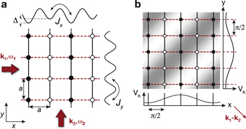
Figure 7. Laser-assisted-tunneling setup for the generation of staggered artificial magnetic fields. (a) 2D lattice with constant a = λs/2 and tunnel coupling Jy along y. The lattice is modulated by two running-wave beams (red arrows) with frequencies ωi, i ∈ {1, 2} and wavevectors  . Resonant tunneling is induced for
  . Reprinted by permission from Springer Nature: [51] © Springer International Publishing Switzerland 2016. (b) Local optical potential Vk at a fixed time t, which is created by the interfering beams and
  . The phase fronts (line of same color) determine the phase distribution φm,n of the time-dependent potential in equation (64). Adapted by permission from Springer Nature: [114] © Springer-Verlag Berlin Heidelberg 2013.
Download figure:
Standard image High-resolution imageAlong both lattice axes the phase advances by δφx = −δφy = π/2 as shown in figure 7(b). This value can be easily modified by changing the geometry of the running waves or a different ratio kR/a, such that any value of the flux becomes accessible. In equation (64) there appears an additional phase offset ϕ0, which is the relative phase between the two beams. In the experiment it is not actively stabilized and varies randomly for each realization but it has not influence on the distribution of artificial fluxes.
The dynamics of the system is described by a time-periodic Hamiltonian  of the form (53) with Δm = (−1)m Δ/2 and
  being the site-dependent phases generated by the running-wave beams (figures 7(a), (b)). As discussed in section 3.1 in the high-frequency limit ℏω ≫ Jx, Jy the stroboscopic evolution of the system can be described by an effective time-independent Hamiltonian of the form
with  and
and  . Due to the staggered energy offset the phase distribution ϕm,n is non-uniform (section 3.2) and varies according to
The distribution depends on the chosen laser-assisted-tunneling geometry and for the setting depicted in figure 7(a) the on-site phases are  and one finds the corresponding Peierls phases
For simplicity we set ϕ0 = −3π/4 and rewrite the expression for the phases as

This distribution gives rise to a staggered flux distribution  with zero mean. It is uniform along y and staggered along x [92, 114].
The micro-motion operator required to understand the full-time evolution of the system is defined in equation (54). It leads to a very similar behavior as in the case of a periodically modulated 1D staggered superlattice potential (section 3.3). The part related to the staggered on-site potential Δm is trivial because it only leads to oscillations in the amplitudes of the individual momentum components. The modulation-induced term, however, gives rise to additional momentum components shifted by multiples of δk = (π/(2a), π/(2a)) and influences the measured momentum distributions presented in the following section.
5.2. Ground-state properties
In order to study the ground-state properties of the effective Hamiltonian defined in equation (66) we prepared a BEC in the lowest band of a 2D optical lattice with Jx/h = Jy/h = 31(2) Hz, which results in a 2D array of coupled 1D Bose gases, as reported in [92]. Then we ramped up the staggered potential energy offset Δ/h = 4.4(1) kHz within 0.7 ms. Subsequently, the lattice along x was decreased and the modulation was turned on to induce resonant tunneling along that axis with an effective coupling strength K/h = 30(2) Hz.
This is a highly non-adiabatic experimental protocol which was optimized experimentally. We found that after about 10 ms the phase coherence was restored, most likely because of entropy redistribution along the longitudinal modes. The quasi-momentum distribution was then observed after suddenly releasing the atoms and 20 ms TOF (figure 8(a)).

Figure 8. Momentum distribution of the ground-state wavefunction. (a) The momentum distribution was probed with a BEC in the ground state of a lattice with staggered flux Φ = (−1)m+1 π/2 and J/K = 1.0(1) after 20 ms TOF (left panel), where ks = 2π/λs. The right panel displays the expected distribution calculated by exact diagonalization of a 31 × 31 lattice with harmonic confinement ωx/(2π) = ωy/(2π) = 20 Hz. The first magnetic BZ is indicated by the red rectangle and the zero momentum is marked by a red cross. The magnetic BZ contains two momentum components shifted by δk (red arrow). Each image was normalized to its maximum intensity. (b) Projection of ground-state momenta along y for different J/K. There is a bifurcation point at  as indicated by the solid lines obtained based on the eigenvalue equation (71). For smaller values (
 ) there is a single momentum component ko (black) with koy = ks/4, while for larger values there appear two components denoted as
  (dark blue) and
  (light blue). These components approach
  and
and  for J ≫ K. The insets display the calculated momentum distributions in the FBZ and the red cross marks the position of zero momentum. The horizontal error bars indicate calibration uncertainties of J/K and the vertical ones are fitting errors in determining the positions of the momentum components. Reprinted figure with permission from [92], Copyright (2011) by the American Physical Society.
Download figure:
Standard image High-resolution imagePerforming the same measurements with a simple cubic lattice and Φ = 0 would result in a single momentum component in the FBZ at kx = ky = 0 and additional ones at multiples of the reciprocal lattice vectors (2ks, 0) and (0, 2ks), where ks = π/a. For the staggered flux lattice instead four momentum components per cubic lattice BZ were found. The observed distribution can be understood by solving the SE using the following ansatz for the wavefunction
Note that, due to the magnetic translation symmetries, the magnetic unit cell is two times larger than the usual lattice unit cell with dimensions 2a × a. Using the above ansatz we can reduce the problem to a 2D eigenvalue equation  with
with
where kx, ky are defined within the FBZ, −ks/2 ≤ kx < ks/2 and −ks ≤ ky < ks, and ψe,o are the amplitudes on even and odd lattice sites respectively.
For equal couplings J/K = 1 a single energy minimum in the dispersion relation is found at ke = (−ks/4, −ks/4). The corresponding ground-state wavefunction has equal amplitudes on all sites,  . According to the intrinsic structure of the eigenstates defined in equation (70) two momentum components are expected: one at ke and an additional one at ko = ke + δk, with δk = (ks/2, ks/2). The second one is due to the additional phase factor of the wavefunction in equation (71) for odd lattice sites. The measured TOF images further show momentum components separated by the reciprocal magnetic lattice vectors (ks, 0) and (0, 2ks) as displayed in figure 8(a). The observed momenta are in agreement with theory.
The remaining question concerns the effect of the micro-motion operator on the measured distributions, since so far we have only discussed the results in comparison with the Floquet Hamiltonian (66) in the rotating frame. The term that may lead to additional momentum components (section 3.3) is proportional to V0/(ℏω), which for our experimental parameters is not negligible V0/(ℏω) ≃ 0.48. Indeed as can be seen in figure 8(a) there are two weak additional quasi-momenta in the FBZ located at (−ks/4, 3ks/4) and (ks/4, − 3ks/4) in agreement the micro-motion operator defined in equation (54). Looking at the full-time dynamics one finds that there are small oscillations in the amplitudes of the individual quasi-momenta but their position remains constant. Note that it is important to express all the operators using the gauge realized in the experiment because the TOF images depend on that [128, 134, 135]. For a different choice of the vector potential the momentum components would appear at different locations in the FBZ [51]. Intuitively this can be understood as follows: in TOF measurements all potentials are rapidly switched off and the system evolves according to the free-particle Hamiltonian. After long enough expansion times the images provide the Fourier transform of the condensate wavefunction. Phases that are imprinted on the condensate wavefunction, which is done in order to realize a particular vector potential, will directly show up as Fourier components in the TOF images, for instance, a constant phase difference between neighboring sites translates into a momentum shift of the distribution measured after TOF and hence, the particular gauge realized in the experiment will be visible in the TOF distributions.
Varying the coupling ratio J/K we find that there is a single minimum in the dispersion up to a critical value  , above which the system exhibits a two-fold degenerate ground state (figure 8(b)). In future experiments it would be interesting to study the ground state of weakly-interacting bosonic atoms in this lattice and try to detect the incommensurate charge density wave that is expected to form [128].
5.3. Local observation of the artificial magnetic flux
Superlattices enable powerful local measurements even without single-site resolution [136–141]. In a 2D superlattice (figure 6) tunneling can be inhibited on every other bond along both lattice axes (figure 9(a)). This restricts the dynamics to a minimal lattice that consists of only four sites  . Using an additional vertical lattice at λz a 3D array of isolated four-site square plaquettes is realized. By preparing a single atom inside one such plaquette potential one can study the influence of the artificial flux on its dynamics and extract the amplitude of the artificial field.

Figure 9. Cyclotron-like dynamics of single atoms. (a) Illustration of the experimental setup. A 2D superlattice potential restricts the dynamics to four-sites square plaquettes. An energy offset Δ is used to inhibit tunneling along x, which is restored resonantly using a pair of running-wave beams (figure 7) resulting in a flux Φ in each plaquette. The effective coupling strength is denoted as K and tunneling along y occurs with strength J. The dynamics is described by a 4 × 4 matrix defined in equation (72). The four individual sites are labeled as  . The initial state
  is indicated with the gray area. (b) Cyclotron orbit obtained from the mean atom positions
  and
and  . The inset shows the theoretical prediction obtained by solving the time-dependent SE numerically for Φ = 0.8 × π/2 and a 1/e-damping time of 13 ms. The latter was determined from damped-sine fits to
  and
and  . The damping is due to inhomogeneities caused by the harmonic trap, which leads to a dephasing of the oscillations between individual plaquettes. (c) Calculated full-time dynamics for the parameters used in the experiment (dashed line), V0/Δ = 0.39, K/h = 0.28 kHz and J/h = 0.47 kHz, in comparison with the ideal evolution expected from the effective Hamiltonian (72) (blue solid line). The dots highlight the stroboscopic dynamics obtained from the full-time evolution. (b) Reprinted figure with permission from [92], Copyright (2011) by the American Physical Society. (a), (c) Reprinted by permission from Springer Nature: [51] © Springer International Publishing Switzerland 2016.
Download figure:
Standard image High-resolution imageThe measurements are performed in a plaquette potential which has an energy offset Δ along x and no offset along y, such that tunneling is inhibited along the x-axis by Δ. It is then restored resonantly with the running-wave setup described in section 5.1. The sign of the flux in each plaquette depends on the sign of the energy offset Δ and since only every other plaquette contributes to the measured signal each of them exhibits the same flux because each of them has a potential energy difference of the same sign.
The experimental sequence started by preparing a single atom in the ground state of the tilted plaquette  with Jx/h = 1.2(1) kHz, Jy/h = 0.5(2) kHz and Δ/h = 4.9(1) kHz, as reported in [92]. To initiate the dynamics we suddenly turned on the modulation with V0/(ℏω) ≃ 0.34, K/h = 0.28(1) kHz and J ≃ Jy. The following evolution is governed by the effective Hamiltonian, which can be expressed as a 4 × 4 matrix
  . We choose the basis
  and obtain

with Φ = π/2.
Experimentally we determine the real-space dynamics by measuring the site occupations in the plaquette  as a function of time using a site-resolved band-mapping technique [125, 126]. From this we compute the mean position of the atom in the plaquette


where N is the total atom number (figure 9(b)). There is an important difference between these measurements compared to conventional high-resolution detection techniques [136–141]. The measurements are performed simultaneously in a 3D array of plaquettes and one obtains averaged observables without true local information. The evolution starts at  and
and  with all atoms delocalized over the left bond. Shortly after tunneling is restored the atoms tunnel to the right (B- and C-sites) and without flux one would expect simple Rabi oscillations between the two bonds. Instead the atoms are deflected in the perpendicular direction (y-axis) compared to their initial tunneling direction, something that is characteristic of Lorentz-force-type dynamics. Moreover, the complete evolution appears to follow a path that is reminiscent of a classical cyclotron orbit (figure 9(b)). Using these results we can extract the value of the flux by solving the time-dependent SE numerically based on the Hamiltonian (72) and fitting it to the data. The parameters J and K have been calibrated independently in separate measurements such that the flux Φ was the only free fit parameter. We obtained the experimental value Φexp = 0.73(5) × π/2, which is slightly smaller compared to the ideal prediction Φ = π/2. The deviation is due to a reduced distance between lattice sites when partitioning the lattice into plaquettes and does not affect the value of the flux in the fully-coupled 2D lattice [92].
There are a few additional things that should be taken into account when studying the dynamics on isolated plaquette potentials [51], which we briefly mention. For our experimental parameters Δ/Jx ≃ 4, which means that the high-frequency limit is not well fulfilled and higher-order corrections that scale with Jx/Δ (section 3.2) might be relevant already on the level of the resonance condition, equation (39). Furthermore the dynamics (figure 9(b)) was measured non-stroboscopically, which requires additional justification for finite Δ/Jx, and the role of the initial phase of the driving was not discussed. Both effects are described by the micro-motion operator (section 3.2) determined by
Here  is the phase of the modulation on site
  ,
,  is the on-site energy and
  is the number operator. The micro-motion gives rise to an initial kick
  , which effectively transforms the prepared initial state
![$\to {| {\psi }_{1}\rangle }^{{\prime} }=\exp [{\rm{i}}{\hat{{ \mathcal M }}}_{P}(0)]| {\psi }_{1}\rangle $](https://content.cld.iop.org/journals/0953-4075/51/19/193001/revision2/jpbaac120ieqn140.gif) , which then evolves according to the effective Hamiltonian. This can alter the measured evolution drastically depending on the initial phase ϕ0. A few examples are calculated in [51]. In fact the measurement in figure 9(b) is only successful because we average over two specific phase configurations that are present in the 3D array of plaquettes, which makes the observable independent of ϕ0 [51]. There are no additional dynamics during one cycle because the operator in equation (75) is proportional to
, which then evolves according to the effective Hamiltonian. This can alter the measured evolution drastically depending on the initial phase ϕ0. A few examples are calculated in [51]. In fact the measurement in figure 9(b) is only successful because we average over two specific phase configurations that are present in the 3D array of plaquettes, which makes the observable independent of ϕ0 [51]. There are no additional dynamics during one cycle because the operator in equation (75) is proportional to  and commutes with
  . If the high-frequency limit is not well fulfilled higher-order corrections become relevant and one finds additional oscillations in the real-space dynamics, whose amplitude scales with Jx/Δ. Figure 9(c) displays the expected oscillations for our experimental parameters. The small oscillations cannot be resolved in our measurements because we average over different realizations of ϕ0.
6. Realization of Hofstadter model/spin-Hall effect
In the previous section it was shown that a staggered superlattice potential naturally leads to the generation of staggered flux patterns, if tunneling is induced by the same pair of beams on all bonds [92]. For the same reasoning a homogeneous field can be simulated, if the staggered potential is replaced by a linear one [41–43]. In this section we will look into the details of this implementation, which gives access to physics of the famous Hofstadter model [36–38] as described in section 2. We will discuss the specific example α = 1/4 but the field strength can be easily modified by changing the geometry or the wavevector of the laser beams (section 5.1).
The experimental setup (figure 10(a)) consists of a 2D square lattice that is created by superimposing two orthogonal lattices at λs. Along x an additional magnetic field gradient  is applied to inhibit tunneling. The on-site potential is parametrized as Δm = Δm (figure 10(a)). Using the running-wave laser beam geometry discussed in section 5.1 a local time-dependent potential with linearly increasing phases along both axes is generated, which results in a uniform flux distribution in the effective Hamiltonian.
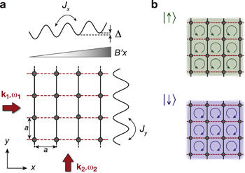
Figure 10. Experimental setup. (a) The setting consists of a square lattice with constant a = λs/2 and tunnel couplings Jx,y. A magnetic field gradient  generates a linear potential with magnitude Δ between neighboring sites. For Δ ≫ Jx the dynamics along x is frozen and resonantly restored again with a pair of running-wave beams (red arrows) with wavevectors
  and ω = ω1 − ω2 = Δ/ℏ. This generates the respective Peierls phases. (b) Two pseudo-spin components
  and
and  , which denote two different Zeeman states with opposite magnetic moment, will see an artificial field that depends on the spin of the particle: Φ↑ = π/2 and Φ↓ = −π/2. This dependence is caused by the magnetic field gradient, which gives rise to a spin-dependent linear potential ±Δm. Reprinted by permission from Springer Nature: [51] © Springer International Publishing Switzerland 2016.
Download figure:
Standard image High-resolution imageIn principle the linear potential could be also generated using optical dipole forces [124], which have the practical advantage that they are well-controlled, which offers an increased experimental flexibility. The scheme presented in this tutorial, however, is based on large energy offsets Δ. To reach this regime with optical potentials high-power or even near-resonant laser beams become unavoidable, which may cause severe heating due to spontaneous scattering of photons. Magnetic field gradients on the other hand allow for a large tuning range, while maintaining an almost perfect homogeneity of the potential over the extent of the atomic cloud. Moreover the magnetic field gradient offers a natural extension to realize TR invariant topological models, such as quantum spin-Hall systems [12, 13, 142].
6.1. Harper–Hofstadter model
Resonant tunneling is restored in the static lattice using two running-wave beams as discussed in the previous section (figure 10(a)). The two interfering beams create a local optical potential as defined in equation (64). In the high-frequency limit, the time-dependent problem can be mapped onto a time-independent one as discussed in section 3.4. The corresponding Hamiltonian can be written as

with  ,
,  ,
,  ,
,  . This Hamiltonian indeed mimics the physics of the Hofstadter model for α = 1/4.
6.2. Spin-dependent Harper–Hofstadter model
By exploiting an additional pseudo-spin degree of freedom the experimental configuration can be naturally extended to a TR symmetric topological Hamiltonian that underlies the quantum spin-Hall effect [12, 13]. The simplest version of a quantum spin-Hall insulator can be viewed as two independent copies of a QH insulator, where each spin state ( and
and  ) exhibits a magnetic field of the same strength but pointing in opposite directions depending on the state.
With cold atoms it can be realized by using two different states with opposite magnetic moments [41]. Here, we use two hyperfine states of 87Rb to encode the pseudo-spin, which are denoted as  and
and  .
.
The magnetic field gradient automatically generates a spin-dependent linear potential Δm = ±Δm, where the plus-sign corresponds to  and the minus-sign to
  particles. In section 3.1 we have shown that the Peierls phases ±ϕm,n depend on the sign of the energy differences ±Δ between neighboring sites and we find the effective Hamiltonian

where  and
and  is the z-component of the Pauli spin matrix
  . Without loss of generality we have neglected an additional π phase shift between the two spin-components, which has not effect on the properties of the system, since the two components are not coupled. It is easy to see that Hamiltonian (77) is TR symmetric and indeed describes two independent Harper–Hofstadter models, where Φ↑ = π/2 and Φ↓ = −π/2. Including additional terms in the Hamiltonian to couple the two individual components may indeed enable the study of non-Abelian gauge fields [143, 144].
6.3. Probing the magnetic flux distribution
In section 5.3 we have seen how superlattice potentials can be used to study the dynamics of single atoms in isolated plaquette potentials and how to extract experimentally the value of the artificially generated magnetic flux [92, 114]. In particular, the motion of the particle was found to be reminiscent of classical cyclotron orbits of charged particles in external magnetic fields. We have studied the micro-motion and its effect on experimental observables. Surprisingly, the results can be interpreted by considering the effective Floquet Hamiltonian in the rotating frame based on equation (72) since the micro-motion and the initial phase can be safely neglected for these measurements. In this section we are going to discuss how the same observables can be used to study the flux distribution across the lattice and the spin-dependence of the field.
As before the experiments were performed in a 3D optical lattice that consists of an array of isolated plaquette potentials (figure 9(a)). The final lattice depths were chosen such that the couplings within the plaquette were Jx/h = 1.2(1) kHz and Jy/h = 0.50(2) kHz and negligible coupling between neighboring plaquettes. Tunneling along x was suppressed by a magnetic field gradient of strength Δ/h ≃ 4.5 kHz.
The measurements started by preparing single atoms in the ground-state of the tilted plaquettes:  or
or  depending on the spin state. After suddenly switching on resonant coupling with K/h ≃ 0.28 kHz the mean atom position was measured as a function of time. All plaquette parameters Δ, J and K were calibrated independently for each measurement. A detailed description of these calibrations and further details about the experimental sequence can be found in [41, 51]. Using the site-resolved detection technique mentioned earlier [125, 126] we evaluated the mean atom positions
  and
and  within the plaquettes. Here we measured Nleft = NA + ND, Nright = NB + NC, Nup = NC + ND and Ndown = NA + NB, since it is technically more demanding to measure all
  at once.
We observe that once tunneling is restored the atoms start to tunnel to the opposite bond. Due to the gauge field, however, they get deflected along y, perpendicular to their initial velocity (figure 11). We observe that both spin components are deflected in the same direction, hence, the chirality of their cyclotron-like motion is opposite for the two spins as expected for a magnetic flux, whose direction depends on the spin Φ = ±π/2.

Figure 11. Quantum cyclotron orbits obtained from the mean atom positions  and
and  for J/K ≈ 2. The gray solid lines display the fit of the expected evolution X(t) to the data. The curve was calculated based on the effective Hamiltonian (72) for the independently calibrated parameters J, K and Δ. In addition the flux was set to Φ = 0.73(5) × π /2 (section 5.3) and a small time delay of τ = 0.12(5) ms was introduced. The remaining free fit parameters were the offsets and oscillation amplitudes,
  and
and  , along the two axes. The schematics illustrate the optical and magnetic potentials, initial states for
  (green) and
  atoms (blue) and the direction of the flux. For (b) the superlattice along x was shifted by one lattice constant compared to the one in (a) in order to demonstrate the uniformity of the flux distribution. Every data point was evaluated from three individual experimental realizations. For clarity error bars are not displayed but can be found in [41]. Reprinted figure with permission from [41], Copyright (2013) by the American Physical Society.
Download figure:
Standard image High-resolution imageThese measurements alone cannot distinguish a staggered flux distribution Φ = (−1)m π/2 from a uniform one because only plaquettes with equal sign of the flux contribute to the signal (section 5). However, by shifting the superlattice potential by one lattice constant (figure 11(b)), for instance, along the x-axis, one can select a different set of plaquette potentials, which have not participated in the previous measurements. We performed equivalent measurements in this configuration and observed exactly the same chiralities for the two spin components as before, which is a signature of the uniformity of the generated flux distribution.
The measured mean atom position  along x, was fitted according to
  , where X(t) was computed using the effective time-independent Hamiltonian (72), X0 and
  were free fit parameters and we have introduced a small experimental time delay τ, which is caused by finite ramp durations. It is not know a priori but it was calibrated and held constant in the fitting algorithms. For the calculation we used the previously determined value of the magnetic flux per plaquette Φ = 0.73(5) × π/2 (section 5.3), whose reduced value stems from the smaller distance between lattice sites along y in the superlattice potential [92].
6.4. Spin-Hall effect in an optical lattice
The spin-Hall effect is closely related to the usual Hall effect, with the difference that in this case a transverse spin current develops if a potential difference is applied to the material. There is no net charge current because spin-up and spin-down electrons are deflected in opposite directions. As a result a transverse spin imbalance builds up, which is analog to the transverse Hall voltage in conventional Hall systems. Experimentally the spin-Hall effect has been studied wit thin-film semiconductor devices [145, 146] and was simulated with harmonically trapped neutral atoms using Raman dressing [147].
Here we briefly review the first experimental study of spin-Hall physics with cold atoms trapped in optical lattices [41]. Based on the previous measurements we study the dynamics of single atoms in plaquette potentials as a function of the spin imbalance  , where ni = Ni/N, i =
  is the fraction of atoms in one spin component. We focus on the analysis of the dynamics in the non-trivial direction, i.e. perpendicular to the initial direction of motion. The experimental sequence was similar to the one described in section 6.3, but this time the atoms were initially prepared in a spin-superposition state
  before they were prepared in a superposition state on the lower bond of the plaquette potential, with equal weight on A and B sites independent of the spin
  of the particle (insets in figure 12). This was achieved by setting the tunneling along y to a small value during state preparation. Increasing it suddenly to a larger value then initiated the dynamics and we measured the mean atom position in the non-trivial x-direction
  . Details of the experimental sequence are described in [41]. We found almost perfectly mirrored oscillations for the two spin components and extracted the oscillation amplitudes by fitting the numerical evolution as explained above. We found
  for
for  (blue) and
  for
for  (green). In figure 12 we display the measured spin-dependent amplitudes as a function of spin imbalance
  . We observe a linear dependence with a sign reversal when the spin is flipped, as expected for the spin-Hall effect.

Figure 12. Oscillation amplitude as a function of the spin-imbalance. The oscillation amplitude  was evaluated by fitting the evolution expected from Hamiltonian (72) to the measured mean atom position
  using the independently calibrated parameters J/h = 0.69(1) kHz, K/h = 0.38(1) kHz, Δ/h = 5.31(5) kHz, Φ and a small time delay of τ = 0.18(3) ms. Every data point is averaged over two experimental realizations. The insets illustrate the initial state and the sign of the flux for a spin-polarized sample:
  (blue) and
  (green). The solid line is a linear fit to the data, where the offset was set to zero. The error bars depict the standard deviation obtained from the individual measurements. Reprinted figure with permission from [41], Copyright (2013) by the American Physical Society.
Download figure:
Standard image High-resolution image7. Chern number measurement
In section 2.4 we have introduced the topological properties of the Hofstadter model and in the previous section we have demonstrated that such a model can indeed be realized using the laser-assisted tunneling technique introduced in section 3.3. Here, we are going to present an short overview of the first measurement of the non-trivial Chern number of an artificially generated Hofstadter system with ultracold atoms via the observation of bulk topological currents [73, 148, 149].
7.1. Experimental setup and preparation sequence
The experimental setup was modified compared to the one described in section 6 in order to increase the experimental flexibility in designing an adiabatic preparation sequence. We have developed an all-optical scheme as illustrated in figure 13(a). The key difference is that one of the running-wave beams is now retro-reflected to create a standing wave, which enables a spatial addressing of every other bond in the lattice. In order to address the remaining ones, the setup needs to be doubled, facilitating flux rectification in a staggered superlattice, which otherwise would result in a staggered flux distribution.

Figure 13. Realization and properties of the Hofstadter model for α = 1/4. (a) Illustration of the experimental setup, which consists of a static square lattice with a staggered energy offset Δ ≫ Jx to inhibit tunneling in the x-direction. Two additional pairs of beams (red and blue arrows) restore resonant tunneling along that axis for ωi = ωi2 − ωi1 = ±Δ/ℏ. (b) Schematic drawing of the effective Floquet Hamiltonian with uniform flux Φ = ±π/2 realizing the Hofstadter model for α = 1/4. The experimental parameters were adjusted to obtain equal tunnel coupling J = 75(3) Hz along both axes [V0/(ℏω) = 0.58(2)]. The green shaded area indicates the magnetic unit cell, which contains four non-equivalent sites (A, B, C, D). (c) The corresponding energy spectrum displays three well-separated subbands with Chern numbers νμ = {1, −2, 1} (section 2.4), Egap ≃ 1.5J denotes the lowest bandgap and Ebw ≃ 0.2J the bandwidth of the lowest band. Adapted by permission from Macmillan Publishers Ltd: Nature Physics [73], © 2015 Macmillan Publishers Limited. All rights reserved.
Download figure:
Standard image High-resolution imageThe basic operating principle is as follows: along the x-axis tunneling is inhibited by a staggered superlattice potential of the form  , with alternating energy offset ±Δ and hopping Jx between neighboring sites whose strength is determined by Vl and Vs. Tunneling is then resonantly induced using two pairs of laser beams (red and blue arrows in figure 13(a)), with frequency differences
  , i = {r, b}. Both pairs create time-dependent potentials of the form
  , with kR = ks/2 = π/(2a). Independent control over tunneling on bonds with energy offsets of the same sign (red and blue bonds in figure 13(a)) is obtained for ξ = π/4. In this configuration the red pair of beams induces tunneling only on the red bonds and the blue pair on the remaining ones. Setting
  realizes a uniform flux Φ = ±π/2 per plaquette (figure 13(b)).
In the high-frequency limit ℏω ≫ Jx,y the system can be described by the Hofstadter model for α = 1/4. A detailed derivation of the effective Hamiltonian in the experimental gauge including the effect of the initial phase, which introduces additional corrections, can be found in [51]. The lattice parameters were set to have equal effective coupling strengths along both axes.
Following the theoretical description presented in section. 2 we find that the magnetic unit cell is four times larger than the lattice unit cell AMU = 2a × 2a. It contains four non-equivalent sites and the lowest tight-binding band splits in into four subbands, where the two middle ones touch at four Dirac cones (figure 13(c)). Hence we speak of three well-separated Hofstadter bands. The lowest band exhibits topological properties equivalent to the lowest Landau level, with Chern number ν1 = +1. Moreover it is characterized by a rather large flatness ratio of Egap/ Ebw ≃ 7 making this system an excellent candidate to study fractional Chern insulators [150].
Having generated the desired bandstructure leaves one with the non-trivial task of preparing the atoms in the lowest Hofstadter band. Let us consider a sequence where we start with a BEC in the lowest band of the static trivial square lattice. Turning on the artificial flux immediately leads to a splitting of the band and the atoms might distribute between the higher Hofstadter bands in an uncontrolled way. To overcome this challenge we designed an alternative sequence, where we use additional staggered potentials along both directions to increase the unit cell of the static lattice. It is of the form

Turning on the modulation for large enough δ does not induce tunneling and the system remains trivial. Tuning the parameter δ allows us to connect these trivial bands to the Hofstadter bands in a controlled manner, since the number of subbands remains constant. The Hofstadter model with α = 1/4 is reached for δ = 0. Here we benefit from the increased experimental control facilitated by the all-optical setup [73].
The sequence started by preparing a BEC in the static lattice, which has a unit cell equivalent to the magnetic unit cell of the final configuration as depicted in figure 14(a). This is achieved with the additional staggered potentials, which introduce a detuning such that the laser-assisted tunneling is off-resonant. In the x-direction the detuning increases the already existing energy offset away from the resonance condition to Δ + δ, while along y it inhibits normal tunneling for δ ≫ Jy. In this regime the bandstructure is topologically trivial but the unit cell has the same size as the final magnetic unit cell. By slowly decreasing δ to zero we connect the spectrum to the desired Hofstadter spectrum (figure 14(b)). As a consequence, the number of bands is preserved during the loading sequence. It starts with large detuning (δ > 2J) with trivial bands, whose Chern numbers vanish. By decreasing δ one crosses a topological phase transition at δ = 2J, where the gaps in the spectrum close. Beyond this point the system is topologically non-trivial with non-zero Chern numbers and at the end of the sequence (δ = 0) the Harper–Hofstadter Hamiltonian for Φ = π/2 is realized, whose lowest band is characterized by ν1 = +1. When crossing the topological phase transition the gaps in the spectrum close at one point in the FBZ (figure 14(b)). However, if we prepare a BEC in the lowest band it should be only minimally affected by this gap-closing point.
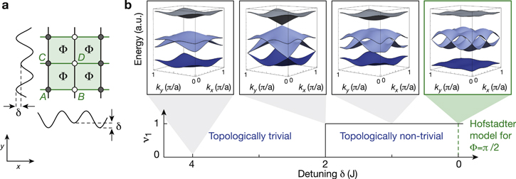
Figure 14. Energy spectra and topology of the Bloch bands for different staggered detuning values. (a) Schematic drawing of the Hofstadter lattice with equal detuning δ along both axes. Its unit cell is illustrated with the green shaded area, which contains four non-equivalent lattice sites (A, B, C, D). (b) Energy spectra as a function of detuning. For large detuning δ > 2J the bands are topologically trivial with vanishing Chern numbers. At δ = 2J there is a topological phase transition, where the gaps in the spectrum close and the system enters the topologically non-trivial regime with non-zero Chern numbers. For resonant tunneling (δ = 0) the bandstructure is equivalent to the one of the Hofstadter model with flux Φ = π/2. Note that the energy axis is rescaled for each spectrum. Adapted by permission from Macmillan Publishers Ltd: Nature Physics [73], © 2015 Macmillan Publishers Limited. All rights reserved.
Download figure:
Standard image High-resolution imageMoreover this protocol can be reversed, which allows us to map the population of the different Hofstadter bands onto four topologically trivial subbands in the static lattice and perform band-mapping measurements to determine the populations experimentally. Assuming that heating effects and scattering processes are negligible during this sequence we further obtain access to the momentum distribution of the Hofstadter bands. Using this technique we found that we achieve an initial atom population in the lowest Hofstadter band of about 60%.
7.2. Anomalous Hall velocity and Chern number measurement
In section 2.4 we have seen how in electronic systems the quantized Hall conductance relates to the Chern numbers of the occupied energy bands. A complementary way to describe the properties of QH insulators can be established by looking at boundary modes. A quantum Hall system is insulating in the bulk but conducting at the edges and the conductivity is given by the number of metallic edge states, which is in turn related to the sum of Chern numbers below the Fermi energy, known as bulk-edge correspondence [8, 9].
In many cold-atom experiments there are no steep potential boundaries in contrast to solid-state measurements, hence, it offers a natural setting to look for observables that study the bulk topological properties. Indeed it was shown that a measurement of the anomalous Hall velocity [72], that emerges transverse to an applied potential gradient and is proportional to the Berry curvature, could reveal the Chern number of the corresponding energy band [148, 149].
Using a semi-classical approach one can calculate the velocity of a wavepacket in a state  of the μth energy band centered around momentum k in the presence of an external force
  , according to [72]
As captured by the band velocity  , the wavepacket performs Bloch oscillations [123] but in addition it exhibits a transverse velocity component proportional to the Berry curvature Ωμ(k) defined in equation (20), which is the origin of the Hall velocity (figure 15(a)). Recently, the anomalous Hall velocity was observed with ultracold atoms in a shaken honeycomb lattice [40] and in an electronic graphene superlattice [151].
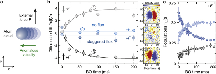
Figure 15. Differential transverse center-of-mass displacement as a function of the Bloch oscillation time. (a) Applying an external force to an atom cloud in a non-trivial bandstructure induces a perpendicular Hall drift, determined by the anomalous velocity  in equation (79). For a uniformly filled band the mean displacement is proportional to the sum of the Chern numbers νμ of the occupied band μ, which can be observed by taking in situ images of the atoms. (b) The black and gray data points show the transverse motion for opposite directions of the force
  (Fa/h = 38.4(8) Hz) for atoms prepared in artificial Hofstadter bands (Φ = π/2). The blue data points display the result of a similar measurement for topologically trivial bandstructures without magnetic flux Φ = 0 (light blue) or with staggered field Φ = (−1)mπ/2 (dark blue). Each data point is obtained from five datasets, the error bars show the corresponding standard error of the mean. The solid black and gray lines display a fit based on equation (86) and the independently measured filling factor γ(t) as obtained from the observed band populations ημ(t). The following Chern numbers were obtained:
  (black) and
  (gray). The blue solid lines are guides to the eye. Each of the panels on the right displays one averaged dataset for the experimental configurations indicated by the numbers. (c) Measured band populations ημ(t). The color code illustrates the connection to the different Hofstadter bands as in figure 13(c). Each data point consists of two measurements and the error bars denote their standard deviation. Adapted by permission from Macmillan Publishers Ltd: Nature Physics [73], © 2015 Macmillan Publishers Limited. All rights reserved.
Download figure:
Standard image High-resolution image
This anomalous component can be employed to experimentally determine the Chern number of an energy band of interest. To isolate the non-trivial dynamics from the band velocity components, one may consider a uniformly populated energy band, where the particle density ρμ(k) ≡ ρμ at a certain momentum k and hence per state  is independent of k. Due to the symmetry of the dispersion relation the contributions from the band velocity identically vanish. For an infinite system the mean band velocity for the μth band is computed as

where the integration is performed over all momenta in the FBZ. For fermions this is achieved, if the Fermi energy lies within a spectral gap [149]. Here we consider bosonic atoms, which naturally condense in the lowest energy eigenstate. However, if we consider a finite-temperature system, whose temperature is large compared to the bandwidth of the lowest band but small compared to the energy gap, one can realize an incoherent distribution of atoms which populate the band approximately uniformly. In both cases the mean anomalous velocity of the μth band of an infinite system is calculated as

where νμ is the Chern number of the μth band. For well-separated non-degenerate energy bands the particle density in each band is found according to

where Nμ is the particle number in each band,  is the total atom number and AFBZ = π2/a2 is the area of the FBZ. Under the assumption that no additional dynamics occurs that would change the band populations over time (ημ ≡ ημ0), one can compute the contribution of the μth band to the center-of-mass (COM) displacement of the atoms transverse to the applied force as follows

where τB = h/(Fa) is the Bloch oscillations period. For a filled lowest band η1 = 1 (ημ>1 = 0) we obtain x1(t) = −4aν1t/τB, which corresponds to a deflection of 4aν1 per Bloch oscillation period and the Chern number ν1 can be simply extracted from the slope of the linear displacement. It is at least on the order of four lattice constants and therefore can be detected with conventional imaging systems.
The initial state preparation is likely not perfect, hence there will be higher-band occupancies, which can be easily incorporated in the equation of motion. The Hofstadter model for Φ = π/2 consist of three energy bands. Note that the middle one consists of two subbands (figure 13(c)) and contains twice as many states. Thus, the particle density is determined by ρ2 = η2/(2AFBZ); for each momentum there are two available quantum states. The combined COM-displacement  is given by

Using the particle-hole symmetry of the Hofstadter model and  as discussed in section 2.4 this relation can be further simplified. Since the Chern number distribution is symmetric around zero energy one finds ν1 = ν3 = −ν1 − ν2, which can be used to rewrite equation (84) in terms of the lowest band Chern number:

where we have introduced the initial band-filling factor γ0, which was assumed to remain constant during the dynamics. The largest deflection occurs for γ0 = 1, which corresponds to a filled lowest band, while it continuously decreases if higher-band populations are taken into account. For an infinite temperature state, γ0 = 0 and no transverse motion is expected.
Finally the question on the importance of the micro-motion for the COM-measurement arises. In the high-frequency limit the dominant contribution to the micro-motion operator is defined in equation (54). We find that it is diagonal in the density operator  and we expect no influence of the micro-motion on our measurement. This lowest-order approximation is valid in the limit ℏω ≫ Jx, which is well fulfilled for the measurements discussed in the following section, where ℏω / Jx ≃ 13.5. For parameter regimes, where this limit is not well fulfilled additional contributions are expected that scale with an amplitude Jx/(ℏω) [102] as already discussed in section 5.3. For comparison, the residual oscillations shown in figure 9(c) for the cyclotron dynamics would be reduced by a factor of ∼3 for the experimental parameters used for the Chern number measurement.
7.3. Experimental results
The experimental sequence started by preparing the atoms in the Hofstadter bands using the loading scheme presented in section 7.1. Subsequently an external force F was applied. It was created using an additional laser beam, which was aligned along y, so that the atoms are positioned at the maximum slope of the Gaussian beam profile to induce the potential gradient, while along x the cloud was centered on the profile. We then tracked the COM-motion in situ using absorption imaging. In order to be less susceptible to systematic errors, that might be induced by a long-term drift of the absolute position of the atomic cloud, we measured the positions for opposite directions of the flux Φ = ±π/2 and evaluated the differential shift x(t, π/2) − x(t, −π/2) = 2x(t). In the following one dataset is defined as a set of ten images for each direction of the magnetic flux, which were taken in an alternating manner, averaged and then subtracted (figure 15(b) right column).
For short times there is an almost linear evolution of the differential COM-displacement in agreement with equation (85) and numerical studies [148, 149]. For longer times 2τB > 50 ms, however, we observe a rapid saturation of the transverse motion (figure 15(b)). Numerical simulations did indeed reveal small deviations from a perfectly linear evolution, which is due to Landau–Zener transitions. The observed saturation, however, happens on a much faster timescale. This suggests that additional effects associated with heating, most likely caused by the periodic modulation and its interplay with interactions between the particles, lead to repopulation between the bands [152, 153]. Moreover, we see a symmetric evolution with respect to the direction of the force  (black and gray data points) and no significant motion for a lattice without flux Φ = 0 (light blue data points) or staggered flux (dark blue data points), whose bands are topologically trivial with ν = 0 (section 5).
Making use of independent band population measurements we were able to confirm that atoms are transferred to higher Hofstadter bands during the dynamics, which induces a time-dependence for the filling factor γ(t) (figure 15(c)). This could be incorporated into our theoretical model by extending equation (85) and we obtain

with ![$\gamma (t)=[{\eta }_{1}(t)-{\eta }_{2}(t)+{\eta }_{3}(t)]$](https://content.cld.iop.org/journals/0953-4075/51/19/193001/revision2/jpbaac120ieqn206.gif) . The timescale associated with the decay of the filling factor
. The timescale associated with the decay of the filling factor  is consistent with the saturation of the observed COM-motion. Incorporating the additional population data in our model and fitting equation (86) to the COM-data enables a determination of ν1, where the Chern number is the only free fit parameter. With this we found νexp = 0.99(5) (averaged over four independent measurements), which is in agreement with the theoretically expected value. Indeed this demonstrates that we have a good quantitative understanding of the dynamics and properties of the Floquet-engineered bandstructure. However, in order to improve temperatures by suppressing the heating mechanisms more detailed studies on modulation-induced heating processes are required [152, 153].
8. Summary and conclusion
We have reviewed several experimental results that underline the power of Floquet engineering for the design of quantum systems with novel properties [39, 119] in particular those that rely on resonant laser-assisted tunneling. The main results include the study of staggered magnetic fields and the observation of cyclotron-like dynamics of neutral particles [92, 114], which further demonstrated future possibilities to study quantum spin-Hall systems or non-Abelian gauge fields via the realization of spin-dependent fields [41]. Moreover, we have discussed different implementations of the Hofstadter model [41, 51], a paradigmatic topological lattice model, where we adiabatically prepared a cold cloud of atoms in the lowest band for a flux α = 1/4 and performed transport measurements, which revealed the Chern number and hence the topological properties of the lowest energy band [73]. Up to date most of the experimental studies have focused on the single-particle dynamics in engineered bandstructures and it is of particular interest to extend these studies to the many-body regime in the near future. In order to access this regime several experimental and theoretical questions have to be addressed.
One such challenge consists in the severe heating that some of the experiments have reported, which increases with increasing interaction strength. While single-particle scattering effects are well understood and have been studied experimentally [154], we still lack a complete understanding of collision-induced heating in Floquet systems [152, 153, 155–163]. Very recently a first experimental study on collision-induced heating mechanisms in driven bosonic 1D lattices was presented [164], which confirmed predictions based on a Floquet Fermi Golden rule (FFGR) approach. Such processes could be suppressed, for instance, in 3D lattices where the number of available scattering modes induced by the transverse degrees of freedom in a 1D lattice, is decreased [152, 160, 165]. First experiments reported promising results in 3D systems [166], however, more detailed studies are required in the future. FFGR work successfully in the long-time limit, where incoherent two-body scattering dominates. The origin and onset of instabilities at short times is however driven by coherent dynamics. Recently theoretical studies have investigated these dynamics for weakly-interacting BECs in driven optical lattices predicting parametric instabilities whose existence could be readily observed in TOF experiments [167, 168].
Acquiring a good understanding of interaction-induced heating in Floquet systems, will allow for the engineering of intriguing strongly-correlated states in driven systems, which may enable studies of topological many-body phases such as fractional Chern insulators [11, 150]. The artificial Hofstadter bandstructure constitutes a promising starting point to realize such states in the laboratory [68–71]. Further challenges are associated with suitable experimental observables to study the exotic properties of topological many-body states, which might be envisioned as extensions of available experimental probes for the single-particle regime [110, 169–171]. Moreover there is a strong need for designing quench protocols to gain new observables [172] and adiabatic preparation schemes for topological many-body states [173, 174].
An alternative pathway to first studies of interesting many-body phases in the presence of artificial magnetic fields could be the generation of interacting ladder systems. It has been shown, that this quasi-1D geometry is well suited to study the effect of gauge fields in a setting that can be nicely handled experimentally and numerically and allows for benchmark results that will be important for more complicated studies in 2D systems. Previously, this system facilitated the observation of Meissner-like chiral currents [115] and several theoretical studies reported exotic strongly-correlated phases [175–182]. In combination with high-resolution microscopes [136–141] this opens a panoply of exciting new possibilities to investigate topological many-body physics using the well-controlled setting of ultracold atoms in optical lattices.
Acknowledgments
I thank the experimental teams of I Bloch at the Ludwig-Maximilians University of Munich and the Max-Planck-Institute of Quantum Optics in Garching for their support and help regarding scientific, practical and administrative matters. In particular I want to thank my supervisor I Bloch for his great support. Special thanks goes to M Atala, J T Barreiro, Y-A Chen, M Lohse, S Nascimbène, C Schweizer and S Trotzky for the joint experimental work on topological systems with ultracold atoms in optical superlattices. We also had many fruitful discussions and theory collaborations, in particular I would like to thank D Abanin, M Burrello, N Cooper, J Dalibard, E Demler, N Goldman, F Grusdt, T Kitagawa, L Mazza, B Paredes and O Zilberberg. I further acknowledge support from the Deutsche Telekom Stiftung, the European Commission (UQUAM grant no 319278) and the Nanosystems Initiative Munich (NIM grant no. EXC4).