

Abstract
We present a microfluidic device which allows one to study the dynamics of oscillatory flows for a frequency range between 1 and 300 Hz. The fluid in the microdevice could be Newtonian, viscoelastic, or even a biofluid, since the device is made of PMMA, which makes it biocompatible and free of elastomeric elements. Coupling a piezoelectric to a micropiston allows one to impose periodic movement to the fluid, with zero mean flow and amplitudes of up to  m, within the microchannels in which the dynamics is studied. The use of a fast camera coupled to a microscope allows one to study the dynamics of
  m tracer particles and interfaces at an image acquisition rate as fast as 5000 frames per second. The fabrication of the device is easy and cost-effective, since it is based on the use of a micromilling machine. The dynamics of a Newtonian fluid is studied as a proof of principle.
Export citation and abstract BibTeX RIS
1. Introduction
Microfluidic devices are useful for countless applications in chemical and biochemical analysis, biomolecular separation and micromixing, to mention a few [1–7]. Microfluidics aims to integrate many functions on a single lab-on-a-chip device for technological applications in physics, material sciences, biology and medicine [8–12]. It does this by the integration of micro-scale pumps, filters, sievers, valves and sensors within the microfluidic channels. The study of pulsatile flows can be used to analyze optimal flow conditions, since the fluids' responses are different for different frequencies of the imposed pressure gradients [13–18], and to control and optimize existing processes. In microfluidics, pulsatile flows can lead to the conception of new devices for manipulation, separation, mixing, analysis and characterization of surface properties [19, 20].
Pulsatile flow in microfluidics has been extensively addressed in the context of valveless micropumps. A vibrating diaphragm coupled with a nozzle–diffuser geometry is among the most popular configurations of such devices [21–27]. A piezoelectric actuator causing the vibration of a membrane is an excellent option to impose periodic movement to a fluid [28]. However, the coupling of a piezoelectric actuator to a vibrating membrane and to the micrometric channels is not straightforward, and a combination of different materials and complicated fabrication methods has usually been necessary.
In the present work we present a microfluidic device, which we refer to as a microfluidic flow spectrometer (MFS), made exclusively of PMMA, which can be easily coupled to a piezoelectric ceramic to create periodic flow with zero mean. We do this by means of micromilling, which is an easy and cost-effective fabrication method [29]. Our device has the advantage of being made of a single rigid material, in contrast with soft elastomeric materials used in microfluidics such as PDMS. The lack of elastic materials in our device is important because, in principle, it allows one to study the elastic properties of viscoelastic fluids without interference from the elasticity of the device.
We first present in detail the fabrication of the device. Next we present the experimental setup and the methods necessary to impose a periodic signal to a fluid within the microchannels; we then use the MFS to study the pulsatile dynamics of a Newtonian fluid as a proof of principle. Finally we show that, with the MFS, it is also possible to study the dynamics of interfaces.
2. Fabrication and characterization
Two 1.5 mm thick, acrylic wafers are drilled with an MDX-40A milling machine (Roland) using a 0.8 mm, two-flute carbide end mill according to the pattern shown in figure 1(a). A central circular pool and two lateral microchannels are drilled on the lower wafer. The lateral microchannels have a 1 mm width and  m depth rectangular cross section. The central pool has a depth of
  m and a diameter of 4 mm. The top side of the upper wafer is drilled (in the light-color area shown in figure 1(a)) to obtain a
  m-thickness ring-shaped membrane with a central column (piston). Owing to its small thickness, the membrane will be deformable despite been made of PMMA. The external diameter of the ring (on the upper wafer) is equal to the diameter of the pool (in the lower wafer) so that, when the two wafers are glued, the flexible membrane covers the pool.
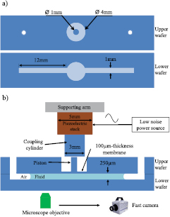
Figure 1. Schematic representation of the experimental setup. (a) Top view of the upper and lower PMMA wafers before gluing them together. (b) Lateral central cross section of the device with the PMMA wafers already glued, showing the piezoelectric stack coupled to the PMMA device, through a coupling cylinder. The fluid of interest, partially filling the microchannels, is also depicted. The displacement of the piezoelectric stack is controlled by a low-noise power source, under sine wave generation mode. The observation zone of the tracer particle is at a midpoint between the central pool and the fluid–air interface. A fast camera is used to record images as fast as 5000 frames per second.
Download figure:
Standard image High-resolution imageThe positioning of the end mill in the vertical direction has a resolution as precise as  m, so making a membrane with a thickness of a hundredth of a micrometer does not present a problem.
To amplify the effect of a piezoelectric on the membrane, we glue together two identical piezoelectric transducers (TA0505D024, Thorlabs, Inc.). We call this array a piezoelectric stack. The top side of the piezoelectric stack is fixed to a supporting arm, and the bottom side is glued to a 3 mm diameter PMMA (coupling) cylinder, that has a diameter smaller than the external diameter of the ring. Before starting an experiment, we make the coupling cylinder (glued to the piezoelectric stack) approach the piston of the PMMA device by moving the supporting arm with the help of a micrometric screw. Once the coupling cylinder and the piston are in contact, we apply an external voltage that causes the piezoelectric stack to deform, which in turn causes vertical displacement of the membrane (see figure 1(b)).
The geometry of a large central pool connected to the small lateral microchannels allows one to amplify small displacements of the fluid in the pool into large displacements of the fluid inside the microchannels. For instance, in our device a  m-vertical displacement of the piezoelectric stack and the membrane above the pool represents a fluid displacement of about
  m in the central part of the microchannels.
We choose the width of the microchannels (1 mm) much larger than their depth ( m) so that the flow profile in the central part of the microchannels, far from the lateral walls, should be similar to a two-dimensional flow profile, which is known analytically. However, our fabrication method allows us to adjust the width–depth ratio as desired, with the minimum possible width determined by the minimum size of the end mill (
 m for our machine).
The method used to bond the two wafers is easy, fast and very effective; it was conceived and described by Ogilvie et al [30]. Briefly, the acrylic wafers are thoroughly cleaned after micromilling and exposed to chloroform vapor for 4 min. Then they are pressed together, first by hand (1 min), and then in a hot press by applying pressure (∼150 N cm−2) and heat (65 °C) in a controlled and uniform way for 30 min. Not only is this method effective in terms of bonding strength (∼3 N mm−1), it also has the advantage of reducing the excessive roughness of the microchannels which results from drilling, making them transparent to the optical microscope [30]. However, the roughness is not completely suppressed and it can be clearly appreciated in figure 2(a), in the left portion of the microchannel (that is not filled with liquid). In contrast, the same figure shows that in the right portion of the microchannel (filled with liquid), the roughness of the microchannel is less obvious, due to the similarity in refraction indices of the liquid and the PMMA. This greatly improves the optics and allows the filming of tracer particles. At a magnification of  it is possible to visualize the whole width of the microchannel, and the liquid–air interface can be clearly distinguished. This is useful because interface dynamics is interesting for the microfluidics community, although we do not study it in depth in this work. In figure 2(a) the magnification is enough to see the whole interface but it does not allow one to distinguish tracer particles. In order to have a good image of these it is necessary to use a
  microscope objective with a
  augmentation. Figure 2(b) shows a 1μm tracer particle focused in the middle of the microchannel using such a magnification (for the image of the figure, an extra digital zoom was used). From these kinds of images, taken at thousands of frames per second, it is possible to obtain the position of the particle as a function of time, and therefore the displacement of the fluid in the neighborhood of the particle.
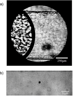
Figure 2. (a) Image of the liquid–air interface inside a 1 mm wide microchannel acquired using a magnification of  and focused at the center of the microchannel with respect to the top and bottom borders. The roughness of the microchannel is evident in the air side. The fluid (glycerol at 70%) improves the optics because of the similarity between the refraction indices of both materials. (b) A 1
  m tracer particle in the same microchannel with a
  microscope objective with an additional
  augmentation. The image is shown with an extra digital zoom.
Download figure:
Standard image High-resolution imageIn an independent setup, we characterized the elastic properties of the membrane (within the two glued wafers) by applying different over (and under) pressures and observing the membrane displacements. The pressure was applied by sealing the space above the membrane (and piston) with a PMMA lid, to create a chamber connected (with a plastic tube) to a valve, that switches between a compressor and a vacuum pump. The value of the displacement was obtained by filling the pool with water mixed with fluorescein and measuring the intensity of fluorescence in each pixel of an image of the bottom of the pool. The intensity of fluorescence in each pixel is proportional to the height of the column of liquid above it. By measuring the relation between the intensity of fluorescence and the height of the column in another setup, for which the height of the column is known, it is possible to obtain a good estimation of the displacement of the membrane at different pressures. Figure 3(a) shows the displacement of the membrane as a function of radial position for different values of the pressure. In figure 3(b), we plot the applied pressure as a function of membrane displacement at its center. It can be noted that the elastic behavior of the membrane is in the linear regime, and a Hookean stiffness constant equal to  N m−1 can be obtained from the data.
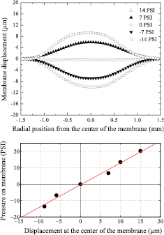
Figure 3. (a) Displacement of the membrane as a function of the radial position for different values of pressure. (b) Applied pressure as a function of displacement at the center of the membrane. From these data it is possible to obtain a Hookean elastic constant of the membrane, equal to  N m−1.
Download figure:
Standard image High-resolution imageThe piezoelectric stack produces a displacement of the membrane proportional to the applied voltage. The maximum value of the membrane displacement in our experiments is  m, due to the maximum peak-to-peak voltage of 50 V recommended in the datasheet of the piezoelectric transducers. This value is small compared to the maximum possible displacement that the membrane could have (see figure 3(b)). Therefore, the dynamics of the membrane at such amplitudes is expected to be linear and symmetrical with respect to the equilibrium position. In the linear regime the natural frequency of the membrane can be estimated as the square root of the ratio between the stiffness constant, κ, and the mass of the membrane (and piston). Since the density of PMMA is 1200 kg m−3, the natural frequency of the membrane is approximately 15 kHz. This frequency is far beyond those used to drive the fluids in this work, so it does not interfere with the dynamics of the fluid studied.
3. Experimental setup
The microfluidic device is made of PMMA and it consists of two long lateral microchannels and a central pool above which a  m thick membrane moves up and down, creating a periodic flow in the microchannels; see figures 4(a) and (b). The height of the lateral microchannels and the pool is
  m and the width of the lateral microchannels is 1 mm. The fluid completely fills the pool while the total length of the microchannels is only partially filled. This configuration is stable because, given the small dimensions of the microchannels, capillary forces are strong enough to keep the fluid confined. The advantage of working with microchannels that are only partially filled is that we avoid the strong geometrical variations that would occur if the microchannels were connected to external tubes. This is important because in pulsatile flows geometric asymmetries could lead to an effective pumping which we want to avoid [28]. Besides, pressure changes can be delayed in time in dynamic situations in the presence of abrupt geometric changes [31].
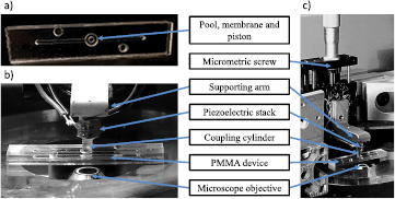
Figure 4. (a) Top view of the PMMA device ready to be used (with the two drilled wafers glued together). The two microchannels, the pool and the membrane with the piston—which will be in contact with the coupling cylinder—can be clearly seen. The two circles next to the microchannels are marks used for alignment of the two wafers. (b) Image of the PMMA device placed above the inverted microscope. The top side of the piezoelectric stack is fixed to a supporting arm, and the bottom side is glued to the coupling cylinder. Once the coupling cylinder and the piston of the PMMA device are in contact, the action of the piezoelectric stack on the PMMA device vertically displaces the membrane. (c) Zooming out on the setup shows that the supporting arm is attached to a micrometric screw which allows for precise positioning between the coupling cylinder and the PMMA device.
Download figure:
Standard image High-resolution imageA low-noise power source (Agilent Tech.), under sine wave generation mode, supplies the piezoelectric stack with a voltage waveform. The membrane above the pool is moved by the action of the piezoelectric stack, through the coupling cylinder and the piston of the PMMA device; see figure 4(b). The frequency range employed is 20–300 Hz, although the device can be driven at lower and higher frequencies.
The setup is placed above an Eclipse Ti Nikon inverted microscope with a  objective with a
  augmentation; see figure 4(c). Recordings are made on the lateral microchannels using a Photron SA3 high-speed camera (Photron Ltd.) at 5000 frames per second.
A solution of  glycerol in water was studied. This solution has density and viscosity equal to
  kg m−3 and
  cP respectively. These values were measured at
  C, which is the same temperature at which the experiments were performed. Tracer particles were incorporated into the fluid by adding few microliters of a dilution of 1 μm polystyrene particles in the same fluid, giving a final concentration of
  .
.
Particles located at the center of the microchannels (see figure 2(b)) were tracked by performing image analysis, from which the position as a function of time was obtained. This was done for different applied frequencies. The data for the position as a function of time were further processed in different ways as explained below.
4. Dynamics of pulsatile Newtonian fluids
We fill the microchannel with a Newtonian fluid, which consists of a mixture of  glycerol in water. We seed the fluid with tracer particles of
  m as described in section 3. We drive the fluid with different frequencies and record the position of a tracer particle (see figure 2(b)) half way along the microchannel's width and height, and half way between the extreme of the microchannel close to the pool, and the viscous fluid–air interface. We call h(t), the position of the particle along the flow direction from an arbitrary origin. A typical curve of h(t) shows the frequency imposed by the driving plus noise. Figures 5(a) and (b) show the raw data for the position of a tracer particle recorded for a typical experiment (in blue) for three different time windows, and the low-frequency overall behavior of the data,
  (in pink) for two of them (figures 5(b) and (c)). Figure 5(a) also shows a few images to illustrate the position of the tracer particle during one cycle.
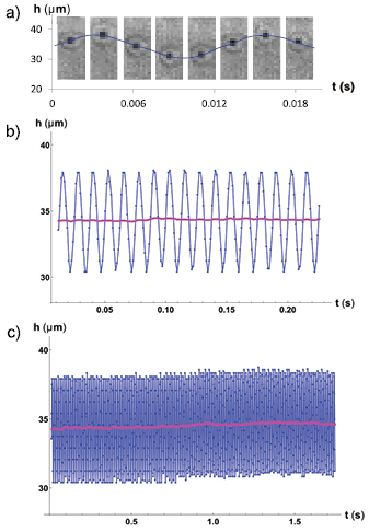
Figure 5. (a) Sequence of images of a tracer particle during one cycle of oscillation at  Hz. The blue line with dots corresponds to the positions of the particle determined from image analysis. The image acquisition rate for this experiment was faster than the sequence of images shown here, which is why the line has more points than images. (b) and (c) Raw data, for different time windows, of a tracer particle position as blue dots, and the low-frequency overall behavior of the same data as a pink line. The data correspond to an experiment at driving frequency
  Hz.
Hz.
Download figure:
Standard image High-resolution imageWe are interested in the dynamics of the fluid imposed by the piston. We therefore substract the low-frequency dynamics by defining  . A typical curve for h*(t) can be seen in figure 6, where the black dots correspond to experimental measurements, and the continuous line in red is the best sinusoidal fit to the data.
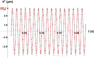
Figure 6. A typical curve for the tracer particle position h*(t) as a function of time. The time scale has been chosen in order to appreciate the frequency of the driving. On the vertical axis, the amplitude of the best sinusoidal fit to the data is shown as  . The data correspond to a driving frequency
  Hz.
Hz.
Download figure:
Standard image High-resolution imageThe dynamics of h*(t) can also be explored in the frequency domain, which displays explicitly a lot of information. A typical curve of the magnitude of the Fourier transform of the particle position,  , can be seen in figure 7. From this, it is clear that the main component of the dynamic signal is the driving frequency imposed by the piezoelectric,
  , but that there are other modes that compose the signal, both of lower and higher frequencies than that of the driving, including its harmonics.
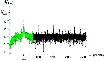
Figure 7. A typical curve for the magnitude of the tracer particle position  in the frequency domain. The main peak composing the signal is centered around the frequency of the driving,
  . The truncated signal which is used to obtain the distributions of velocity fluctuations, as explained in the text, is shown in a lighter color.
Download figure:
Standard image High-resolution imageTo compute velocities, we use the time-domain data for h*(t), namely,  . In order to obtain the best fit to the velocity data, we take the best sinusoidal fit h*(t) (illustrated in figure 6) and derive it analytically in time to obtain
  . This gives a cosine wave with amplitude,
  , for the best fit to the velocity data.
Figure 8 shows how the amplitude of the best fit to the velocity data changes with the Womersely number [32, 33]. This is proportional to the square root of the driving frequency, and inversely proportional to the square root of the characteristic viscous frequency of the confined fluid. It is defined as  , where the characteristic viscous frequency of the confined fluid,
  , is given by the viscosity and density of the fluid, and the characteristic length of the system, a, through the relation
  . We have chosen the characteristic length, a, as the hydraulic radius of the microchannel, a = WH/(W + H), where W and H are the microchannel width and depth, in accordance with the literature on pulsatile fluids in rectangular channels [33]. It is clear that glycerol at
  follows the piston movement up to about Wo = 1. This confirms the good quality of the piston movement, at least in the corresponding frequency range [20–190] Hz. It also shows that, in this frequency range, the movement of the piston is transferred directly to the fluid. For Wo > 1, theory predicts that pulsatile velocity profiles are no longer parabolic, but present off-center maxima. We therefore expect the magnitude of the velocity at the center of the microchannel to decay. Figure 8 shows that the amplitude of the best fit to the velocity data, at the center of the microchannel, decays for Wo > 1.
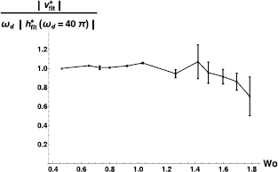
Figure 8. Amplitude of the best fit to the velocity as a function of the Womersley number. The velocity has been normalized by  . The amplitude at 20 Hz (
 ) corresponds to the lowest amplitude of our study.
Download figure:
Standard image High-resolution imageWe can also compute velocities in the frequency domain as  , which can be converted to the time domain by inverse-Fourier transforming
  . By taking the value of the maximum of the magnitude of the velocity in the frequency domain, at the driving frequency, and mapping it to the time domain, we have a second way of obtaining the amplitude of the velocity that corresponds to the driving-frequency mode. The data computed in this way (not shown), differ from the data shown in figure 8 by at most 2.4%.
In order to account for the dispersion of the data, we construct velocity distributions for v*. We show a typical velocity distribution in figure 9, and the distribution of an ideal cosine signal with dotted lines. For figure 9, we have normalized the velocity v* by the driving frequency,  , and the characteristic scale,
  . The analysis can also be done in the frequency domain, and in this case, the characteristic length scale would be
  (shown in figure 7) mapped to the time domain. These two length scales would be identical for a perfect one-mode signal.
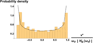
Figure 9. Distribution of velocities v* calculated in time domain. The data correspond to a driving frequency,  Hz. Typical distributions have roughly the characteristic shape of the distribution of a cosine wave, namely, two maxima at positive and negative large velocities, and a minimum around zero. The distribution of an ideal cosine mode is shown, for reference, with dotted lines. The velocities have been normalized by
  to deal with dimensionless quantities.
Download figure:
Standard image High-resolution imageTypical distributions obtained with both methods have the characteristics of the distribution of a signal dominated by a one-frequency mode, namely, two maxima around the maximum positive and negative values of the velocity, and a minimum around zero, as shown in figure 9.
Velocity fluctuations have proven to be non-Gaussian for the dynamics of a water front filling a hydrophobic microchannel with a low constant pressure difference along the flow direction [34]. The non-Gaussian nature of the distributions are due to the dynamics of pinning and avalanches of the contact line. In accordance with [34], we compute velocity fluctuations around an overall tendency by defining
where  . We compute the tendency by cutting high-frequency modes of the
  signal and multiplying this truncated signal (whose magnitude is shown in green in figure 7) by
  , to then inverse Fourier transform it to obtain
  in the time domain. Typical distributions for velocity fluctuations in our experiments are Gaussian, as can be seen in figure 10.
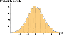
Figure 10. Distribution of velocity fluctuations around a tendency computed, in the frequency domain, by truncation of high-frequency modes (equation (1)). The data correspond to a driving frequency,  Hz. The distribution is clearly Gaussian.
Download figure:
Standard image High-resolution image5. Dynamics of pulsatile interfaces
The MFS can also be used to study interfacial dynamics. Figure 11(a) shows a snapshot of the interface between air and glycerol at 70% oscillating at 20 Hz. The image comprises the whole width of the microchannel (1 mm) and from image analysis it is possible to obtain the profile of the interface, which is shown in figure 11(b) for two different moments of the oscillation. Figures 11(c) and (d) show the position and velocity of the central part of the interface as a function of time, respectively.

Figure 11. (a) Image of the liquid–air interface in one of the microchannels taken with the fast camera at 1000 frames per second during an oscillatory driving at 20 Hz. The fluid is glycerol at 70%. The image comprises the total width of the microchannel (1 mm). (b) The contour of the interface obtained by image analysis is presented for two different moments of the cycle of oscillation showing the maximum amplitude of the displacement. (c) Position of the interface, hint, at the center of the microchannel ( m) as a function of time. (d) Velocity of the interface,
  , at the center of the microchannel as a function of time.
Download figure:
Standard image High-resolution image
Interfacial dynamics is different from the bulk dynamics due to surface tension, which causes a jump in the pressure across the interface, proportional to its curvature. Experiments on pulsatile interfaces in macroscopic systems [16] have shown interesting phenomenology that could inspire experiments done with the MFS. It is not the purpose of this note to further study interfacial dynamics in microchannels. We mention it for completeness of the MFS capabilities.
6. Discussion
We present a microfluidic device, which we call a microfluidic flow spectrometer (MFS), which allows one to study the dynamics of oscillatory flows for frequencies up to hundreds of hertz. With the MFS one can obtain the spectrum of dynamic flow parameters, i.e. the variation of parameters as a function of the driving frequency. For example, figure 8 shows the variation of the amplitude of the velocity,  , as a function of Womersley number, which is proportional to the square root of the driving frequency. The fabrication of the device is easy and cost-effective, since it is based on the use of a micromilling machine, and it has the advantage of being made only of PMMA. Coupling of a piezoelectric to the microfluidic device allows one to impose periodic movement to the fluid, with zero mean flow. Our device does not need to be coupled to external pumps or syringes for the driving of the fluid. This in turn implies that it does not need tubes external to the microchannel that would inevitably entail changes in length scale.
The fluid being studied withn the MFS could be Newtonian, viscoelastic or even a biofluid, since the device is made of PMMA, which makes it biocompatible and free of elastomeric elements. This would allow one, in principle, to study the elastic properties of a fluid, free from interference with the elastic properties of the microchannel. We have introduced two different kinds of viscoelastic fluids in our device and successfully applied an oscillatory flow. The fluids that we have used so far are polyethylene oxide (PEO of molecular weight equal to  ) and polyacrylamide (PAA with a molecular weight of
  ), and we plan to study the elastic behavior of these fluids under oscillatory flow. However, the phenomenology of viscoelastic fluids is very complex and it goes beyond the scope of this note. Hence we do not present here data for these fluids.
The use of a fast camera coupled to a microscope allows one to study the dynamics of tracer particles or interfaces. In this note we have presented an analysis of the dynamics of a fluid by following a single micrometric tracer particle in the central part of the microchannel. However, planar velocity profiles all along the width of the microchannel can be easily obtained by increasing the amount of tracer particles and using particle image velocimetry methods as reported by Koser et al [35].
When the MFS is filled with equal amounts of fluid in both lateral microchannels, the dynamics is very similar on both sides. Small asymmetries in the filling might lead to different dynamics in each of the lateral microchannels, due to the different intensities of the driving felt by the particles. Also, the dynamics of the particle chosen for visualization, depends on how close this is to the pool. Our normalization factors, which include the amplitude of the particle displacement, allow the dynamics to be independent of the particle choice.
The dynamics of a Newtonian fluid has been studied as a proof of principle. Our results show velocity distributions around the expected distribution for a cosine, and Gaussian distributions for the velocity fluctuations. Due to the rough nature of our PMMA microchannels, we would expect non-Gaussian distributions for the velocity fluctuations. These are due to the dynamics of pinning and avalanches of the contact line [34]. We believe that our interfaces have not had the chance to investigate those effects, and in turn have not transmitted them to the bulk, since the amplitude of their displacements in the present experiments are very small, actually of the same order of the apparent roughness of the microchannel. We therefore expect that experiments designed to enhance the amplitude of the interface displacement, either by making smaller lateral microchannels or larger pools, would allow one to observe non-Gaussian distributions for the velocity fluctuations. Otherwise, the degree of hydrophobicity of the microchannel could be enhanced by treating it chemically before or after bonding.
The present form of the MFS does not allow one to measure pressure as a function of time in the microchannels. However, the fact that the piezoelectric transducer is deformed in linear proportion to the applied voltage makes it possible to make assumptions about the pressure inside the microchannel. For example, if the piston and the membrane move sinusoidally with the same amplitude at different frequencies, one would expect the pressure to vary as  . A similar assumption was made in a macroscopic system to evaluate the dynamic permeability of Newtonian and viscoelastic fluids [15].
Concerning interfacial dynamics, variations of pressure close to the interface could be computed by measuring the local interfacial curvature, at least in the local equilibrium approximation.
7. Conclusion
We report a microfluidic device which allows one to characterize fluids subject to a pulsatile forcing and zero mean flow. We name our device a microfluidic flow spectrometer, because it measures the spectrum of variables as a function of driving frequency. The main contribution of this technical innovation comes from the fabrication method of the flexible membrane of PMMA using a micromilling machine. This feature makes the system easy to fabricate and gives important and unique characteristics to the device: it is free of elastomeric elements, biocompatible, and all made of the same material. Another important contribution is the fact that our device operates with zero mean flow. This implies that there is no need for external pumps or fluid columns to drive the fluids inside the lateral microchannels.
We present measurements of the dynamics of a Newtonian fluid under oscillatory flow, as a proof of concept. However, the applications that the MFS device could have are multiple, for instance, in the designing of valves and pumps based on the same principle. Moreover, most of the works in the literature that study complex fluids in microchannels have been done under steady-state conditions [35]; the MFS would allow one to study such fluids dynamically.
Acknowledgments
PVV acknowledges financial support from CONACYT (Mexico) through fellowship 375628, and through project 219584. ATR acknowledges financial support from CONACYT (Mexico) through fellowship 245675. PGP acknowledges financial support from CONACYT (Mexico) through fellowship 281087. ECP declares that the research leading to these results has received funding from the European Union Seventh Framework Program (FP7-PEOPLE-2011-IIF) under grant agreement N0 301214, and acknowledges financial support from CONACyT (Mexico) through project 219584, and the Faculty of Chemistry through PAIP project 5000-9011. GCR declares that this work has received funding from CONACYT (Mexico) through project Fronteras de la Ciencia 2015-2/1178.