

Abstract
If one is not familiar with the physics of the violin, it is not easy to guess, even for an experimental physicist, that the so-called Helmholtz motion can be obtained as a solution to the one-dimensional wave equation for the motion of a bowed violin string. It is worth visualising this aspect from a graphical perspective without recourse to ordinary Fourier analysis, as has customarily been done. We show in this paper how to obtain the shape of the Helmholtz trajectory, that is, two mirror-symmetric parabolas, in the ideal case of no losses from internal dissipation and no viscous drag from the air and the non-rigid end supports. We also show that the velocity profile of the Helmholtz motion is also a solution of the one-dimensional wave equation. Finally, we again derive the parabolic shape of the Helmholtz trajectory by applying the principle of energy conservation to a violin string.
Export citation and abstract BibTeX RIS

Original content from this work may be used under the terms of the Creative Commons Attribution 3.0 licence. Any further distribution of this work must maintain attribution to the author(s) and the title of the work, journal citation and DOI.
1. Introduction
The university physics curriculum traditionally pays little attention to acoustics in general, and even less to musical acoustics in particular. We refer here to music for physicists (not to be confused with physics for musicians, which is also a very noble enterprise) [1]. Notwithstanding this general lack of attention, music is sometimes heard in lecturers' offices, and musical instruments sometimes feature in students' laboratory experiments, although possibly not as often as could be desired. For instance, the resonance frequencies of a Helmholtz resonator are often measured [2, 3] using either an ocarina, which is essentially a Helmholtz resonator with a variety of holes to allow different notes to be played, or a flask such as those used by chemists, which one would expect to show resonance at low frequencies. The use of a flask achieves two objectives: firstly its inclusion within the category of musical instruments, and secondly proof that one can hear the sea in flasks as well as in seashells.
In this article, we concentrate on the violin, a bowed string instrument played both in symphony orchestras and in the street, and arguably one of the most widely studied instruments in terms of musical acoustics [4]. As with the flask and the ocarina, it is also possible to measure the resonance frequency of a violin by considering it as a Helmholtz resonator [5], and the frequencies of other modes can also be measured [6, 7]1 . However, we concentrate our attention here on another remarkable property that also bears the name of the famous German physicist/physician: the Helmholtz motion.
Although many physicists and most musicians intuitively associate any wave on a string with the sinusoidal wave of textbook physics, the vibrations of a bowed string are in practice treated very differently, as Helmholtz solutions. As the bow is drawn across the strings of a violin, the motion of the bowed string is surprising, as a superb YouTube video shows [8]. We examine a string movement known as the 'simple Helmholtz motion', which can be experimentally demonstrated and is described in detail in the next section.
It is worth noting that although the movement of a plucked string, for example on a guitar, can also be treated as a Helmholtz solution, this is quite different from the bowed case considered in this paper [9]. Plucking a string in the middle gives rise to two kinks that travel in opposite directions, leaving a horizontal string segment between the two receding kinks, as another superb YouTube video shows [10]. Regardless of the differences in the movement of bowed and plucked strings, their fundamental tone is the same (if the strings have the same length, of course).
2. The idealised string: simple Helmholtz motion
As the bow is drawn across the strings of a violin, the string appears to vibrate smoothly back and forth between two curved boundaries, much like a string vibrating in its fundamental mode. However, this apparent simplicity is deceptive. In the so-called 'simple Helmholtz motion' shown in figure 1, the string more nearly forms two straight lines with a sharp kink at the point of intersection C. The abscissa of this kink moves backwards and forwards with a constant velocity in the horizontal line E1 − E2 while the kink itself successively describes two mirror-symmetric parabolic arcs between the bridge and the nut of the violin. This was previously demonstrated in the 19th century by Helmholtz [11] and Donkin [12] with the help of Fourier analysis, by interpreting the triangular shape of the string as an infinite sum of sinusoidal waves. Helmholtz used the German word Schnittpunkt for the kink, rendered as 'intersection point' and 'highest point' in the Dover English translation of his work, whereas Donkin used the term vertex. However, in recent year the term 'corner' (instead of kink, vertex, intersection point or highest point) has been more widely used than any other and we will stick to it in what follows.
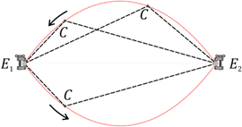
Figure 1. Helmholtz motion in an idealised bowed string with fixed ends E1 and E2. The dotted curve is the trajectory followed by the string's corner: the succession of two parabolic arcs. Arrows mark the direction of motion of this corner.
Download figure:
Standard image High-resolution imageThis type of movement occurs only for an idealised, one-dimensional string without friction. Clearly, the friction between the moving bow and the vibrating string must transfer enough power to the string to overcome the losses from internal dissipation, viscous drag from the air, and loss via the non-rigid end supports [13–15]. However, in the ideal case, once started, a movement of this type will continue indefinitely in a string with fixed ends. This property is essential for the derivation of the shape of the envelope of the Helmholtz motion based on energy conservation criteria in the final section of this article.
Needless to say, this movement in a violin string surprises colleagues who are not aware of this effect, and if it were not for the fact that it can be experimentally shown [8, 16, 17], they would find it hard to believe that such a movement is possible, let alone accept that the movement was observed by the German physicist/physician Hermann von Helmholtz in the second half of the 19th century using a vibration microscope [11].
Taking into account that the corner C covers a distance that is twice as long as the string in the time corresponding to its vibration period (that is, the duration of the note), in the case of the E string, for example, the speed of the corner is about 430 m s−1. This can be easily obtained from the fundamental frequency of the E string, 659.3 MHz, which gives a period of 1/659.3 = 1.517 × 10⁻³ s for a complete turn of the corner. The velocity of the corner is given by the distance travelled by the corner in one period (twice the length of the string) divided by the period. For a standard violin string of length 0.325 m, this gives 0.65 m 1.517 × 10⁻³ s = 428 m s−1. If we compare the speed of the corner to the speed of the propagation of sound through air, which is approximately 340 m s−1, we can see that this is a considerable speed, and the movement is not easily observed with the naked eye. The observations of Helmholtz therefore have great merit.
The main objective of this work is to construct a detailed kinematic theory of this simple Helmholtz motion in a bowed string without the use of ordinary Fourier analysis. The pioneering work by Helmholtz [11] and Donkin [12] was carried out by means of Fourier analysis, whereas Raman's (1918, section IV) approach was graphical [18], starting from the velocity profile of the string, rather than from the deflections, as we do here (moreover, Raman does not provide a demonstration of the parabolic shape of the movement in his 1918 monograph, although he does in a previous paper, in this case using a Fourier approach similar to that of Helmholtz and Donkin) [19]. Most of the work done since these three pioneering studies has been dedicated to the dynamics of the bow-string system, and to how the Helmholtz motion can be sustained in a real violin by including in the analysis friction forces, applied pressures, energy losses and other complicating issues [20–24]. The shape of the curve tracked by the Helmholtz corner has not been a matter of attention since then, and we aim to revisit this interesting problem here from a different point of view. Obviously, in our analysis of the simple Helmholtz motion we are in the domain of small deformations.
First and foremost, we verify that the function  the transverse displacement of each point x of the string at any instant t during the simple Helmholtz motion, is a solution of the wave equation by writing it as the addition of two waves travelling to the right,
  and to the left,
  Finding these two waves is probably not a problem that a student would like to see in a university exam! However, one must be certain that since
  is a possible actual motion, it must be a solution of the equation of motion, and that the equation of motion is the wave equation. Since
  does not have a sinusoidal profile, the verification of this as a solution of the wave equation is highly instructive, and even more so if we avoid the well-trodden path of Fourier analysis.
Our proposal consists of the following aspects. In section 3, we show that the function  corresponding to simple Helmholtz motion is a solution of the wave equation in one dimension. Since
  is the position of the corner C at any instant t, we show in the same section that the envelope of the trajectory described by this corner, that is to say
  is the succession of two parabolic arcs. In section 4, we analyse the velocities corresponding to simple Helmholtz motion, and show that
  the transverse speed of each point of the string at any instant, is also a solution of the wave equation. Finally, in section 5, we calculate the total kinetic energy of the string, its elastic potential energy and their sum, the total energy E, and its scaling relation to
  From the conservation of total energy, we are again able to deduce the shape of the trajectory of the corner.
3. The Helmholtz motion as a solution to the wave equation
The one-dimensional form of the wave equation is given by

where c is the velocity of propagation of any wave in the string, which is well known to be related to T, the string tension, and μ, the string mass per unit length, through

In equation (1),  represents the transverse displacement at any time of any point x on the stretched string of length l, that is to say, for
  The boundary conditions
  correspond to fixed ends, as indicated in all the figures in this paper by
  and
and 
To show that the simple Helmholtz motion  depicted in figure 1 is a solution to the wave equation (1), we will prove that this function can be constructed as the sum of two waves, one travelling to the right,
  and the other to the left,
  This means that
  can be written as

with

and

where K is a constant that, as we will show later, depends only on the total energy E of the string. The family of equations represented in equations (4) and (5) give the values of f and g for any x (−∞ < x < ∞) at any time t > 0. For instance, for n = 0 and t = 0, the interval of x values for which equations (4) and (5) are defined is −l ≤ x ≤ l:

The shape of the f and g profiles is a parabola, as represented in figure 2 for  Note that the repetition of this basic shape, displaced by a distance of
  (that is, twice the length of the string), generates the periodic functions f and g. The displacement of the basic parabola centred at x = 0 (for t = 0) is accomplished by changing the value of n in equations (4) and (5): negative n-values displace the parabola to the left and positive n-values to the right. The end result is a continuous piecewise function which is differentiable at all points except where two consecutive copies of the basic parabola join: this non-differentiability at specific points is the underlying reason for the apparition of the corner in the Helmholtz motion. We can see from figure 2 that at
  if the f and g waves are added, the transverse displacement is such that
  for all x: the string is, therefore, in a horizontal position. It is important to stress here that the parabolas shown in figure 1 and those shown in figure 2 are not the same; those in figure 1 depict the trajectory of the corner of the string during the Helmholtz motion, whereas those in figure 2 depict the wave functions that should be added to give the shape of the whole string (including the corner, of course) at any instant t > 0. Obviously, both sets of parabolas are related. The period of the corner depends on the frequency of the note played (for example, the period of the corner for the E string is 1.517 × 10⁻³ s, as already shown above), whereas the period of the parabolic f and g waves is 2l/c (see equations (4) and (5)), where c, the propagation speed of the wave, depends on the string's tension and mass, properties that also influence the fundamental frequency of the note.
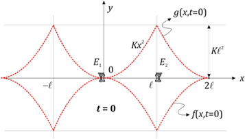
Figure 2. Shape and location of the right-travelling function f and the left-travelling function g, whose addition gives the Helmholtz motion, at t = 0. The figure shows the complete parabolas for the case n = 0 (up and down parabolas centred at x = 0, and half the parabolas for n = ±1), displaced a distance 2l on the x-axis.
Download figure:
Standard image High-resolution imageIn order to prove that the addition of these two parabolic profiles propagating in opposite directions gives the Helmholtz solution outlined in figure 1, we must obtain triangular profiles in their superposition at almost any instant (except for those instants in which the string is horizontal, when the corner is at either of the two fixed ends of the string). To demonstrate that the resulting profile is indeed triangular, figure 3 shows the f and g waves at some arbitrary time t between  (the instant at which the string is in a horizontal position and the corner is at the right-hand end E2 of the string) and
  half the period (the instant at which the string is again in a horizontal position but the corner is at
  the left-hand fixed end of the string). The g-wave has moved to the left a distance equal to
  while the f-wave has moved to the right the same distance
  This is shown in figure 3, where we take as an example
  with
with 

Figure 3. Shape and location of the f and g functions at an instant t corresponding to x0 = 2l/3. The f function has moved to the right a distance ct and the g function the same distance to the left.
Download figure:
Standard image High-resolution imageNow, to add the f and g profiles, we divide the string into two parts:
- (a)
- (b)For
 i.e. to the right of the position of the corner, we again have a linear transverse displacement given by another straight line,


as indicated in figure 4. In equation (8), the first bracketed term of the right-hand expression includes a 2l term; as figure 3 shows, this can be written as ![$K{[(l-ct)+(l-x)]}^{2}.$](https://content.cld.iop.org/journals/0143-0807/40/1/015802/revision2/ejpaae8b5ieqn36.gif)
We now obtain the envelope of the corner position by calculating its transverse displacement,  at any instant:

where its maximum value for  i.e.
i.e.  is given by

If we define the variable  as shown in figure 4, where
  is the abscissa of the corner taken from the middle point of the string, we can rewrite equation (9) as

with  Thus, we can deduce from this equation that the trajectory of the corner, the dashed line in figure 4, from
  to
to  (i.e. when
  ) is a parabola. Naturally, we can say the same for the other semi-period, in which the parabola is upside down.
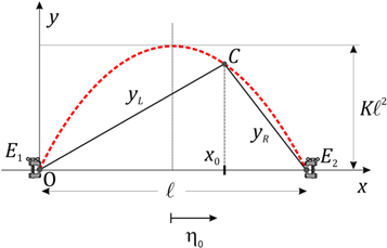
Figure 4. Shape of the string at an instant corresponding to x0 = 2l/3 (black line with corner at C) composed of the two linear sections yL and yR. The trajectory of the corner is marked by a dashed line. The new variable η0 = l/2—ct translates the origin of the coordinates to the middle point of the string (l/2).
Download figure:
Standard image High-resolution imageAs already noted, both parabolas, the trajectory of the corner and the parabolic profiles of f and g, are not the same. The semilatus rectum in the former parabola is, according to equation (11), four times greater than the corresponding to the f and g profiles.
Emphasis should be placed on the necessary condition of the smallness of the transverse oscillations, and thus on the validity of equation (1). From equation (10) it follows that the condition  must be fulfilled, or

where  is a dimensionless magnitude.
4. The velocity of the string as a sum of waves

As a consequence of the simple Helmholtz motion being a solution of the wave equation, equation (1) with  written as in equation (3), it follows that the velocity of each point of the string is given by

where 
 and the prime indicates derivatives with respect to u or z. We therefore have another function which is a superposition of waves:

where  and
and  are
are  and
and  respectively, and since f and g have parabolic profiles, their derivatives are straight lines. From figure 2, we therefore obtain

These two profiles, which are periodic functions of period  are represented in figure 5 for
  the time at which both functions are superposed. At any other time t,
  the n-wave has moved to the left a distance equal to
  while the p-wave has moved to the right the same distance
  as shown in figure 6. According to equation (14), the velocity at each point is the sum of both waves, the boundary conditions of zero velocity at the ends being guaranteed at any instant. Note in the same figure that for
  the string velocity is upwards, while for
  it is downwards; there is also a discontinuity in the velocity at
  the abscissa of the corner, and thus an infinite acceleration in the corresponding element of the string [25].
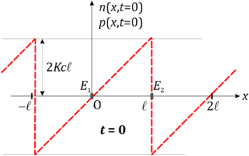
Figure 5. Velocity profiles p(u) and n(z) at t = 0.
Download figure:
Standard image High-resolution image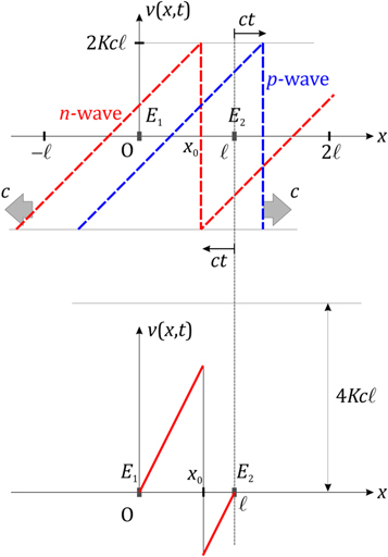
Figure 6. Shape and location of the n and p functions at the instant t, corresponding to x0 = 2l/3. The p-function has moved to the right a distance ct, and the n-function has moved to the left the same distance.
Download figure:
Standard image High-resolution imageFrom this graphical superposition it can be deduced that at  when
when  the velocity of each element of the string is positive, with the maximum possible value (at
  ) equal to
  At
At  one half of the oscillation period,
  and the corner is at
  At this instant, the velocity of each element of the string is negative, and the minimum velocity value is
  Both
Both  and
and  give horizontal positions for the string and are the instants at which the kinetic energy is maximum. The kinetic energy at these positions is the constant total energy E of the string, since there its potential energy is taken as zero.
As for the acceleration of the string, we can observe that for most of each period, any given element moves at constant velocity. There is no net force acting on it because for most of the time the form of the string is the same straight line on both sides of the element. Thus, any given element moves at constant velocity at all instants within a period, except for the two instants in which the element is reached by the corner; at these instants,  becomes
  This effect can be seen qualitatively in figure 4, where the shape of the string is depicted at a particular instant. Here, the left-hand string segment is moving downwards as the corner moves from left to right, while the right-hand string segment is moving upwards. Each material point on the string has a speed that is proportional to the distance to the fixed end (where the speed is zero), and which is negative in the left-hand segment and positive in the right-hand segment. Thus, the maximum speed corresponds to the material points flanking the corner, upwards to the left of the corner and downwards to the right, with a discontinuity at the corner where the acceleration, as a consequence, is infinite. Although it may sound odd to refer to an 'infinite acceleration', we are dealing with the solution of the wave equation, and must accept all its consequences. Remember that in this paper we are concerned only with the simple Helmholtz motion, where energy losses are zero. In a real violin string, friction and other losses tend to smooth the corner, which is no longer sharp but a bend with very small curvature, giving rise to large (but finite) accelerations.
Note that the velocity of each point on the string could also be obtained directly from equations (7) and (8), and so
in accordance with figure 6.
5. Using energy conservation to obtain the trajectory of the corner
5.1. The elastic potential energy
For the abscissa  of the corner, the elastic potential energy of the stretched string is a function of
  the transverse displacement of the corner, and can be calculated as the work done by the external force
  necessary to deform the string quasi-statically, starting from its horizontal equilibrium position.
To calculate this  with Cartesian components F and H, as a function of any intermediate position
 figure 7 shows all the forces acting on a string element of a particular mass located just at the corner, assuming the same string tension on both sides of the element. Since we are dealing with small transverse displacements, both horizontal components of the string forces acting on the element are almost the same, and so we consider H to be negligible in comparison with F. Now if the mass of the element tends to zero, the sum of forces acting on the element must do the same in order to prevent the acceleration of the element becoming infinite. Thus, according to figure 7, writing
  where
where  is a unitary vector in the upward direction as shown in the figure, we have

which can also be written as

Figure 7. Forces acting on the corner to deform the string quasi-statically.
Download figure:
Standard image High-resolution image
For a given value of the total energy E, the potential energy of the string is given by

and so, by substitution of equation (17) into equation (18),
These integrals are straightforward, and we can therefore easily obtain

As we are considering small deformations of the string, we take

and we finally obtain

where  is directly proportional to the total energy E of the string, as will be shown in equation (27).
5.2. The kinetic energy
To calculate the kinetic energy of the string, we consider, for instance, the second velocity diagram of figure 6. We can write
where μ is the mass of the string per unit length. As shown above, the kinetic energy is a maximum for  and we can differentiate equation (22) to obtain the value of
  for the minimum kinetic energy. We obtain
and so, finally, we obtain the relation between K and the total energy E of the string, which is given by

From here,

where  is the total string mass, and using the condition in equation (12), we obtain from equation (24) that for small displacements

5.3. The total energy
Since there are no losses of energy in our idealised Helmholtz motion, we can express the energy conservation as
and, by substituting equations (21), (22) and (24) with  we obtain
By setting  we obtain for
and by substitution of  from equation (24),

where the plus sign is valid for  i.e. from
  to
to  After the substitution of equation (27) into equation (21), we can immediately see that the maximum value of the potential energy is reached when x0 = l/2 (i.e. when the corner is midway between the fixed ends), and the minimum value when x0 = 0, l (i.e. when the corner is at either the left-hand or right-hand ends, and the string is horizontal everywhere). When the potential energy is a maximum, half of the string is moving upwards with a velocity proportional to the distance to the fixed end, and the other half is moving downwards with the same velocity profile. Conversely, when the potential energy is a minimum, the complete string is moving either upwards (when the corner is at the left-hand fixed end) or downwards (when the corner is on the right-hand fixed end).
Now, with a change of variable for the corner position  where
where  is the abscissa of the corner taken from the middle point of the string, we obtain from equation (27)

with

in accordance with equation (11). We therefore again obtain the result that the trajectory of the corner is a parabola. Note the relation 
6. Conclusion
We have shown in this paper that it is worthwhile to prove that the simple Helmholtz motion is, against all odds, a solution of the wave equation. A discussion such as this provides numerous opportunities for the teacher to 'spiral back' and more effectively help students to understand the way that solutions to the wave equation work, keeping in mind the superposition principle.
A further benefit that should not go unmentioned is the introduction and calculus of E, the total energy of the string, which, as can be expected, completely characterises the two waves f and g, the components of the simple Helmholtz motion, through the value of K(E) given in equation (25).
Finally, we can justify the title of the paper, 'Parabolic curves in a Helmholtz solution for a bowed string', since f and g have a parabolic profile and the envelope of the position of the corner also has a different parabolic form.
Footnotes
- 1
We can read in [6] 'One way to study the spectrum and the modes is by thwacking the bridge with a small hammer and measuring the violin's output and motion. Around 280 hertz lies the A0 mode, in which air flows in and out of the f-holes on the violin's belly'. This is the vibration frequency of a violin considered as a Helmholtz resonator.