
Abstract
Non-thermal plasma is a key component in gas lasers, microelectronics, medical applications, waste gas cleaners, ozone generators, plasma igniters, flame holders, flow control in high-speed aerodynamics and others. A specific feature of non-thermal plasma is its high sensitivity to variations in governing parameters (gas composition, pressure, pulse duration, E/N parameter). This sensitivity is due to complex deformations of the electron energy distribution function (EEDF) shape induced by variations in electric field strength, electron and ion number densities and gas excitation degree. Particular attention in this article is paid to mechanisms of instabilities based on non-linearity of plasma properties for specific conditions: gas composition, steady-state and decaying plasma produced by the electron beam, or by an electric current pulse. The following effects are analyzed: the negative differential electron conductivity; the absolute negative electron mobility; the stepwise changes of plasma properties induced by the EEDF bi-stability; thermo-current instability and the constriction of the glow discharge column in rare gases. Some of these effects were observed experimentally and some of them were theoretically predicted and still wait for experimental confirmation.
Export citation and abstract BibTeX RIS
1. Introduction
Non-thermal plasma technologies continuously expand into various fields of human activity. Non-thermal plasma is used for cleaning waste gases, modification of polymer surfaces, sterilization of medical instruments, treatment of living cells, excitation of gas lasers, ozone generation, plasma-assisted ignition, flame holding, surface etching, plasma-assisted chemical vapor deposition, and others [1]. Plasma properties can be varied widely by changing discharge type, gas composition and pressure, plasma configuration and mode of discharge operation. Mathematical modeling of processes in a bulk of plasma plays an important role in development of plasma technologies. Theoretical modeling can significantly help in finding optimal conditions for a given plasma technology. A specific feature of non-thermal plasma is the strong variability of its properties with changing experimental conditions (gas composition, pressure, pulse duration, E/N parameter, E is the electric field strength, N is the gas number density). Reactivity of plasma, its key property for most applications, is associated with a high average electron energy, which is controlled by electric field heating and inelastic collision losses. Typical electron energy distribution function (EEDF) is far from the Maxwellian and must be calculated numerically for specified conditions. In contrast to the thermal plasma, the EEDF shape in any non-thermal plasma cannot be characterized by a single parameter (such as the average electron energy).
Moreover, variations of the EEDF shape induced by changes in plasma density or the electric field may cause instabilities in plasma resulting in various non-uniform patterns in discharges. Here we provide an overview of research activity in this particular field. This article is devoted to studies of phenomena resulting from non-equilibrium and non-linear behavior of the EEDF. The effects under consideration are the following:
- negative differential electron conductivity (NDC),
- absolute negative electron mobility,
- EEDF bi-stability,
- thermal-current instability,
- constriction of the plasma channel in rare gases,
- striations.
2. Basic expressions
Electrons are much lighter than atoms, ions and molecules. Therefore, the direction of electron velocity randomizes for a few elastic collisions with heavy particles. Then the electron velocity distribution function after a few elastic collisions can be approximated by a sum of two terms: a spherically symmetric function, f0 (r, v, t), and a first spherical harmonic, f1 (r, v, t):

Here f1 is a vector function, v = |v|, r and v are vectors of electron location and velocity, respectively.
When the spatial scale for variations of plasma parameters, L, is much greater than the electron free path length, λm, and the characteristic frequency of parameters variation, 1/τ, is much smaller than momentum-transfer frequency vm, (λm ≪ L, 1/τ ≪ vm), f1 can be expressed in the following form:

qm(u) is the total momentum-transfer cross section as a function of electron energy u, ne is electron number density, N is the gas number density, E is the electric field strength vector, e is the electron charge. In this approximation, the spherically symmetric function (EEDF) satisfies the Boltzmann equation (BE):
where m is the electron mass, E is the electric field strength module. The second term in the left-hand side of (3) reflects the spatial diffusion and the drift of electrons; the third describes the interaction of the electric field with the electron diffusion flux; the fourth is the electron heating by electric field, the last is the collision integral describing energy exchange in electron–electron and electron–heavy particles collisions. The distribution function f0 is normalized as follows:

Equation (3) gives an idea about the main processes participating in the formation of the EEDF, but it is very complicated for doing practical calculations.
In the limit of (λu/L) ≪ 1 and (νu τ) ≫ 1 (here νu is the electron energy relaxation frequency and λu is the energy spatial relaxation length), the steady state and spatially uniform EEDF satisfy the equation

The term St(nef0) is equal on the order of magnitude to νunef0.
Various electron scattering processes can be easily taken into consideration in BE: elastic scattering of electrons from atoms and molecules (taking into account the finite gas temperature), excitation of their electronic and vibrational states by electron impact, second kind (super-elastic) electron collisions with excited atoms and molecules, ionization by electron impact, Coulomb collisions and others. Forms of the specific terms in the collision integral can be found, for example, in [2]. The numerical solution of BE is a regular method for the EEDF and electron kinetic and transport coefficients' calculations.
Another approach is the direct simulation of the electron motion in the gas using the Monte Carlo (MC) technique (see, for example, [3–7]). The main features of this approach are the following: the free path of an electron along the trajectory (or time interval between collisions) is assigned randomly with a proper probability density. The trajectory of an electron and its energy between collisions are calculated by integration of the equation of motion. The type of collision process occurring after a free flight is assigned randomly, and the probability of each process is taken proportionally to its cross section (weighted with the partial concentration of the respective mixture component). The direction of motion after a collision is assigned randomly as well. A large number of test electrons are launched, and the EEDF and electron kinetic and transport coefficients at a given position (or moment of time) are calculated using proper averaging procedures. As a rule, in MC simulations the motion of heavy particles is ignored. Inclusion of Coulomb collisions in MC approaches represents a significant challenge (see comments and references in [8]), and in conventional MC studies these processes are not taken into consideration.
Direct integration of (3) results in a well-known electron continuity equation:

Qe combines the terms including ionization, attachment and recombination processes leading to variations of the electron number density. Numerical evaluation of Qe requires knowledge of cross sections for all processes included in a model. The transverse diffusion coefficient, D⊥, and the drift velocity, W, are expressed in the form
Electron continuity equation (6) in combination with ion continuity equations and a system of balance equations for chemical species in ground and excited states form a fluid model in local-field approximation. In this connection, rate coefficients for electron-induced processes are to be found from the solution to equation (5) with a local value of the electric field strength, E. Generally, the value of E varies in space and time. Its variation can be found from electro-dynamic equations and parameters of an electric circuit.
While implementing the fluid model, one has to be careful about limitations on its applicability. General strong inequalities (λu/L) ≪ 1 and (νut) ≫ 1 may not ensure accuracy of the results of numerical calculations. The point is a strong dependence of rate coefficient magnitudes on the EEDF shape for inelastic processes with a high-energy threshold (ionization, dissociation, excitation of electronic states). The electron energy spatial relaxation length, λu, and temporal relaxation frequency, νu, both relate to a body of the EEDF. Actually, the relaxation of the high-energy tail of the EEDF is frequently much slower. The spatial relaxation length of the EEDF tail is longer than λu. It was shown in [9] that permissible spatial gradients (1/L) of the EEDF high-energy tail in the non-uniform electric field are limited by a condition:
 is the electron mean energy,
 . Similar inequality limits permissible temporal rate of plasma parameter changes [10].
The energy exchange in e–e collisions is very fast, and its rate can be characterized by the effective cross section of the order of 10−12 cm2 at the energy equal to l eV. The e–e collisions exert an influence on the shape of the EEDF. The contribution from e–e collisions becomes comparable to that of electron–atom collisions when the degree of ionization α = ne/N is about 10−7. At high electric field or large electron number density, efficient excitation of heavy particles by electron impact can strongly increase the number of excited atoms and molecules. Then, electron collisions with excited atoms and molecules resulting in stepwise excitation (dissociation/ionization) and quenching of the excited particles should be taken into account [11]. As was noted in [12], the electron–ion (e–i) collisions in Ar plasma can also play an important role. To take into account (e–i) collisions one has to add in total momentum-transfer cross section qm(u) the term reflecting (e–i) collisions qei(u):

here Ni is the ion number density and qea(u) is the momentum-transfer cross section for the electron scattering from neutral particles.
3. Negative differential electron conductivity
An effect of the electron drift velocity decreasing with growing electric field is traditionally named as the negative differential conductivity (NDC). Mixtures of gases, in which the NDC occurs, are potential candidates for using in electron-beam-sustained discharge (EBSD) switches [13–15] and in gas-filled detectors for radiation detection and dosimetry [16–17].
The electric resistance of plasma in a conventional diffuse discharge switch grows as a function of the electric field due to increase in the electron attachment rate. Fall down of the drift velocity with E/N accelerates growth of the plasma resistance and increases its magnitude. As a result, the voltage supplied is redistributed between the switch and the load faster and more effectively. Extensive experimental data on the drift velocity in gas mixtures CH4–Ar, CF4–Ar, and mixtures C2F6, C3F8, CF3OCF3 with Ar or CH4 are given in [14].
The most commonly used gas mixture in radiation detectors filling gas is (CH4 : Ar = 1 : 9) mixture (P-10). The authors of [18] performed studies on various gas mixtures, which have higher than in (P-10) mixture drift velocity with its minor variation in a wide range of E/N values. For such mixtures gas-filled detectors for a convenient E/N range have a faster response as compared with the standard (P-10) mixture. It was found that the best characteristics have the ternary mixture CF4 : C2H2 : Ar = 1 : 1 : 8.
The NDC under swarm conditions is rather sensitive to shapes of electron scattering cross sections. That is why the swarm data on the electron drift velocity in gaseous mixtures exhibiting the NDC were used to normalize electron scattering cross sections for vibrational excitation of molecules: CO [19], N2 [20–21] and CO2 [22].
The NDC manifests itself in an EBSD in a form of spontaneous discharge voltage/current oscillations being a direct analog of Gunn microwave generator in semiconductors [23]. The oscillations induced by the NDC were observed experimentally in the EBSD by a number of authors (see [24–26]). This phenomenon was found to limit operation ranges for gas lasers [27] and generators of singlet delta oxygen molecules [28].
The first observation about the electric current oscillations induced by the NDC was made in the work of [24] for the EBSD in Ar mixed with (2–5)% N2 or CO additives. At a certain level of voltage applied to the discharge gap, the luminescent layers moving from the cathode to the anode were formed, while in the discharge circuit the oscillations of the discharge current were detected. The propagation velocity of the layer is nearly equal to the electron drift velocity, W, and the period of the oscillations of the discharge current is Tosc ∼ d/W, where d is the distance between the electrodes.
Later, similar studies have been performed for (0.1–1)% HCl–Ar mixtures [25] in the EBSD at atmospheric pressure. The electric current oscillations were detected, and W(E/N) was calculated theoretically. A typical waveform of the discharge current in the event of the instability is shown in figure 1. Oscillations have a period of (0.5–1) µs at the inter-electrode spacing of 1 cm. The NDC phenomenon has got much attention and was observed in many experiments. Discussion in this section is organized as follows: section 3.1 discusses the data on molecular species and gas mixtures possessing Ramsauer–Townsend (R–T) minimum in qm as a function of the electron energy; section 3.2 discusses studies on effects associated with e–e, e–i and second-kind collisions for pure rare atomic gases and their binary mixtures.
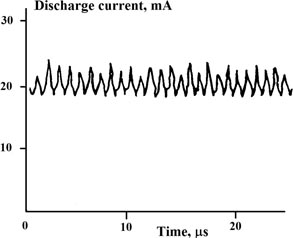
Figure 1. Oscillogram of the discharge current, 1% HCl–Ar [25].
Download figure:
Standard image High-resolution image3.1. Pure molecular gases and their mixtures with rare gases
The NDC was observed for a number of molecules: CH4 [29–31]; C2H4 [32]; CF4 [33–34]. The perfluoroalkanes C2F6 and C3F8 exhibit the pronounced NDC similar to but smaller in magnitude than that in CH4 [34]. The electron drift velocities in BF3 and SiF4 demonstrate the NDC in some ranges of the electric field strength similar to but smaller in magnitude than those in CH4 and CF4 [35]. The momentum-transfer cross sections for selected atoms and molecules possessing the R–T minimum are shown in figure 2. Figure 3 shows the experimentally measured W(E/N) in pure molecular gases (CF4, CH4, C2H4) in comparison with the results of numerical solutions of the BE at room gas temperature.
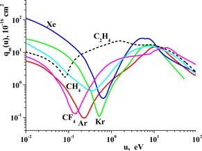
Figure 2. Momentum-transfer cross section versus electron energy for Ar, Kr, Xe [36], CH4 [37], C2H4 [38] and CF4 [33].
Download figure:
Standard image High-resolution image
Figure 3. Electron drift velocities versus E/N. Solid lines are the results of calculations: CF4 [39]; CH4 [40]; C2H4—present work (cross sections are from [38]). Markers are the experimental data: •—[33]; ▴—[31]; ▾—[30]; ▪—[32].
Download figure:
Standard image High-resolution imageThe authors of [41–43] have analyzed what special features in the electron collision cross sections are responsible for the NDC appearance. The NDC can occur when an increase in the E/N parameter leads to an abnormally large increase in vm value. Then, the enhanced randomization of directions of the velocity vectors can decrease the drift velocity even though the mean electron energy increases. The combination of the rapidly increasing elastic cross section or Ar, Kr and Xe above the R–T minimum and the vibrational excitation cross section for some molecules is known to produce the NDC in molecular–rare-gas mixtures at a small fraction of the molecular gas [44–45, 19, 14, 46]. The R–T minimum is most deep for the transport cross section of Ar (see figure 2). Therefore, the appearance of NDC in mixtures of molecular gases with Ar is more probable.
Figure 4(a) shows W(E/N) for mixtures CO–Ar of variable composition calculated in this work, including limits of pure CO and Ar gases. It is seen that the NDC occurs within certain ranges of CO concentrations and of E/N values. Theoretical curves for CO fractions 1%, 2%, and 5% are compared with the swarm data [19] for these mixtures. Good agreement between calculated and measured data proves that the self-consistent set of cross sections for CO is rather accurate. The regions, where the NDC effect is predicted for Y–Ar mixtures (Y denotes CO, N2 or O2), are shown in figure 4(b) along with available experimental data. Results presented in figure 4(b) are calculated by taking into account loss and gain of the electron energy in the elastic scattering from atoms and molecules, excitation and de-excitation of rotational states, excitation of vibrational and electronic states and ionization by electron impact. Electron scattering cross section sets were taken from [49] for N2, CO and from [50] for O2. Vibrational excitation of molecules was assumed to be low, and electron collisions with vibrational-excited molecules were neglected. The concentrations of molecular additives, below which the NDC disappeared, and corresponding E/N values (figure 4) are as follows: 66 ppm N2 at E/N = 1.1 Td; 66 ppm CO at E/N = 0.65 Td; 400 ppm O2 at E/N = 0.054 Td.
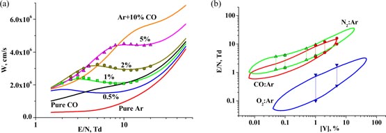
Figure 4. (a) Electron drift velocity versus E/N for CO–Ar mixtures, markers are the experimental data [19], lines are the results of calculations, T = 300 K; (b) regions of the NDC effect in Y–Ar mixtures on the E/N–[Y] plane, [Y] is the percentage of Y component (N2, O2 or CO). Closed lines show predicted regions of the NDC, and markers are the experimental data: ▴ (N2)—[47]; ▪ (N2)—[20]; • (CO)—[19]; ▾ (O2)—[48].
Download figure:
Standard image High-resolution imageIn fact, electrons in non-thermal plasma effectively excite vibrational and electronic states of molecules. The stepwise and second-kind collisions can remarkably change the EEDF shape [11]. In [51] it was shown numerically that growth of vibrational temperature of N2 molecules leads to the disappearance of the NDC effect in the mixture of N2 : Ar = 1 : 99. A similar effect takes place in gas mixtures CO : Ar. A specific feature of molecular vibration kinetics for N2 and CO is the strong difference in vibrational relaxation and vibration–vibration exchange rates. The latter is much faster. As a result, at a moderate vibration excitation rate and low gas temperature vibrational distribution function (VDF) in N2 and CO strongly deviates from the Boltzmann distribution. The VDF under these conditions has a long plateau at intermediate vibrational levels. The analytical theory [52] for this case provides an approximate expression for the VDF. In the theory, a parameter TV defined by formula n(v = 1)/n(v = 0) = exp(−E1/kTV) serves to characterize the strongly non-equilibrium VDF (E1 is the vibration quantum energy, v is the number of vibration level). Within the frame of this theory, we have made numerical calculations by taking into account electron energy exchange with vibrational excited molecules. Figure 5(a) shows how the W(E/N) curve for CO : Ar = 2 : 98 mixture transforms with the growth of an effective vibrational temperature, TV, at the fixed translational gas temperature equal to 300 K.
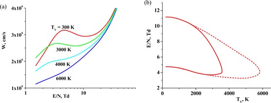
Figure 5. (a) W(E/N) and (b) the region with the NDC on the E/N–Tv plane calculated for the CO–Ar = 2 : 98 mixture and T = 300 K. Solid lines are for the non-equilibrium VDF [52]. Dashed line is for Boltzmann distribution over vibrational levels.
Download figure:
Standard image High-resolution imageFigure 5(b) shows the regions on the (E/N–TV) plane for mixture CO : Ar = 2 : 98 where the NDC is predicted. It is instructive to compare the results found for non-equilibrium (solid line) and equilibrium (dashed line) VDFs. It is seen that the vibrational non-equilibrium causes the region to diminish with the NDC.
With an increase in the ionization degree, α = ne/N, Coulomb collisions can influence the EEDF shape and, accordingly, the NDC appearance. Figure 6 illustrates the influence of e–e and e–i collisions on the NDC region on the (E/N–α) plane (solid-line boundary) for a mixture N2 : Ar = 2 : 98 at Tv = T = 300 K. It is seen that at α ⩾ 3 × 10⁻⁴ the NDC disappeared. To distinguish between effects produced by e–e and e–i collisions, calculations were performed neglecting e–i collisions (dashed line). In this case, the NDC is predicted to exist even at α > 0.1. This indicates the importance of the e–i collision input into qm amplitude [12].
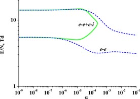
Figure 6. E/N values at the boundaries of NDC appearance as a function of α = ne/N calculated for N2 : Ar = 2 : 98 mixture at Tv = T = 300 K. The solid line is for the case when both e–e and e–i collisions are taken into account. The dashed line is for the case when e–i collisions are neglected.
Download figure:
Standard image High-resolution imageIt was revealed in swarm experiments [22] that in the CO2–Ar mixtures, at certain concentrations of CO2, two separate NDC regions may appear. Figure 7 (curve 1) shows two regions, in which measured W(E/N) decreases as a function of E/N in Ar with 0.203% of CO2 admixture. Results of these measurements along with swarm data for pure CO2 were used in [22] to correct both the vibrational excitation and transport cross sections in CO2, as well as the cross sections for excitation of CO2 electronic states. The set of cross sections proposed in [22] is, obviously, the most reliable at the present time.

Figure 7. W versus E/N. Line 1 and markers are results from [22], gas mixture is 0.203% CO2 in Ar, line 2 is calculated for Tv = 300 K, and line 3 is calculated for Tv = 1500 K, gas mixture CO2 : Ar = 1 : 9 [53].
Download figure:
Standard image High-resolution imageOur BE calculations of swarm data with variation of shapes of vibrational excitation cross sections allow us to associate the appearance of two humps in the W(E/N) with a relatively slow decrease in the excitation cross section for the CO2 (0 0 1) mode at the high-energy side [53]. This finding is confirmed by the fact that in H2O–Ar mixtures the double-humped shape of the W(E/N) disappeared. The faster decrease in the vibrational excitation cross sections at higher electron energies is a cause of its disappearance [53].
It was shown in [53] that the increase in CO2 concentration from 0.203% to 10% results in noticeable growth of the electron drift velocity at E/N > 0.1 Td (compare curves 1 and 2 in figure 7). Note that the double-humped shape of the W(E/N) curve remains but the amplitude of wavy structure diminishes. Numerical calculations [53], by taking into account the second-kind electron collisions with vibrationally excited CO2 molecules, have shown that in the CO2–Ar mixtures the degree of vibrational excitation negligibly affects the double-humped shape of the drift velocity (figure 7, lines 2 and 3). In the calculations, the temperatures of all vibrational modes of the CO2 molecule were assumed to be equal to the gas temperature, Tv = T.
For Kr and Xe, the R–T minimum is located at higher energies (figure 2) in comparison with Ar. This feature explains why the predicted double-humped shape of the W(E/N) is less pronounced in CO2–Kr mixtures and disappears in the CO2–Xe mixtures [53]. It was shown theoretically that the double-humped shape of W is most impressive in 10% CO2–Ar and 15% CO2–Kr mixtures. Thus, among binary mixtures of rare–molecular gases the double-humped curve of W(E/N) was found only for the CO2–Ar (Kr) mixtures.
A three-component mixture of two molecular gases and a heavy inert gas provides more variety in behavior of energy loss rate as a function of electron energy and better chances to realize double-humped behavior of W(E/N). As an example, the double-humped shape of the W(E/N) curve predicted theoretically [53] for the CH4–H2–Ar mixture is shown in (figure 8). In these mixtures, the drift velocity changes not so much in a wide range of E/N from 0.2 to 10 Td.

Figure 8. The electron drift velocity W(E/N) in the CH4–H2–Ar mixture (1% H2) at various concentrations of CH4: (1) 2% CH4, (2) 1% CH4 and (3) 0.5% CH4 [53]. Tv = 300 K.
Download figure:
Standard image High-resolution imageThe difference in W(E/N) values for the two NDC regions calculated [53] was found to be quite large in the H2O–N2–Ar and SF6–N2–Ar mixtures. The drift velocities differ by a factor of 2–3. Since the high-field layers propagate with the velocity nearly equal to the electron drift velocity, the appearance of oscillations in two NDC regions can be easily detected experimentally due to a notable difference in oscillation frequencies. Verification of these theoretical predictions can be easily carried out by respective experiments with an EBSD in gas mixtures predicted.
The double-humped shape of the W(E/N) curve is a rather fine effect, which requires specific shapes of both the transport cross section for electron scattering from inert gas atoms and cross sections for inelastic scattering from molecules. For binary mixtures, this effect is found only in the CO2–Ar (Kr) mixtures.
For ternary mixtures, the required energy dependence of inelastic processes rates can be realized by changing the concentrations of the molecular components.
3.2. Rare gases
The NDC can take place also in mixtures of Xe with He [54–55]. The elastic collisions with He atoms are accompanied by energy exchange, which plays a role similar to inelastic collisions in molecular gas–rare gas mixtures. Results of measured swarm data on W(E/N) for a variety of He concentrations in the mixtures He–Xe [56] are in qualitative agreement with that predicted by [54].
The use of external ionization, such as a fast electron beam or an x-ray source, allows one to control the ionization degree and E/N, independently. If an EBSD is implemented for pumping gas lasers or in plasma-chemical reactors, the excitation degree is not negligible and can exert an influence on electron transport in rare gas mixtures. It means that the values of ionization degree (α) and of electronic excitation degree δ = N*/N(N* is the number density of excited atoms) are correlated and both have an influence on the EEDF shape and electron transport coefficients. To get a deeper insight into the mechanisms of NDC formation, it is convenient to analyze roles of these parameters as independent ones. The authors of [57] have carried out detailed numerical studies on the NDC in He–Xe mixtures. It should be emphasized that the set of electron scattering cross sections used in [57] enable an accurate reproduction of swarm data [56]. The influence of He percentage, α and δ on the NDC was analyzed. Figure 9 demonstrates that at low He percentage Coulomb collisions extend the E/N range with the NDC at δ = 0. At [He] > 58% the NDC does not exist. Figure 10 shows the region of the NDC existence on the plane E/N − α (at δ = 0). Starting from α = 2 × 10⁻⁹ the E/N range with the NDC appears and grows at [He]⩽10% including the limit of pure Xe. It was revealed that the disappearance of the NDC at high ionization degree is associated with a change in the EEDF shape at energies in the range of the R–T minimum. It was found that e–i collisions do not exert an influence on the NDC range.

Figure 9. Region with the NDC on the E/N − [He] plane for the He–Xe mixtures, N*/N = 0 at various ionization degrees [57].
Download figure:
Standard image High-resolution image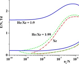
Figure 10. NDC region on the E/N–α plane for the He–Xe mixtures at N*/N = 0 [57].
Download figure:
Standard image High-resolution imageElectron collisions with excited atoms at a high δ change the shape of the EEDF. To take into account this effect the drift velocity of electrons is calculated as a function of the excitation degree δ = N*/N, which is defined as a fraction of Xe atoms in the lowest metastable level. In the absence of relevant experimental data for a rare-gas-mixture discharge, such an approach gives an idea about the opportunity to find conditions for NDC realization.
The authors of [58] have revealed that the Coulomb collisions can induce the NDC in pure rare gases (Ar, Kr, Xe) at a sufficiently high ionization degree α. These results are surprising since it was previously believed that the NDC occurs only in mixtures of rare gases possessing R–T minimum in qm with gases introducing electron energy losses [14, 41–42, 54–55]. Figure 11 shows W(E/N) dependences calculated for pure Xe for a few values of α and δ. The processes taken into account were the following: loss and gain of the electron energy in the elastic scattering from atoms, excitation of electronic states and ionization by electron impact from the ground state, stepwise excitation, second kind collisions with excited atoms, e–e and e–i collisions. It should be stressed that in pure Xe the NDC effect appears even at δ = 0 (curve 2 in figure 11). It can be explained by an influence of Coulomb collisions on the EEDF shape.
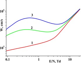
Figure 11. Electron drift velocities versus E/N in Xe, T = 300 K. (1) α = δ = 0; (2) α = 10−6 and δ = 0; (3) α = 10−6 and δ = 10−5.
Download figure:
Standard image High-resolution imageAt low energies, collisional energy relaxation at energy up to the R–T minimum in the momentum-transfer cross section is very slow. Therefore, at lower energies, the EEDF is almost constant. Due to the u−2 dependence of the Coulomb collision cross sections, e–e collisions are most effective at low electron energies. Hence, e–e collisions drive the EEDF toward the Maxwellian in the low-energy region. Then, this region with the quasi-Maxwellian EEDF extends to higher energy with α growing. This change in the EEDF shape is accompanied by diminishing mean energy, and the growth of W may be explained in two ways: as a result of an increase in the integrand (−(∂f0/∂u)) in formula (7) for W or due to decrease in qm at the mean energy (see figure 2). The NDC takes place, if the increment in W is greater at the lower electric field. Numerical calculations demonstrate that this is the case. According to our calculations, for a high degree of ionization, α = 10−5, the EEDF is close to the Maxwellian in the energy range of a few eV. This is also the range that contributes the most to the integral in (7). In this limit, W is a monotonically growing function of E/N.
Figure 11 demonstrates that in the presence of excited Xe atoms the NDC is more pronounced. Their role, because of the relatively low threshold for the stepwise excitation process Xe* + e → Xe** + e (1.16 eV), is similar to the role of molecular additives. The influence of second-kind collisions with excited atoms on the NDC was found to be insignificant [58].
By numerical calculations, the regions in the α–E/N parameter space were identified where the NDC exists. The calculations were made for Xe (figure 12), Kr and Ar (figure 13) [58].
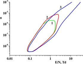
Figure 12. α–E/N diagram for Xe. Lines are bound regions where the NDC exists. (1) δ = 0; (2) δ = α; (3) δ = 10α [58].
Download figure:
Standard image High-resolution image
Figure 13. Region of the NDC effect in α–E/N space for Ar. (1), (2) δ = (0–α); (3) δ = 10α [58]; (1) e–i collisions neglected; (2), (3) e–i collisions included.
Download figure:
Standard image High-resolution imageIn figures 12 and 13 results for δ = 0, δ = α and δ = 10 α(δ is the fraction of atoms on lowest metastable state) are demonstrated. The populations of higher electronic states were neglected.
The role of electron–ion (e–i) collisions was also studied. It should be noted that in contrast to e–e collisions, where electron momentum is conserved, the e–i collisions cause a notable change in the electron momentum, while their impact on the electron energy distribution is much less. We therefore neglect electron energy change in the e–i collisions. The momentum-transfer cross section for the e–i collisions in Ar is about 10−11 cm2 at u = 0.25 eV resulting in the electron momentum relaxation rate of same order as at the electron–atom collisions at α = 10−7. Calculations show that for Xe and Kr, the role of e–i collisions can be neglected, while for Ar these collisions reduce the regions for NDC existence. To illustrate this effect, curve 1 in figure 13 relates to the case when e–i collisions were neglected. All other calculations were made including the effect of e–i collisions.
Let us discuss the data presented in figures 12 and 13 in more detail. We have found that NDC behavior at variation of α and δ is similar for Xe and Kr. Therefore, we focus our attention on the comparison between the NDC effect in Xe and Ar. The greater the electric field strength, the greater the characteristic electron energy and higher ionization degree is necessary for the e–e collisions to compete with the electron–atom collisions. The high sensitivity of the NDC effect to molecular additives makes it difficult to identify the NDC effect in pure Ar, Kr and Xe associated with the e–e collisions. The difference in the ranges of E/N where NDC can be observed (compare figures 12 and 13) is explained by the difference in positions of the minimum of the momentum-transfer cross section for Ar and Xe (see figure 2). The smaller size of the NDC region for Ar in comparison with Xe is due to more gradual growth of the momentum-transfer cross section with energy.
Comparison of figures 12 and 13 reveals a new unexpected feature: deformation of the NDC region with the increase in metastable state populations for Xe and for Ar proceeds in different ways. The broadening of the NDC region with N* growth for Xe can be easily explained by electron energy loss in stepwise excitation of atoms, which is similar to inelastic collisions with molecular species. To understand why the same collisions in Ar give opposite results, it is necessary to look at the processes in more depth. The R–T minimum for Ar is much deeper and located at a lower energy than for Xe. As a result, the e–i collisions come into play at much lower α, and effectively modify the momentum-transfer cross section near the minimum.
Let us discuss whether it is possible to experimentally observe the predicted NDC in pure rare gases. The EBSD allows one to change gas pressure, E/N and electric current density independently. The first observation of discharge current oscillation in the EBSD in 'pure' Ar [24] was explained by the authors as a manifestation of the Gunn effect. Our calculations for conditions of this experiment predict that the NDC exists at E/N < 0.6 Td. Estimations of E/N value from the measured discharge voltage and discharge spacing gave the E/N ≈ 5–6 Td. Such a discrepancy between predicted and estimated values of E/N might be explained by the presence of impurities in Ar.
It is well known [59] that in the glow discharge there exist regions with rather low electric field. These regions are the negative glow and the Faraday dark space. The electron kinetics in these regions is quite similar to electron kinetics in EBSDs. Ranges of plasma parameters where one may expect appearance of the NDC in pure Ar and Xe are shown in figures 10–13. Current oscillations associated with the NDC reflect formation of high-field layers in plasma, which propagate from the cathode layer to the anode. Conditions for their formation depend, among others, on the length of the plasma layer with the NDC. It means that the local existence of NDC is a necessary but not sufficient condition for the appearance of electric current oscillations.
The possibility of observing NDC phenomena in pure Xe, as induced by Coulomb collisions, is searched in detail by self-consistent numerical modeling [60]. The self-consistency of the model gives credence to the predictions. It was shown that the NDC can be observed experimentally in the EBSD in pure Xe provided the admixture of N2 concentration is lower than 10 ppm.
4. Absolute negative electron mobility
Conditions under which electron mobility in low-ionized plasma is negative are exotic. However, this effect is of fundamental interest providing an example of plasmas with unusual properties. This effect is also called negative electron drift velocity and absolute negative electron mobility or absolute negative conductivity (ANC) of plasma, provided the conductivity of plasma is controlled mostly by electrons. Evidently, the plasma with negative electron conductivity is unstable. In such a plasma electromagnetic waves are amplified. At present, several physical situations are known, in which the occurrence of negative electron mobility was theoretically studied: transient effect in decaying plasma in a course of EEDF relaxation, electron beam-sustained plasmas, plasma under steady-state Townsend (SST) conditions and photo-plasmas. Experimentally this effect was observed only in the case of the transient xenon plasma and is known as transient negative mobility [61].
Formal conditions necessary for the existence of the ANC were discussed in many papers and can be described as follows. Two equivalent formulae can be derived for the electron mobility:
The second expression can be derived by integrating the first one by parts. From the first formula, it follows that the electron mobility might be negative provided the derivative of function f0 is positive in a certain energy range (df0/du > 0, further this function is called 'the inverse function'). From the second formula, it follows that the condition d(u/qm(u))/du < 0 should be satisfied. In other words, qm(u) should be a super-linear function of energy. Evidently, both conditions are necessary but not sufficient for the electron mobility to be negative.
In the simplest case, when f0(u) can be approximated by the delta function located at an energy value, where condition d(u/qm(u))/du < 0 is true, the electron mobility is evidently negative. For convenience, electrons can be divided into two groups: (1) moving against the electric field; (2) moving along the electric field. Electrons in the first group gain energy from the electric field. Since the cross section qm(u) increases sharply with energy, the elastic collision frequency for these electrons grows, and the velocity direction is quickly randomized resulting in diminishing mean velocity against the electric field. Electrons in the second group lose their energy. Elastic collision frequency for these electrons decreases as a function of their energy, and the mean velocity along the electric field grows. As a result, conditions may be reached when the average electron velocity is along the electric field, i.e. the electron mobility is negative.
The condition d(u/qm(u))/du < 0 is satisfied, for example, for transport cross sections for Ar, Kr and Xe in the energy range above the R–T minimum (see figures 2 and 14). As for the condition df0/du > 0, the inverse distribution function can form under various physical conditions: in plasma of heavy rare gases during EEDF relaxation, in steady or decaying plasmas of heavy rare gases with electronegative admixture (due to the elimination of low-energy electrons by attachment processes) and in optically excited plasma of heavy rare gases with admixture of metal atoms (due to the second kind collisions of electrons with excited metal atoms). In figure 15 cross sections for the electron attachment to CCL4, F2 and NF3 molecules are shown, these gases were considered as admixtures in studies of negative mobility.
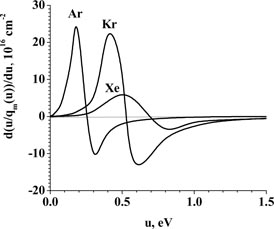
Figure 14. Derivative d(u/qm(u))/du calculated for Ar, Xe and Kr. The cross section data were taken from [36].
Download figure:
Standard image High-resolution image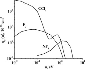
Download figure:
Standard image High-resolution image4.1. Transient negative mobility
This terminology corresponds to the situation when the variation of the EEDF shape is much faster than the variation of the electron number density. To the best of our knowledge, the transient negative electron mobility was introduced for the first time in [65, 66]. In these papers the time evolution of the EEDF in an electric field in Ar, Kr and Xe was studied theoretically for the limiting case when the initial EEDF was approximated by the delta function located at a given energy u0. It was shown that at the appropriate choice of u0 the negative electron mobility in xenon appears within a short time interval. Later [67], a similar effect was predicted in calculations of the EEDF relaxation in Ar plasma after switching off the external electric field. In contrast to papers [65, 66], the EEDF at the switching off moment was taken in [67] equal to the steady-state EEDF in the initial external electric field. In this case, the initial f0(u) is not the inverse one, and the inverse EEDF is formed in the course of the relaxation process. It was demonstrated that for the electric field E/N ⩾ 0.15 Td electron mobility in argon is negative in a time interval during EEDF relaxation.
The author of [67] performed calculations for Ar and indicated that the transient negative electron mobility should take place in Kr and Xe, as well. Calculations for Xe were performed in [68, 69], and it was shown that after the electric field stepwise switching from relatively high (5 Td, 1 Td) to a low (0.01 Td) E/N value there exists a time interval where the electron drift velocity is negative. Transient negative electron mobility in Xe was also predicted in [70], where initial EEDF was assumed to be a narrow Gaussian distribution with a center at u = 15 eV.
To illustrate the situation described above we have calculated the time variation of the EEDF in homogeneous low-ionized Ar plasma under conditions when the electric field is switched by a single step from E/N = 1 Td to E/N = 0.01 Td. Calculations were performed by numerically solving time-dependent BE. The following processes were taken into account: loss and gain of the electron energy in the elastic scattering from atoms and excitation of electronic states. The momentum-transfer cross section was taken from [36] and cross sections for the excitation of electronic states were taken from [71]. Electron concentration was assumed to be constant during EEDF relaxation and quite low, so the Coulomb collisions were not taken into consideration. The calculated EEDF is shown in figure 16 for various time moments. In the course of evolution, the shape of the EEDF changes significantly. There exists a large time interval where f0(u) is the inverse one. To give an explanation for this effect let us recall that the qm for Ar atoms increases in magnitude in the energy interval 0.25–10 eV (figure 2). At the initial moment, many electrons have relatively high energies (>1 eV). These electrons gradually lose their energy in elastic collisions, and, as a result, the probability of the elastic scattering falls down, which means a decrease in the rate of energy losses. For this reason, the flux of electrons along energy axis from high to low energies results in the formation of the inverse EEDF. Figure 17 shows the calculated electron drift velocity as a function of time. One can see that the drift velocity is a non-monotonic function of time and becomes negative within a time interval (0.06–0.35 ms).
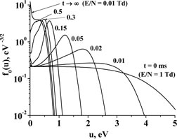
Figure 16. Calculated evolution of the EEDF in Ar, P = 1 Torr, T = 300 K. Time is measured in ms, t = 0 is the moment of the electric field switching down from E/N = 1 Td to E/N = 0.01 Td.
Download figure:
Standard image High-resolution image
Figure 17. Calculated evolution of the electron drift velocity in Ar, P = 1 Torr, T = 300 K. t = 0 is the moment of the electric field switching down from E/N = 1 Td to E/N = 0.01 Td.
Download figure:
Standard image High-resolution imageThe influence of e–e collisions on the EEDF shape and the value of transient electron mobility was studied in [68] for the case of Xe. It was shown that the transient negative mobility could be realized at the ionization degree of plasma α ⩽ 10−8.
In experiments [61], the ANC was detected on a nanosecond time scale in relaxing Xe plasma (gas pressure P = 20 atm) produced by a short (10 ns) x-ray pulse (figure 18). Electric field applied across the plasma was as low as 1.16 × 10⁻³ Td. The observed effect was explained in terms of transient negative electron mobility [72]. It was shown that the behavior of the measured plasma conductivity and calculated μe(t) as functions of time are rather similar in a case when the initial f0(u) in calculations is taken as a delta function at u0 = 0.864 eV.

Figure 18. The conductivity of xenon plasma (P = 20 atm) produced by 10 ns x-ray pulse (experiment [61]). The end of the x-ray pulse is at t = 0.
Download figure:
Standard image High-resolution imageIn paper [73] transient ANC was theoretically predicted for Xe : Cs mixtures. The authors suggested ionizing Cs atoms by a laser pulse with an appropriate wavelength, which is simpler than an x-ray pulse.
4.2. Absolute negative conductivity in steady-state EBSD
Figure 15 demonstrates that in some electronegative gases the electron attachment rate grows at lower electron energy. Such behavior is beneficial for the formation of the inverse EEDF and to the ANC. Experimental conditions for the appearance of the ANC are expected to be realized in the EBSD in rare gases with admixtures of electronegative gases such as those shown in figure 15. A number of papers are devoted to searching conditions for realization of the ANC in the EBSD (Ar : CCl4 [74, 75], Ar : F2 [76–78] and Xe : F2 [79–80]).
Electron energy spectrum in a gas irradiated by a beam of fast electrons stretches from zero to the energy of fast electrons. The low-energy range of this spectrum, i.e. the range of energies from 0 to ionization potential of atoms or molecules (I), is of a particular interest to finding conditions for the ANC. Respectively, in this subsection the term EEDF will be used precisely for this range of the electron energy spectrum. For uniform and steady-state plasma BE for the EEDF can be written as

The term qS(u) is the source of electrons in the energy range 0 ⩽ u ⩽ I with a spectrum
 and total production rate q. This term accounts for ionization of atoms and molecules by fast electrons.
For the first time, the inverse EEDF and the negative plasma conductivity in the EBSD were theoretically predicted in [74–75] for the case of the Ar : CCl4 mixture. The EEDF and plasma parameters were calculated by solving equation (10) by taking into account loss and gain of the electron energy in the elastic scattering from atoms and molecules, inelastic processes (excitation of electronic states of Ar atoms and CCL4 molecules, electron attachment to CCL4 molecules) and electron–electron collisions. Spectrum S(u) was calculated using a fast electron degradation spectrum in argon [81]. The main channel in plasma electron losses is electron attachment to CCl4 molecules. The EEDF and electron concentration were calculated in a self-consistent manner.
It was shown in [74] that, under certain conditions, the EEDF in Ar + 0.1% CCl4 plasma is inverted, but the possibility of the existence of negative plasma conductivity was not discussed. The ANC in the EBSD was then studied in [75] for the same gas mixture. Figure 19 shows the EEDFs calculated in [75] for various q values at E/N = 0. One can see that EEDFs have the pronounced maximum at energies ∼1.5 eV. A decrease in f0(u) in the energy range u < 1.5 eV is explained by the electron attachment to CCl4 molecules. Calculated electron drift velocity and electron current density as functions of E/N value are shown in figures 20(a) and (b). One can see that electron drift velocity and current density are negative in the range of E/N from 0 to a certain value, which depends on the partial concentration of CCl4 molecules and on the production rate of electrons. As the electric field increased, the negative electron mobility vanishes. This effect can be explained by a flattening of the EEDF with electric field growth.
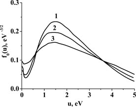
Figure 19. Steady-state EEDFs in Ar+0.1% CCl4 plasma (P = 3 atm, T = 300 K, E/N = 0) sustained by a beam of fast electrons calculated for various production rates q [75]. (1) q = 1.3 × 1021 cm−3 s−1; (2) 3.9 × 1021 cm−3 s−1; (3) 1.3 × 1022 cm−3 s−1.
Download figure:
Standard image High-resolution image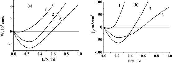
Figure 20. Electron drift velocity (a) and electron current density (b) as functions of E/N calculated in Ar + 0.1% CCl4 plasma (P = 3 atm, T = 300 K) sustained by a beam of fast electrons [75]. (1) q = 1.3 × 1021 cm−3 s−1; (2) 3.9 × 1021 cm−3 s−1; (3) 1.3 × 1022 cm−3 s−1.
Download figure:
Standard image High-resolution imageIn the Ar : CCl4 discharge, negative ion number density can essentially exceed electron number density. Plasma conductivity is negative, if the negative electron current exceeds (by magnitude) positive and negative ion currents. According to our estimations for the conditions of curves 2 and 3 in figure 20(b) at E/N < 0.4 Td conductivity of plasma is negative. This prediction is not yet verified experimentally.
In conclusion, so far there was no experimental observation of negative electron conductivity in the EBSD. In [82] the electron number density was measured by laser interferometry at wavelength 9.6 µm in Ar : F2 electron beam-sustained discharge in a wide range of parameters (percentage of F2 admixture, electron beam current density and applied electric field). The electron drift velocity values were calculated as a ratio of the discharge current to electron number density and the elementary charge. These measurements showed that electron drift velocity is positive in the whole range of parameters under study. In [77] the range of parameters for the existence of ANC in Ar : F2 EBSD was theoretically determined and compared with that considered in [82]. It was found that the predicted region of the ANC appearance on a plane (ne, %F2) touched closely the region with experimental data but had no common part. The authors of [78] revealed that the appearance of the ANC for Ar : F2 is very sensitive to the shape of the Ar transport cross section. Using two different versions of Ar transport cross sections ([36] and [83]), in the first case, the ANC existence was predicted, while in the second case the ANC was absent at the same EBSD parameters. Present analysis with Ar transport cross sections from [36] allows us to conclude that in a whole range of ne, %F2 parameters explored experimentally [82] showed the ANC does not exist.
In [84] the negative electron mobility was predicted for pure Xe EBSD. The authors claimed that the steady-state inverse EEDF is formed due to the dissociative recombination of low-energy electrons with
 ions. In the following paper [75] it was shown that taking into account e–e collisions results in the disappearance of the ANC under conditions studied in [84]. It is noteworthy that the omission of e–e collisions in the model of [75] leads to the appearance of the ANC under conditions analyzed in [84].
4.3. Negative electron mobility in decaying plasma
This subsection is devoted to studies of decay of homogeneous plasma of heavy rare gas with electronegative admixture in the presence of external electric field. The initial electron and positive ion densities are taken equal to each other. Plasma with such initial conditions can be created by a short ionizing pulse. If the applied electric field on the post discharge phase is sufficiently low, the rate of electron attachment to electronegative molecules is higher than the ionization rate, so plasma starts to decay. In this case, electron density is decreasing and, simultaneously, the EEDF shape deviates from the initial one.
In this case, it is convenient to analyze the evolution of function F(u, t) = ne(t)f0(u, t) with the initial condition F(u, 0) = ne(0)f0(u, 0). In a plasma decaying in a steady-state electric field, after a certain time interval, the EEDF shape is established, and electron number density exponentially diminishes with time. As a result, the function F(u, t) is factorized as F(u, t) = ne(t) × f0(u), where ne(t) ∼ exp(−νatt), and νat corresponds to the attachment frequency calculated from the established f0(u). Such a scenario for F(u, t) evolution was confirmed in [78, 85–88]. For a given E/N, f0(u) and νat do not depend on the initial conditions. It was shown that under certain conditions established f0(u) has the inverse form, and electron mobility is negative (Ar : NF3 [85, 86], Ar : F2 [78, 87, 88]). Various mathematical techniques were implemented in these studies: solving the BE in two-term approximation [78, 85–87]; Monte Carlo simulations [87] and solving the BE in the eight-term approximation for the distribution function [88].
It is worth mentioning [89, 90], where the role of negative electron mobility under RF electric field conditions was studied by the Monte Carlo method in decaying Ar : F2 plasma.
For illustration purposes, figures 21 and 22 show the established f0(u) and drift velocity in decaying Ar : F2 = 1 : 0.005 plasma calculated in [87] by solving the BE. In the computations, the following processes were taken into consideration: loss and gain of the electron energy in the elastic scattering from atoms and molecules, the excitation of the vibrational levels and electronic states of F2 molecules; and the electron attachment to F2 molecules. Figure 22 demonstrates quite unexpected behavior W as a function of E/N. An increase in drift velocity in the range E/N from 0.01 to 0.053 Td is followed by an abrupt transition from a positive value at 0.053 Td to a negative one at 0.055 Td. In the range from 0.055 to 0.55 Td the drift velocity is negative, and its minimum value is about −5 × 10⁴ cms−1. For E/N > 0.55 Td the drift velocity becomes positive again and increases with E/N.

Figure 21. The established distribution function f0(u) in a decaying Ar : F2 = 1 : 0.005 plasma [87]. T = 300 K, P = 1 atm. (1) E/N = 0.04 Td, (2) E/N = 0.07 Td, (3) E/N = 0.1 Td, (4) E/N = 0.5 Td, (5) E/N = 1 Td.
Download figure:
Standard image High-resolution image
Figure 22. The established electron drift velocity as a function of E/N in a decaying Ar : F2 = 1 : 0.005 plasma [87]. T = 300 K, P = 1 atm.
Download figure:
Standard image High-resolution imageSuch an unusual dependence of electron drift velocity on the electric field was explained in [86, 87] in the following way. The plasma electrons can be divided into two groups: electrons with energies u < um, where um = 0.08 eV is the energy at which the electron attachment cross section is maximum (see figure 15) and electrons with energies u > um. Particle exchange between these groups proceeds through a number of collisions resulting in high probability for the electron to be attached. As the plasma decays, the electron density in every group decreases almost independently, and the shape of the established distribution function f0(u) is governed by the ratio between the decay rates of these electron populations. If the electric field is weak, the rate of the electron loss in the first group is low since the attachment cross section is small in the low-energy range. Owing to elastic and inelastic collisions the energy of electrons from the second group becomes lower than 0.4 eV. Since the attachment cross section is large in the energy range um < u < 0.4 eV the electron loss rate is very high. As a result, the established f0(u) is governed by electrons from the first group. In this case f0(u) is a monotonically decreasing function (see curve 1 in figure 21). The corresponding value of the electron drift velocity is positive.
As the electric field increases, the mean electron energy grows and the attachment for the electrons from the first group rises, since the attachment cross section increases with energy in the range u < um. For E/N > 0.55 Td the rate of electron loss for the first group is higher than that for the second group. In this case, the established f0(u) is mainly governed by the electrons from the second group and has an inverse form (see curves 2–3 in figure 21). As a result, drift velocity becomes negative. With further electric field increase the electrons from the first group acquire sufficient energy (during their lifetime) to overcome the attachment barrier in the energy space. In this case, a weakly inverse or monotonic function f0(u) is formed (see curves 4–5 in figure 21), and the drift velocity becomes positive.
In decaying plasmas, the electron number density falls down because of the electron attachment to molecules. Hence, the total negative plasma conductivity can be observed provided the electron number density is sufficient for dominance of electron current component. Moreover, it was shown in [78] (for Ar : F2) and [86] (for Ar : NF3) that evolution of the EEDF shape is rather sensitive to the detailed shape of the initial EEDF, f(u, 0). It was concluded that the best way to observe the negative plasma conductivity in experiments is to use a high-voltage short pulse in order to form the initial EEDF with a high temperature.
4.4. Negative electron mobility under SST conditions
In a SST experiment a steady flux of electrons is emitted from the cathode and electrons move in the uniform electric field between electrodes. The electron concentration and the shape of the EEDF change with distance from the cathode. In the case of electronegative gas and sufficiently low electric field strength electron concentration decreases with distance due to attachment of electrons to electronegative molecules. The space variation of function F(u, x) = ne(x)f0(u, x) can be found by solving the steady-state BE with the boundary condition F(u, 0) = ne (0)f0(u, 0). In this case, the EEDF shape is established at some distance from the cathode, the function f(u, 0) is factorized, and the electron number density falls down exponentially with coordinate x:

Here γat is the attachment coefficient at the established EEDF shape. Such a scenario for F(u, x) spatial evolution was predicted in [91] by Monte Carlo calculations.
In this limit, the energy dependent factor, f0(u), satisfies the steady-state BE for the function [92]:
Integrating (12), the following equation for the attachment coefficient reads

Here Nat is the number density of an electronegative additive, kat is the attachment rate coefficient.
By solving equations (12) and (13) it was shown [91] that in an Ar : NF3 mixture under SST conditions the inverse EEDF can be formed and electron mobility can be negative (see figures 23, 24). The following processes were taken into account in calculations: loss and gain of the electron energy in the elastic scattering from Ar atoms and NF3 molecules, the excitation of the electronic states of Ar atoms, the excitation of the vibrational levels of NF3 and the attachment of electrons to NF3 molecules.

Figure 23. The established EEDF calculated for Ar : NF3 mixture under SST conditions [91]. T = 300 K, P = 10 Torr, E/N = 0.1 Td. [NF3] = 1% (1); 0.1% (2); 0.01% (3); 0% (dashed line).
Download figure:
Standard image High-resolution image
Figure 24. The established electron drift velocity W calculated for Ar : NF3 mixtures under SST conditions [91]. T = 300 K, P = 10 Torr, E/N = 0.1 Td. [NF3] = 1% (1); 0.1% (2); 0.01% (3).
Download figure:
Standard image High-resolution imageThe dip in the EEDF at low-energy (see figure 23) was explained in [91] as follows. For pure Ar the EEDF at low E/N is established as a result of exact compensation of forward and the backward flows of electrons along energy axis. The forward flow is due to energy gain in the electric field, and the backward flow is due to its loss in elastic collisions with atoms. The result is the monotonic EEDF (see dashed curve in figure 23). The NF3 admixture introduces the attachment process, the cross section of which has a maximum at an energy value of about 1.5 eV (see figure 15). It is instructive to consider the EEDF formation in vicinity of zero energy. Evidently, the heating of electrons by the electric field results in electrons moving these to a higher energy range. Both, electron heating by the electric field and elastic collisions are conservative processes with respect to electron number density. However, when electrons approach an energy value, where the attachment is probable, they disappear due to the attachment processes. This disturbs the balance of forward–backward electron flows along energy axis. Namely, the backward flow diminishes. Due to the conservative nature of the energy gain-loss processes, this leads to electron number density diminishing the with zero energy.
If the electron energy is relatively high, the probability of electron attachment is comparable, or higher, than the probability for removal of electrons from the energy interval by virtue of elastic collisions. As a result, the EEDF with a lack of low-energy electrons is formed. The location of the EEDF's maximum on the energy axis depends on both the value of the reduced electric field and the NF3 concentration.
It was also demonstrated that at all NF3 concentrations under analysis W is a non-monotonic function of E/N. Moreover, in all of the cases, a range of E/N parameter values exists where the drift velocity is negative (see figure 24). Under SST conditions the flux of electrons from the cathode to the anode is formed by two processes: drift and diffusion. The total electron flux is controlled by the so-called diffusion-modified drift velocity V = W + γatD (see [92–94]). The authors of [91] proved that V ⩾ 0 at all reasonable values of plasma parameters. In other words, the negative drift velocity W is compensated by the electron diffusion caused by descending spatial profile of electron number density. As a result, the plasma conductivity is positive.
4.5. Negative electron mobility in optically excited plasma
In experimental work [95] the Q-factor of a microwave resonator filled with a Xe : Hg : Cs : CO gas mixture was measured. The Q-factor was found to increase when the gas mixture was ionized by UV radiation. In [95], the increase in a Q-factor was attributed to the negative conductivity of the plasma created in the resonator. However, in [96] this statement was disproved.
In later papers [97–102] the possibility of negative electron mobility in optically excited plasma was analyzed theoretically by solving the BE. The following gas mixtures were considered: Na : Ar (Xe, Kr) [97, 98], Na : N2 : Ar (Xe, Kr) [98, 99], Li : N2 : Ar (Xe, Kr) [100–101]. In these papers, the EEDF and related plasma parameters were calculated for a high concentration of excited Na* (or Li*) atoms in plasma. The atom excitation degree, δ = [Na*]/[Na] (or [Li*]/[Li]), and ionization degree of plasma, α, were considered as independent parameters (except for paper [102]). The specific feature of the electron energy balance at low E/N values in these plasmas is that electrons gain the energy mostly in the second-kind collisions with excited atoms:


For a fixed excitation degree, processes (14) and (15) are steady sources of electrons with energies u > 2.1 eV and u > 1.8 eV, respectively. It was shown in [97–102] that in certain ranges of parameters (E/N, δ, α and the partial concentration of Na or Li atoms), calculated EEDFs are inverse ones, and electron mobility is negative.
The predicted effect exists at very low ionization degrees (a < 10−10–10−9) and this is in contradiction to the required high excitation degree of plasma (δ ⩾ 0.1). The possibility of the creation of steady-state plasma with such characteristics is rather slim. In [102], time evolution of electron concentration and conductivity in optically excited Li : N2 : Xe plasma was calculated starting from the exposure to radiation at zero electron concentration. It was shown that conductivity is negative at the earlier phase of the electron multiplication and becomes positive as soon as ne exceeds a certain value.
5. EEDF bi-stability
The EEDF bi-stability means that in plasma under the same conditions (gas number density, gas temperature, electric field strength) two stable states exist differing by the EEDF shape. The jump-like transitions between these two states proceed in a form of the instability development.
To give an idea about the origin of the EEDF bi-stability phenomenon let us consider a situation when the EEDF is Maxwellian: f0(u) = Cexp(−u/Te), where Te is the electron temperature and C is the normalization factor. In this case, the time-dependent equation for the electron temperature reads

Here H(Te) relates to electron heating by the electric field and by super-elastic collisions, L(Te) includes the loss of electron energy in elastic and inelastic collisions.
The number of steady-state solutions to equation (16) depends on the shape of the Φ(Te) function. In particular, if this function has an N-type shape shown in figure 25, then there exist three steady-state solutions to equation (16) (Te = T1, Te = T2 and Te = T3), two of which (Te = T1, Te = T3) are stable.
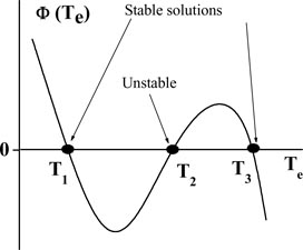
Figure 25. The shape of Φ(Te) function at which there are two stable solutions to equation (16).
Download figure:
Standard image High-resolution image5.1. EEDF bi-stability in plasma of heavy rare gases
For a limit of the Maxwellian EEDF, the bi-stability was predicted in [103] (see figure 26). An object of study in [103] was plasma of rare gases possessing R–T minimum in momentum-transfer cross sections. It was found that, in a certain range of E/N values, the right-hand side of equation (16) has three roots. Taking into account the striking similarity between the electron temperature behavior for Ar, Kr and Xe, further discussion concerns Xe gas. The respective H(Te), L(Te) and Φ(Te) functions calculated for pure Xe at E/N = 0.035 Td and gas temperature T = 300 K are shown in figure 27. The Φ(Te) curve is just of the type shown in figure 25. The N-type curve for H(Te) in figure 27 is a result of crossing two wavy curves for L(Te) and Φ(Te) functions. Wavy behavior in the opposite direction of L(Te) and Φ(Te) curves is explained by variation of qm around R–T minimum. The point is that L(Te) is proportional to qm(u), while H(Te) varies proportionally to [qm(u)]−1. The competition between these two terms derives the bi-stability phenomenon.
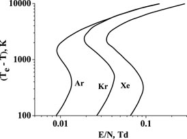
Figure 26. Electron temperature in Ar, Kr and Xe as functions of E/N parameter [103].
Download figure:
Standard image High-resolution image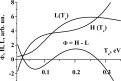
Figure 27. H(Te), L(Te) and Φ(Te) functions calculated for pure Xe at E/N = 0.035 Td and T = 300 K.
Download figure:
Standard image High-resolution imageIn [104] the bi-stability effect was predicted for positron swarms in He. The positron energy distribution function was approximated by the Maxwellian one.
In fact, approximation of the realistic EEDF by the Maxwellian can be approved under rather specific conditions. Evidently, just e–e collisions drive the EEDF to the Maxwellian function. Moreover, e–e collisions introduce non-linear terms into the BE [2]. It seems probable that this non-linearity may result in the appearance of the bi-stability effect. A possible way to find numerically different stable solutions to the BE at fixed plasma parameters is to solve time-dependent BE (relaxation method) with different initial f0(u). If the iteration method is used to solve steady-state BE, then different initial f0(u) should also be exploited. It is convenient to take as an initial f0(u) the Maxwellian with a given electron temperature Te0, with the following variation of its value in a series of calculations.
The bi-stability effect in plasma of heavy rare gases was studied in [105] by solving the BE by taking into account loss and gain of the electron energy in the elastic scattering from atoms, excitation of electronic states by electron impact and e–e collisions. This effect was revisited by numerically solving the BE [106, 107] with the use of updated data on momentum-transfer cross sections [36]. It follows from [105, 106] that, in a certain range of parameters (namely, the reduced electric field, E/N, and the degree of ionization, α), the BE has two stable solutions. It means that in such a plasma two different steady states with different plasma parameters can be realized.
The EEDFs in Xe plasma calculated at E/N = 0.035 Td and different α values [107] are shown in figure 28. According to calculations, for 10−7 > α > 10−10 there are two stable solutions to the BE. Let us note that for the ionization degree α = 10−9 two calculated f0(u) functions (curves 3 and 3' in figure 28) differ markedly from the Maxwellian, while for α = 10−7 EEDFs are close to the Maxwellian.
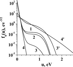
Figure 28. EEDFs in Xe plasma [107] calculated at E/N = 0.035 Td and T = 300 K (1) α = 0, (2) 10−10, (3),(3') 10−9, (4),(4') 10−7. Reprinted with permission from [107]. Copyright 2006, AIP Publishing LLC.
Download figure:
Standard image High-resolution imageElectron drift velocity in pure Kr and Xe calculated at low electric fields are shown in figures 29(a) and (b), respectively. As follows from these figures, bi-stability effect takes place for a > 10−10 in the E/N intervals E/N ≈ 0.027–0.043 Td (Xe) and E/N ≈ 0.01–0.015 Td (Kr).
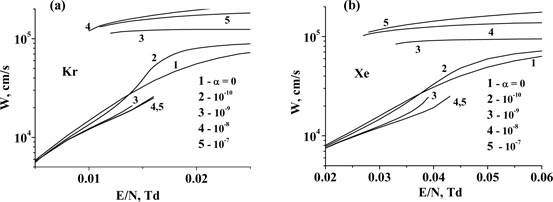
Figure 29. Electron drift velocity in Kr (a) and Xe (b) calculated for different ionization degrees [106]. T = 300 K.
Download figure:
Standard image High-resolution imageElectric field strengths where the bi-stability effect has been found are rather low, so that the rate of electron-impact ionization is negligible under bi-stability conditions. Experimentally, such conditions can be realized, for example, in decaying plasma in the low electric field. In [103] the time variation of the current in xenon afterglow plasma with applied probing electric field was measured. It was observed that at some point there is a jump-like decrease in the current value (t = 0.6 ms, see figure 30). The authors of [103] consider this abrupt decrease as the manifestation of the bi-stability effect.

Figure 30. Electric current as a function of time in xenon afterglow. P = 2.3 Torr, probing electric field E/N ∼ 0.01 Td [103].
Download figure:
Standard image High-resolution imageIn the alternating electric field the bi-stability leads to hysteresis in cyclic time variation of electron drift velocity (and, respectively, current). In [106] the electron drift velocity in Xe under the influence of the alternating electric field was studied by numerically solving time-dependent BE. The amplitude of the electric field (E0 = 0.06 Td at P = 1 Torr and T = 300 K) was chosen in order to cover the E/N interval in which bi-stability takes place (see figure 29(b)). Under these conditions ne varies slowly in comparison with the electric field variation, and the ionization degree was taken as a time-independent parameter.
Figure 31 shows the established time variation of the electron drift velocity within half a cycle, calculated for P = 1 Torr, α = 10−8 and different electric field circular frequencies, ω. It is seen that for ω ⩽ 103 rad/s an abrupt increase in drift velocity took place at the cycle phase ω t ≈ 0.35π at growing electric field. This abrupt increase corresponds to the transition from the lower to upper branch of We(E/N) dependence, when E/N reaches a value about 0.042 Td (see curve 4 in figure 29(b)). The transition from the upper to lower branch of W(E/N) dependence, which occurs when decreasing electric field reaches a value of about 0.025 Td, is remarkably smooth and does not have any peculiarities. It was pointed out in [106], that the difference between lower-to-upper and upper-to-lower transitions is explained by the specific shape of the momentum-transfer cross section of Xe.

Figure 31. Established variations of electron drift velocity with time in pure Xe. P = 1 Torr, T = 300 K, α = 10−8, E(t)/N = 0.06*sin(ωt) [Td].
Download figure:
Standard image High-resolution imageAccording to our estimations, under considered conditions effective frequency of the EEDF relaxation, νu, is about 2 × 10³ s−1. If the electric field frequency ω≫νu (and ω ≪ νm), then the EEDF and electron transport coefficients vary slightly within the period, and their values averaged over the period are close to those in the steady the electric field with
 [108]. If the effective
 value is that at which bi-stability takes place, then there could be two different solutions to time-dependent BE at ω ≫ νu. Calculations performed for Xe (P = 1 Torr, T = 300 K, α = 10−8) under alternating electric field conditions E(t)/N [Td] = 0.05*sin(ωt) show that at ω < 2 × 10³ rad/s there is a unique established solution to time-dependent BE. At ω > 2 × 10³ rad/s two different established dynamic solutions are observed. To illustrate this fact, figure 32 shows the calculated mean electron energy (averaged over a period) as a function of the electric field frequency. It is noteworthy that under alternating electric field bi-stability appears just at the electric field frequency about the frequency of the EEDF relaxation, ω ∼ νu.
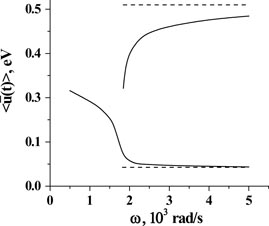
Figure 32. Averaged over a period, mean electron energy as a function of electric field circular frequency (solid lines), Xe, P = 1 Torr, Tg = 300 K, α = 10−8, E(t)/N = 0.05*sin(ωt) [Td]. The dashed lines show limit values corresponding to effective electric field
 .
.
Download figure:
Standard image High-resolution imageIn the studies described above the electron number density was considered as an independent parameter. Since the bi-stability effect has been found at rather low electric fields, the situation considered can be realized in the decaying plasma or in non-self-sustained discharge. This opportunity was examined in [109, 110], in which the EEDFs in plasma of steady-state EBSD in heavy rare gases (Xe [109] and Ar, Kr [110]) were calculated.
The BE for the EEDF in plasma of steady-state EBSD was discussed in section 4.2. Under conditions considered in [109, 110] the secondary electrons lose their energy in elastic and inelastic collisions and disappear when recombining with positive molecular ions (
,
 ,
,
 ), which are the dominant ions in plasma. In [109, 110] recombination processes were taken into account in BE, and the EEDF and the electron concentration were calculated in a self-consistent manner.
It was found for Xe [109] and Kr [110] that in a certain range of q (production rate of electrons in the energy range 0 ⩽ u ⩽ I) and E/N values two different stable plasma states exist, the effect is more pronounced in the case of Xe. For an Ar plasma [110], the BE has a unique solution over the entire parameter range under study.
Figure 33 demonstrates calculated mean electron energy and plasma electron current density for non-self-sustained discharge in Xe at atmospheric pressure as functions of E/N [109]. Within the interval of q values 1014 cm−3 s−1 < q < 1017 cm−3 s−1 the bi-stability is clearly seen. The difference in discharge currents in the bi-stability range is almost ten-fold, and can be easily measured by common diagnostics. Production rate q = 1016 cm−3 s−1 corresponds to the electron beam current density ≈2µAcm−2 with the energy of fast electrons ∼300 keV [109]. The electron beam with such parameters can be easily realized.
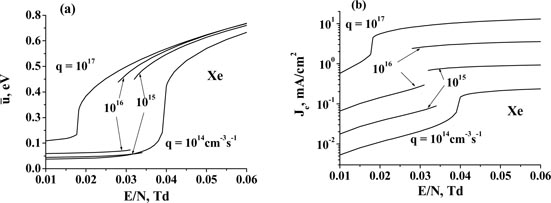
Figure 33. Plasma parameters in EBSD in Xe (P = 760 Torr, T = 300 K) [109]. (a) Mean electron energy, (b) electron current density.
Download figure:
Standard image High-resolution imageA possible experimental study is to measure the ampere–volt characteristics of the EBSD in Xe under described conditions. The required magnitudes of the voltage applied across the discharge gap should provide the E/N values in the range 0.01–0.06Td. When the bi-stability exists, the hysteresis effect should be observed manifesting itself as stepwise changes of the discharge current at certain values of the discharge voltage.
5.2. EEDF bi-stability in Ar : N2 post discharge plasma
In [111] an unusual time variation of the electron temperature in Ar+1% N2 post discharge plasma was observed (see curves 2 and 3 in figure 34) and an explanation was given in terms of the EEDF bi-stability effect.

Figure 34. (a) Experiment [111]. Electron (open circles) and vibrational (solid circles) temperatures in the afterglow. (b) Calculated time dependence of electron density [111]. Ar + 1% N2, P = 0.5 Torr, T = 300 K. Pulse current I = 700 mA (1), 500 mA (2), 200 mA (3).
Download figure:
Standard image High-resolution imageIn experiments [111] the discharge ran in a cylindrical tube of 3 cm diameter in a pulse repetition mode with pulse current I = 200–700 mA. Pulse duration was 40µs, and the pulse repetition frequency was 1 kHz. The EEDF and the vibrational temperature, Tv, of N2 molecules were measured at various delay times after the discharge pulse. The electron temperature was estimated from measured EEDF. Moreover, the time dependence of the electron concentration was estimated. Results of measurements performed at P = 0.5 Torr are shown in figure 34. It was found that measured Tv value is almost independent of pulse current and no noticeable decrease in Tv occurs during the post discharge period. In contrast, the electron temperature evolution strongly depends on the value of pulse current. For the pulse current 700mA Te gradually decreases with time (see curve 1 in figure 34(a)). At lower pulse currents a rather sharp bend appears in the Te(t) curves (curves 2 and 3 in figure 34(a)).
A specific feature of the EEDF formation in nitrogen (and nitrogen containing gas mixtures) afterglow is that heating of electrons is due to the super-elastic collisions of electrons with vibrational-excited molecules [11, 112–118]. Then it is the strong coupling between the vibrational excitation degree of the nitrogen molecules and the EEDF shape. For this reason, at first thought the jump-like Te(t) variation is in contradiction with the constant Tv(t) value (see figure 34(a)). The conditions under study in [111] are quasi-stationary for the formation of the EEDF. Therefore, the origin of Te(t) changing is the variation of the plasma parameters influencing it. Of these parameters only electron number density shows noticeable time dependence in the afterglow (see figure 34(b)). The ne value determines the frequency of e–e collisions, and these processes influence the EEDF formation in the afterglow plasma (see, for example, [116]).
A theoretical study [111] was made by numerically solving the steady-state BE for the EEDF. The following processes were taken into account: loss and gain of the electron energy in the elastic scattering from atoms and molecules, excitation and de-excitation of rotational, vibrational and electronic states of nitrogen molecules by electron impact, and e–e collisions. The distribution of nitrogen molecules over vibrational levels has been supposed to be a Boltzmann one with a given temperature Tv. The electron concentration was taken as an independent parameter. The population of all electronically excited states except
 was neglected. Some results of calculations are shown in figures 35(a) and (b).

Figure 35. Theory [111]. (a) Electron temperature in a post discharge as a function of ne, (b) two different EEDFs in a post discharge. Ar+1% N2, P = 0.5 Torr, T = 300 K,
![$[{\rm N}_{2}(A^{3}\Sigma _{{\rm u}}^{+} )]=10^{10\,}{\rm cm}^{-3}$](https://content.cld.iop.org/journals/0963-0252/23/4/043001/revision1/psst495639ieqn011.gif) .
.
Download figure:
Standard image High-resolution imageFor a given Tv the calculated Te strongly depends on the electron concentration (see figure 35(a)). In the case of high electron concentrations Te is close to Tv and slightly decreases as ne falls down. Then the sharp transition from high to low Te takes place at some critical ne value. The lower the vibrational temperature the higher the critical ne value and the more abruptly the transition occurs. Moreover, for lower Tv (for example, Tv = 3000 K, see figure 35(a)) the range of ne exists, in which there are two different stable solutions to the BE (see figure 35(b)). The possibility of bi-stability appearance is connected with comparatively narrow maximum in the cross sections for energy exchange between electrons and molecular vibrations.
Electron density decays in the afterglow. Then the jump-like Te(t) variation observed in experiments can be explained as a transition from high to low Te values after the electron density falls down to some critical value. The experimental results described can be considered as implicit evidence of the possibility of the bi-stability effect in Ar : N2 afterglow plasma.
The possibility to the observe the bi-stability effect in pure nitrogen afterglow plasma was discussed in [117–119].
6. Thermo-current instability
The thermo-current instability manifests itself in a form of plasma waves propagating along the electric field, which involve self-consistent variations of electron number density and electron temperature (see [120]). Such a phenomenon can take place in weakly ionized plasma under the external permanent electric field. An essence of this instability can be explained in simple terms for conditions when the wavelength of the plasma perturbation is much larger than the electron energy relaxation length, λu. Under this condition, the electron diffusion flux is negligible in comparison with the electron drift. Then, in the first order, the electric current continuity equation has a form

where x is the coordinate along the electric field. Let us consider the evolution of the local electron number density fluctuation (see figure 36). For a strictly increasing function W(E/N) the electric field strength and electron number density change in opposite directions, while the electron temperature follows the electric field strength. In this case, the electron thermo-diffusion flux induced by the gradient of the electron temperature Te, jTD ∼ ∂Te(x)/∂x, is directed opposite to the electron diffusion flux. Under condition |jTD|>|jD|, the plasma perturbation is enhanced.

Figure 36. Diagram illustrating the development of thermo-current instability [120].
Download figure:
Standard image High-resolution imageTo the best of our knowledge, such an instability was considered for the first time in [121], where the set of continuity equations for electrons and ions


was analyzed in the long-wavelength limit k−1≫λu (where k is the perturbation wave number) under the assumption of plasma quasi-neutrality. In equations (18) and (19), DL is the longitudinal electron diffusion coefficient [122, 123], Wi is ion drift velocity, ni is ion number density. It was shown in [121] that instability develops if the following condition is satisfied:

Using the results of [121], one can show that in the long-wavelength limit the instability growth rate Γ is proportional to k2.
Actually, electron number density and electric field strength longitudinal gradients are coupled according to the electric current continuity law. The authors of [124] took into account both these gradients self-consistently and derived a more general criterion for the onset of thermo-current instability in the limit of long perturbation wavelengths. Application of this criterion to different gases showed that the thermo-current instability can take place in helium (4 Td < E/N < 7 Td) [124]), nitrogen (0.07 Td < E/N < 0.2 Td and 70 Td < E/N < 130 Td) [125]) and carbon dioxide (7 Td < E/N < 23 Td) [126]). It was found that for He and CO2 [126, 127], Coulomb collisions and super-elastic collisions with vibrationally excited molecules narrow the E/N-range with thermo-current instability. The authors of [125] have found numerically that a magnetic field, H, impressed transverse to the electric field, appreciably changes the shape of the instability existence region on (E/N–H/N) plane. Figures 37 and 38 illustrate the E/N-range with thermo-current instability changes induced by variations of the ionization degree and of the reduced magnetic field strength, H/N, in He plasma.

Figure 37. The thermo-current instability region computed for He plasma by taking into account Coulomb collisions [127].
Download figure:
Standard image High-resolution image
Figure 38. The thermo-current instability region computed for He plasma in crossed electric and magnetic fields [125]. α = 0.
Download figure:
Standard image High-resolution imageIn [128, 129], thermo-current instability was studied using a set of transport equations, including the balance equation for the mean electron energy. However, this approach would be correct, if only the EEDF were Maxwellian. In a weakly ionized plasma, the EEDF differs from the Maxwellian, and the application of such an approach is unjustified.
The approach based on transport equations is applicable to the description of the thermo-current instability under condition k−1 ≫ λu [121, 124]. This theory predicts for quasi-neutral plasma the unlimited growth of the instability increment at short-wavelength perturbations, Γ ∼ k2. It was shown in [124] that the local disturbance of plasma quasi-neutrality dumps the thermo-current instability. Evidently, the EEDF variation on a spatial scale shorter than λu is negligible. One may expect that perturbation growth rate is maximum at k−1 ∼ λu. It means that a kinetic theory is required to describe the thermo-current instability around maximum of its increment.
For the first time, the kinetic approach was used to develop the small-perturbation theory of thermo-current instability for a model gas in [130]. Then, in [131], the same approach was used to describe numerically the linear stage of this instability in helium. In [130, 131] the plasma was assumed to be quasi-neutral. Recently, in [120], kinetic approach was utilized to calculate instability growth rate in a model gas with allowance for disturbance of plasma neutrality in perturbations.
In [120, 130, 131] the BE for the spherically symmetric part of the EEDF in an inhomogeneous plasma (3) in combination with ion continuity equation (19) was implemented.
In [120, 130] a model gas was studied and the collision integral was taken in a form

where νu(v) is the frequency of electron energy losses. The collision integral has form (21) if electrons lose their energy mainly in elastic collisions and the effective electron temperature is much greater than the gas temperature. In this case νu = (m/M)νm, where M is the mass of atoms or molecules. In [120, 130] it was also assumed that the frequencies are independent of the electron velocity:

Let us note that in helium the mean momentum-transfer frequency is almost constant in a wide range of reduced electric field values [132, 133].
For the model gas in homogeneous electric field the solution to time-independent BE is the Maxwellian distribution function, and Te, We and DT values are calculated analytically. The spatial relaxation length of the EEDF is defined as the distance at which an electron drifting in an electric field acquires the energy equal to its temperature. In the case under consideration the expression for λu can be written as λu = Te/eE = DT/W = W/3νu. It should be also noted that in the case νm(v) = const the electron mobility is independent of the shape of the EEDF and the coefficients of longitudinal and transverse diffusion are equal [124]. For this reason, in the model gas under study thermo-current instability develops for any electric field strength E, because the instability criterion (20) [121] is always satisfied [120]. The corresponding expression for the instability growth rate in the limit k−1 ≪ λu is

It follows from (23) that even at k−1 ∼ λu the instability growth rate Γ ≪ νu.
In [120, 130] equation (3) was analyzed by its transformation to an infinite system of equations for the moments of the EEDF. Then the reduced system with a finite number of equations was solved at growth of this number until convergence of solution to some limit. The set of equations was analyzed together with continuity equation (19) for ions, using a standard procedure of linearization (small perturbations are proportional to exp(iωt + ikx)), and dispersion ω(k) was calculated (see details in [120]).
In [131] equations (3) and (19) were linearized, and the inhomogeneous equation for perturbations of the electron distribution function in helium was solved numerically. At that, real cross sections for the elastic and inelastic electron scattering from helium atoms were used.
In figures 39(a) and (b) the instability growth rate, Γ(k) = Re(iω(k)), and phase velocity, Vph(k) = −Im (iω(k))/k, calculated in [120, 130] for quasi-neutral plasma are shown by solid lines. For the model gas the maximum growth rate is achieved for k0 ≈ 0.38/λu and Γ(k0) ≈ 0.05(Wi/λu).

Figure 39. (a) Growth rate and (b) phase velocity of thermo-current instability in quasi-neutral plasma as functions of ξ = λuk. The solid lines show the results obtained for the model gas [120, 130], and the dashed lines show the results calculated for He in [131] for a set of values of the reduced electric field: E/N = (1) 4 Td, (2) 5 Td, (3) 6 Td, (4) 7 Td and (5) 8 Td. The dotted line shows the dependence Γ(k) calculated for model gas using the hydrodynamic approach (23).
Download figure:
Standard image High-resolution imageThe dotted line in figure 39(a) shows the dependence Γ(k) calculated using the hydrodynamic approach (23). Comparison of the results obtained for model gas using the hydrodynamic and kinetic approaches shows that the hydrodynamic approach is applicable for the description of the thermo-current instability at k−1 ⩾ 10λu.
Results obtained in [120, 130] for the model gas are independent of the reduced electric field. For a real gas this is not the case. According to [131], thermo-current instability growth rate in helium is maximum at E/N = 5–7 Td; and is absent at E/N < 4 Td and E/N > 8 Td. In figures 39(a) and (b) results of [131] (recalculated into the variable kλu) are shown by dashed lines. The value of λu for helium at E/N = 4–8 Td was taken as λu ≈ 1.2 cm (for P = 1 Torr and T = 300 K) [120]. Figure 39(a) shows that the results obtained for the model gas (maximum growth rate and its position on ξ = kλu axis) agrees with the results obtained for helium. The phase velocities (see figure 39(b)) are also in a reasonable agreement in the range kλu = 0.3–0.4, in which the growth rate is maximum.
If Poisson's equation is taken into account [120], then the additional parameter d/λu appears, where
 is the Debye length. Figure 40 shows the growth rate of thermo-current instability in a model gas as functions of kλu calculated for different values of d/λu parameter. One can see from figure 40 that the increase in this parameter leads to the decrease in the maximum growth rate and to the shift of the maximum position (k0 value) toward longer wavelengths. A noticeable distinction in growth rates from the case of quasi-neutral plasma (d/λu = 0) is observed already at d/λu = 0.2. For d/λu > 1 perturbations are damped (Γ < 0) at any wavelength.

Figure 40. Growth rate of thermo-current instability, calculated with allowance for quasi-neutrality disturbance for different values of the parameter d/λu [120].
Download figure:
Standard image High-resolution imageThermo-current instability is expected to form striations with a scale length of ∼1/k0, propagating with a velocity of Vph(k0). This results in oscillations of the electrode voltage with a characteristic frequency ∼k0Vph(k0).
As for the experimental observations of thermo-current instability, in [130] experiments in glow discharge in helium are briefly described, in which nearly periodical oscillations of discharge current and voltage were detected. Experiments were performed in a discharge tube with diameter of 3.5 cm at gas pressures P = 1–4 Torr, the current density was varied within 20–100 µA cm−2. The averaged over time E/N value in positive column was 5–15 Td, depending on experimental conditions. At fixed discharge current the period of oscillations was decreased with gas pressure, it was about 800 µs at P = 1 Torr and about 200 µs at P = 4 Torr. For a given gas pressure, the period of oscillations was almost independent of current value, the minor decrease in period with current was observed. Using results obtained for the model gas in [120], oscillation frequencies of plasma parameters caused by thermo-current instability were estimated for experimental conditions [130]. Comparing results presented in [120, 130], the observed values of the oscillation frequencies and their dependence on the pressure and current qualitatively agreed with theoretical results.
In [134] the atmospheric pressure glow discharge in a helium flow was studied, and fluctuations with typical frequency ∼106 s−1 in the anode region of discharge were observed. Since in this region there was a zone with the reduced electric field values about 3–7 Td, the thermo-current instability was discussed as a possible cause for the fluctuation appearance. However, our estimations for the conditions of the experiment [134] gave the ionization degree of plasma about (10−5–10−4). Then the e–e collisions prevent the thermo-current instability development [127] (see figure 37).
Finally, let us note that, in recent papers [135, 136], an attempt was made to describe the non-linear stage of thermo-current instability. However, these studies were performed in the framework of the transport equations, which are valid at k−1 ≫ λu, while perturbations with k−1 ∼ λu have the maximum increment.
7. Constriction of plasma column in rare gases
The constriction of the positive column of a diffuse glow discharge manifests itself as formation of a bright filament, the visible diameter of which is small with respect to the discharge tube. This phenomenon is well known in physics of the gas discharge plasma [59, 137, 138]. The mode of the transition from diffuse to constricted form depends on conditions, in particular, on the pressure and sort of gas. In some cases, this transition proceeds gradually, i.e. the visible diameter of the glowing plasma decreases gradually with the discharge current increase. A quite different scenario is realized in glow discharge in rare gases (except helium) at intermediate pressures (tens and hundreds of Torr). In this case, it looks like stepwise transition as soon as the discharge current exceeds some critical value Ic. The transition is accompanied by an abrupt decrease in discharge voltage and increase in the current density in the filament. A backward transition from the constricted discharge to the diffuse one proceeds while decreasing the discharge current. If the critical current for the reverse transition is lower than Ic, the hysteresis effect is observed in volt–ampere characteristics.
Stepwise constriction of the diffuse positive column is a result of development of plasma instability caused by non-linearity in the ionization rate as a function of the electron concentration. As far as the electron number density is maximal at the tube axis, the constriction process starts from the axis. There are a few mechanisms which enhance ionization rate: stepwise ionization (ionization rate
 , non-uniform gas heating (increase in E/N value at the tube axis), Maxwellization of the EEDF due to e–e collisions (increase in excitation and ionization rate constants).
The effect of the discharge constriction in inert gases was comprehensively studied during the last few decades [139–158], and at present there is a rather good insight into constriction mechanisms [59, 137, 138]. It should be noted that, in many respects, the high level of qualitative understanding was achieved due to experimental and theoretical work by Golubovskii and co-authors (see [145, 152]). The theory developed by them was based on a semi-analytical discharge model. The model developed has reproduced stepwise constriction as well as hysteresis effect in volt–ampere characteristics. In particular, it was shown that the EEDF Maxwellization caused by e–e collisions is the key process for stepwise discharge constriction.
During the last decade, the constriction effect in argon [154–157] and neon [158] was studied numerically using detailed kinetic models. In all the models the influence of e–e collisions on the EEDF shape was taken into account. Numerical modeling reproduced stepwise discharge constriction in all cited papers, while the hysteresis effect was predicted only in some of them [155, 156, 158].
Let us illustrate the role of e–e collisions in constriction of the positive column of glow discharge in argon, an example in [155], in which the constriction was studied both theoretically and experimentally.
In experiments, the direct current discharge was maintained in a cylindrical glass tube of 3 cm internal diameter and 75 cm length. The volt–ampere characteristic of the discharge was measured at a gas pressure from 1 to 120 Torr for a wide range of discharge currents. A 1D self-consistent axial-symmetric discharge model for pure argon was developed. The model includes balance equations for the charged species, a system of kinetic equations for populations of electronic states, an equation for the gas temperature and an equation for the electric circuit. The populations of two lower resonance states were calculated by taking into account resonance radiation transfer effects. Rate coefficients for electron-induced processes and electron transport coefficients were calculated by solving the BE in parallel with the system of balance equations. At this step the following processes were taken into account: loss and gain of the electron energy in the elastic scattering from atoms, direct and stepwise excitation and ionization processes, second-kind collisions with excited atoms and e–e processes. The atom number density as a function of gas pressure and temperature was found from the ideal gas equation of state. For the fixed tube length, tube radius, ballast resistor and argon pressure, the input parameter of the model is the power supply voltage Vs. For each value of Vs the electric field strength in the positive column, discharge current, the radial distribution of gas temperature and radial profiles of electrons, ions and excited atoms are calculated in a self-consistent manner.
In figure 41 the measured E(I) function for the glow discharge in argon at pressure 120 Torr is compared with the calculated one [155]. The upper and lower branches of the E(I) curve correspond to diffuse and constricted forms of the discharge, respectively. In experiments, the stepwise transition from the diffuse form to the constricted one occurs at I = 22 mA and the reverse transition takes place at I = 16 mA, i.e. hysteresis effect is observed. Transition between these two forms occurs along the straight line (load characteristic), the slope of which is controlled by the ballast resistor value. It is seen that the results of modeling are in reasonable agreement with the experimental data, and the kinetic model reproduces the hysteresis effect with reasonable accuracy.

Figure 41. The comparison between experimental (thin solid lines with symbols) and calculated (thick solid lines) values of the electric field strength in the positive column of glow discharge in argon for P = 120 Torr [155]. Dashed line is for calculations ignoring e–e collisions.
Download figure:
Standard image High-resolution imageUsing exactly the same kinetic model and numerical code [155], we have calculated the E(I) function without taking into account the e–e collisions in BE. Results of calculations are shown in figure 41 by a dashed line. One can see that no stepwise transition of discharge from the diffuse form to the constricted one is predicted in this case.
In general, e–e collisions lead to the Maxwellization of the EEDF. The extent to which EEDF is affected by e–e collisions depends on the ionization degree and on E/N values. For definiteness, let us consider ne/N and E/N values typical for glow discharge in argon at pressure 120 Torr. According to calculations (see figure 42), in the diffuse form of the discharge E/N, the value at the tube axis decreases with current taking a value of about 3 Td at I = 25 mA (close to the critical current value). Ionization degree at this current is about 10−6. In constricted discharge E/N values are essentially lower (∼0.7 Td at I = 30 mA), and the ionization degree is higher (about 3 × 10⁻⁵).
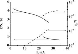
Figure 42. Reduced electric field (solid lines) and ionization degree (dashed lines) at the axis of the discharge tube calculated for argon pressure P = 120 Torr as a function of the discharge current [155].
Download figure:
Standard image High-resolution imageEEDFs in argon at E/N = 3 Td calculated for various ionization degrees by taking into account e–e collisions are shown in figure 43. The set of cross sections for the electron scattering from argon atoms used are the same as in [155]. It is seen that at a low ionization degree the EEDF is strongly non-Maxwellian in the whole energy range and decreases sharply at energies above ∼10 eV. At ne/N > 10−7 a substantial increase in population of high-energy tail of the EEDF is due to e–e collisions (see figure 43).

Figure 43. EEDF in argon at E/N = 3 Td calculated for various ionization degrees by taking into account e–e collisions.
Download figure:
Standard image High-resolution imageAs a result, the rate constants for the excitation of electronic states by electron impact from the ground state also increase with ionization degree. Under the considered discharge conditions, electrons in plasma are produced mainly in stepwise ionization processes. Respectively, the excitation of electronic states by electron impact is the key process for the ionization mechanism. The calculated rate constant for the excitation of the lower metastable state (1s5, in Paschen notation, 11.54 eV) is shown in figure 44 as a function of E/N at various ionization degrees. Figure 44 illustrates that the rate constant strongly grows with the ionization degree at low E/N values. In particular, at E/N = 3 Td the ratio of k(ne/N = 10−6) to k(ne/N = 0) is about one hundred.

Figure 44. Rate constant for the excitation of argon lower metastable state as a function of E/N value calculated for various ionization degrees.
Download figure:
Standard image High-resolution image
8. Conclusions
In the paper an overview is given on effects in non-thermal plasma initiated by deformation of the EEDF. Particular attention is paid to mechanisms of instabilities based on non-linearity of plasma properties for specific conditions: gas composition, steady-state and decaying plasma produced by the electron beam, or by an electric current pulse. The following effects are analyzed: the negative differential electron conductivity; the absolute negative electron mobility; the stepwise changes of plasma properties induced by the EEDF bi-stability; thermo-current instability and the constriction of plasma column in rare gas glow discharge. Mixtures of gases, in which the negative differential conductivity occurs, are potential candidates for using in electron-beam-sustained discharge switches and in gas-filled detectors for radiation detection and dosimetry. As to the absolute negative electron mobility, it was experimentally observed in Xe plasma produced by a short x-ray pulse under low electric field. The absolute negative electron mobility was detected at the stage of EEDF relaxation, as predicted by the theory, and disappeared on a time scale of nano-seconds. The absolute negative electron mobility was predicted theoretically for a number of other physical systems but no experimental confirmation was found. An idea about the possibility of finding EEDF bi-stability effect in plasma of rare gases with R–T minimum was supported by indirect experimental data. Similarly, experimental data on the behavior of electron and vibrational temperatures in afterglow in an Ar : N2 mixture were explained in terms of the EEDF bi-stability. It should be emphasized that the thermo-current instability does not yet have a strict experimental confirmation. The authors hope that this overview will encourage experimenters to reveal the predicted phenomena under theoretically expected conditions. While the constriction of the glow discharge plasma column was comprehensively studied experimentally and has a semi-analytical explanation, the detailed numerical model of this phenomenon was formulated recently. In this paper, we did not include physics of plasma striations observed experimentally in many non-thermal plasma studies. This topic was recently analyzed in detail in an excellent overview by Tsendin [159].