

Abstract
A formula for demagnetizing correction of the measured permeability of cylindrical samples is derived. The procedure for using this formula and the accurately calculated fluxmetric demagnetizing factors to treat the results of fluxmetric measurements is introduced and applied to several samples of different lengths cut from the same magnetic cylinder. The revision of ASTM A342, standard test methods for permeability of feebly magnetic materials, is explained in the appendix.
Export citation and abstract BibTeX RIS
1. Introduction
When an ellipsoid is made of material with constant susceptibility χ and is placed in a uniform applied field Ha along a principal axis, its magnetization M and the demagnetizing field Hd produced by surface poles are both uniform and parallel to Ha. The demagnetizing factor N is defined by Hd = −NM and calculated analytically [1]. This definition of the demagnetizing factor cannot be used for bodies of other shapes, since uniform Ha leads to non-uniform M and/or Hd in general. However, if the volume or midplane averaged M and Hd are both parallel to Ha, a magnetometric or fluxmetric demagnetizing factor may be defined as Nm, f ≡ −〈Hd〉vol, mid/〈M〉vol, mid, where 〈Hd〉vol, mid and 〈M〉vol, mid are the components of volume or midplane averaged Hd and M, respectively, on the Ha axis. Since the volume or midplane averaged field 〈H〉vol, mid = Ha − Nm, f〈M〉vol, mid, χ may be corrected from the measured external susceptibility χext ≡ 〈M〉vol, mid/Ha by

In this work, we study cylinders of length 2Ls and radius Rs, whose Nm, f are functions of the aspect ratio γ ≡ Ls/Rs and χ. To use equation (1), a large number of values of Nm, f over a large range of γ and χ have to be calculated accurately. Before the 1990s, there were complete analytical or accurate numerical calculations of Nm, f only for cylinders of χ → 0 or → ∞ [2–4] and a few accurate but complicated numerical calculations of Nm for χ = −1 and ∞ and γ from 0.25 to 4 [5, 6]. Accurate calculations of Nm, f at many values of γ and χ became possible only when a numerical technique with a vital correction was developed in [7]. After a conjugate relation was studied, optimal data points of χ could be chosen, so that the number of calculated Nm, f points could be greatly minimized and the final results of Nm, f(γ, χ) of accuracy 0.1% are tabulated in [8].
Equation (1) for Nm is relevant to magnetometric measurements, by which the magnetic moment of the entire sample is obtained directly. It has been explained in [8] how to make interpolations from the calculated data points to obtain Nm for any values of γ and χ and how to use equation (1), or more explicitly to use

to obtain χ and Nm iteratively from the directly measured χext and γ. Equation (2) has been compared with experimental data for magnetometric measurements of superconducting and soft magnetic cylinders with the field applied along the axis and a diameter, respectively [9, 10].
Magnetometric measurements are usually carried out for small samples by using instruments such as dc magnetometers and ac susceptometers commercially available. For relatively large samples, fluxmetric measurements are often performed, for which the directly measured quantity is a certain kind of average flux density B but not M so that equation (1) cannot be used. In this work, we develop a formula for the fluxmetric case and use it for demagnetizing correction.
2. Samples and measurements
Cylindrical samples of radius Rs = 0.005 m (cross-sectional area As = πR2s) and different lengths were cut from a high-resistivity iron alloy rod. Low-field ac susceptibility was measured with a lock-in amplifier at f = 40 Hz and at maximum applied field less than 20 A m−1. After a B-measuring coil of number of turns NB = 10 was tightly wound around the midplane with a wire of thickness 0.2 mm, the cylindrical sample was inserted in the center of a solenoid of length LH = 0.392 m, radius 0.0106 m and number of turns NH = 300, whose winding was connected to a resistance R0 = 10 Ω and then to the internal oscillator of a lock-in amplifier, to be magnetized. The voltage across the resistance, VH, and the in-phase and out-of-phase (with respect to VH) voltages across the B-measuring coil, VB1 and VB2, were measured by the lock-in amplifier to obtain the applied field Ha and the cross-sectional out-of-phase and in-phase flux densities, B'' and B', based on the Ampère law and Faraday law, respectively. The in-phase and out-of-phase external permeabilities are calculated by
Since the measured low-field B''/B' at 40 Hz for all samples is smaller than 0.02, the obtained μ'ext is regarded as its dc limit μext.
3. Measuring results and demagnetizing correction
The measured μext for five cylindrical samples of γ between 3.15 and 7.20 is listed in table 1 and shown in figure 1 by open circles. The external permeability is defined, equivalent to equation (3), as μextμ0 ≡ Φ/AsHa, where Φ is the flux through one turn of the B-measuring coil. Since Φ/μ0 = 〈M〉midAs + [Ha − N*f(γ, χ)〈M〉mid]Ac, where Ac is the average area of the coil and N*f is the fluxmetric demagnetizing factor when the midplane average of M and Hd is made within As and Ac, respectively, we have
Using equation (5), equation (1) is written in the fluxmetric case as
N*f(γ, χ) may be replaced by Nf(γ, χ) when Ac is not much larger than As as in the present case, so that equation (6) may be simplified as

The measured μext may be iteratively corrected to χ by using this equation and the calculated Nf(γ, χ).
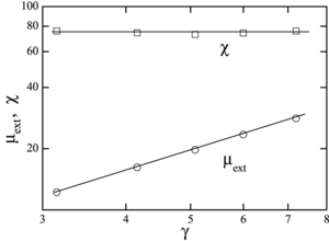
Figure 1. The directly measured external relative permeability μext (circles) and the corrected susceptibility χ (squares) as functions of the aspect ratio γ of five cylindrical samples. Lines are the guide for the eye.
Download figure:
Standard imageTable 1. Measured μext and iterated [Nf(γ, χ(i)), χ(i + 1)] for the studied cylinders.
| γ | μext | i = 1 | 2 | 3 | 4 |
|---|---|---|---|---|---|
| 3.15 | 12.20 | 0.065 27, 55.0 | 0.069 36, 72.8 | 0.069 74, 75.1 | 0.069 78, 75.3 |
| 4.16 | 16.19 | 0.045 34, 57.1 | 0.048 70, 71.8 | 0.049 09, 74.0 | 0.049 14, 74.3 |
| 5.08 | 19.75 | 0.034 31, 58.2 | 0.037 21, 70.7 | 0.037 58, 72.7 | 0.037 63, 73.0 |
| 6.00 | 23.45 | 0.026 90, 60.8 | 0.029 34, 72.0 | 0.029 67, 73.8 | 0.029 72, 74.1 |
| 7.20 | 28.20 | 0.020 55, 64.7 | 0.022 57, 74.8 | 0.022 85, 76.5 | 0.022 89, 76.7 |
The procedure is described in figure 2 for the case of γ = 4.16. Continuous cubic-spline Nf versus γ curves for χ = 1.5, 9, 99 and 999 are plotted in figure 2(a) on log–log scales based on table 1 in [8]. Nf values at γ = 4.16 and χ = 1.5, 9, 99 and 999 are obtained from the crossing points of these curves and the vertical γ = 4.16 line, and the continuous cubic-spline Nf(γ = 4.16, χ) curve is drawn in figure 2(b) on log-linear scales. For iterations, equation (7) is rewritten as

Iteration starts from i = 1 with χ(1) = μext and then increases to i = 2, 3, ... until the difference between χ(i + 1) and χ(i) becomes smaller than 1%. The iterated results for [Nf(γ, χ(i)), χ(i + 1)] are shown by the crossing points between the curve and the vertical lines in figure 2(b) for the case of γ = 4.16. The corrected χ as a function of γ is shown in figure 1 by open squares. We observe that while the measured log μext increases linearly with log γ, the corrected χ becomes constant at χ = 74.7 ± 3%.

Figure 2. (a) The calculated Nf of a cylinder as a function of γ for χ = 1.5, 9, 99 and 999. (b) Nf as a function of χ for a cylinder of γ = 4.16.
Download figure:
Standard imageAs a reference, the interpolated Nf as a function of χ is listed in table 2 and the iterated results of [Nf(γ, χ(i)), χ(i + 1)] are listed in table 1 for all the samples with different values of γ.
Table 2. Values of Nf for the studied cylinders interpolated from the accurately calculated data in table 1 of [8].
| γ | χ = 1.5 | 9 | 99 | 999 |
|---|---|---|---|---|
| 3.15 | 0.052 72 | 0.063 91 | 0.070 08 | 0.070 78 |
| 4.16 | 0.032 85 | 0.042 89 | 0.049 55 | 0.050 35 |
| 5.08 | 0.022 81 | 0.031 37 | 0.038 11 | 0.038 96 |
| 6.00 | 0.016 49 | 0.023 65 | 0.030 20 | 0.031 12 |
| 7.20 | 0.011 47 | 0.017 09 | 0.023 32 | 0.024 28 |
4. Discussion
If Nf is replaced by Nm, equation (7) may also be used for volume-averaged μext when the B-measuring coil uniformly covers the entire length of the cylinder. However, additional error due to possible non-uniformity of the winding has to be considered.
The results here and in [8] are valid for materials with constant χ. For a ferromagnetic cylinder as in the present case, the constant χ is realized at a small applied field, below which χ does not change, and at low frequency, where the eddy-current shielding effect is weak, so that μ''exp/μexp' ≪ 1 and μ'exp is regarded as the initial dc permeability. If μ''exp is not negligible, ac hysteresis has to be considered and equations (2) and (7) should be used for complex ac susceptibility or permeability expressed by χ = χ' − jχ'', χext = χ'ext − jχ''ext and μext = μ'ext − jμ''ext. The problem of demagnetizing correction when considering hysteresis has to be studied for different situations and purposes.
For the ac susceptibility of conducting or superconducting cylinders, where the magnetic moment arises from circulating eddy currents or supercurrents rather than local material χ, Nf, m for χ = −1 should be used with γ > 5 for studying the frequency or field dependence, as shown by direct calculations in [8]. When the frequency dependence of low-field susceptibility of a soft ferromagnetic cylinder is studied, Nf, m for χ equal to dc μext should be used, and γ should be large enough so that 1/Nf, m be comparable with μext and low-frequency demagnetizing correction may be performed with adequate accuracy.
Comparing equation (2) with equation (7), we see that even for an ideal winding with Ac/As = 1, for which equation (7) is exactly valid, χext in equation (2) is replaced by μext − 1 in one place of equation (7) and by μext in another place. This is a consequence of the validity of χext, mid = (μext − 1)/(1 − Nf) rather than χext, mid = μext − 1.
If Ac/As > 1, then N*f < Nf, since the demagnetizing field outside the cylinder is smaller than that inside (see the appendix). In this case, equation (6) should be used. Comparing equation (6) with equation (2), we see an extra term N*f(γ, χ)Ac/As in equation (6). This feature is of great importance in measurements of weakly magnetic samples, for which N*f(γ, χ)Ac/As may be much larger than (μext − Ac/As)Nf(γ, χ) if χ ≪ 1 and Ac/As ≫ 1 (for increasing the measuring sensitivity, a large NB requires the B-measuring coil to be wound multi-layered with a large Ac), so that the demagnetizing correction may be much larger than what is intuitively thought without considering the extra term. This has led to a major revision of the fluxmetric method in an ASTM standard [11], avoiding the error owing to incorrect demagnetizing correction, which could reach 30%. The revision was based on a paper written in Chinese [12], whose main results are reviewed and improved in the appendix.
When χ is large, the above feature of equation (6) becomes less important, and the accurate determination of χ requires sufficiently large γ, as in the situation of equation (2) for the magnetometric case. Although ring samples with circular magnetization (so without demagnetizing effects) are standard for the case of high χ, direct measurements of midplane and volume-averaged μext on a long cylinder to study χ and its uniformity are especially important for certain magnetic devices, such as the magnetic core of a self-inductance or a magnetic torquer rod for spacecraft attitude control [13]. In such devices, large values of material χ are required throughout the entire core or rod and are realized by optimizing material composition and heat treatment. The χ check using the proposed technique may provide important data for quality improvement, which could be vital for a very long torquer rod.
All the above statements for cylinders are basically valid for rectangular prisms, for which the values of Nm, f as functions of aspect ratios and χ are accurately calculated and tabulated in [14]. We note that exact formulas for Nm, f of rectangular prisms at χ → 0 are derived in [15, 16].
5. Conclusion
Demagnetizing correction is used for converting the measured magnetic permeability of a sample with a finite length along the applied field to the intrinsic susceptibility of the sample material. Such a correction may be made straightforwardly when the sample susceptibility is obtained by magnetometric measurements, but extra work has to be done if the directly measured property is permeability. We have derived the correction formula, equation (7), for the latter case, and its applicability for cylindrical samples is shown experimentally. The importance and applications of such a correction are also discussed.
Acknowledgments
This work was financially supported by the National Natural Science Foundation of China (no 61171003), the Beijing Municipal Natural Science Foundation (no 1102024) and the New-Star of Science and Technology supported by Beijing Metropolis (no 2008A020).
Appendix.: Revision to ASTM designation A342
The fluxmetric method in ASTM designation A342, standard test methods for permeability of feebly magnetic materials, originally published as A342-49 and followed till A342-84 was revised to A342-95 in 1995, based on a paper [12] written in Chinese. Some changes made in the revision are explained here for facilitating more readers.
A342-84 signifies the sample cross-sectional area As ⩾ 0.2 cm2, sample length 2Ls ⩾ 10 cm, equivalent dimension ratio of the sample γ ⩾ 4, 20 and 30 for χ < 0.1, 0.1–1 and 1–3, respectively, the length of the test coil Lc ⩽ 2.54 cm and the outer cross-sectional area of the test coil Ac2 ⩽ 10As. Ac2 is allowed to be larger than 10As when χ ⩽ 0.05. The measuring error of χ (written erroneously as permeability μr = 1 + χ) is assigned less than 2%.
Since both the measuring errors of the flux Φ and applied field Ha should be around 1%, only the positive demagnetizing error with respect to the field H,
is considered. It may be estimated by using the accurate values of Nf(γ, χ) for cylinders given in [8] that δh ⩽ 0.29%, 0.13% and 0.19%, for χ < 0.1, 0.1–1 and 1–3, respectively. All these values are negligible compared with the assigned error 2%.
However, A342-84 has ignored a much larger negative demagnetizing error with respect to magnetization M,

Since the test coil is multi-layered, N*f(γ, χ) and Ac are the average of those defined in section 3, considering the total flux of demagnetizing field linked to an NB-turn infinitely short test coil uniformly wound on the midplane with inner and outer radii R1 = α1Rs and R2 = α2Rs, respectively.
For a cylindrical sample of radius Rs and length 2Ls = 2γRs at χ = 0 and a test coil described above, N*f(γ, χ) is calculated by
where
Correspondingly, Ac is calculated by
Nf and N*f at χ = 0 calculated using equations (A.3) and (A.4) as functions of γ are shown in figure 3. We see that N*f < Nf at any given value of γ, and N*f decreases with increasing α2 at fixed γ and α1.
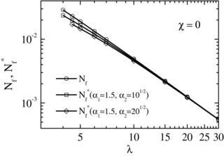
Figure 3. Nf for a cylinder of χ = 0 and the corresponding fluxmetric demagnetizing factor N*f with respect to an infinitely short test coil of relative inner and outer radii (α1, α2) as functions of γ.
Download figure:
Standard imageUsing N*f(γ, χ = 0) shown in figure 3 and assuming N*f(γ, χ)/Nf*(γ, 0) = Nf(γ, χ)/Nf(γ, 0), where Nf(γ, χ) is given in [8], we obtain approximate N*f(γ, χ), so that δm may be calculated using equations (A.2) and (A.5). The results relevant to A342-84 are that −δm ⩽ 13.4–13.7%, 0.70–0.73% and 0.32–0.35% for χ < 0.1, 0.1–1 and 1–3, respectively, when (α1 = 1.5, α2 = 101/2) is used, and if (α1 = 1.5, α2 = 201/2) is used for χ ⩽ 0.05, −δm can reach 20%. In these calculations, the test coil is assumed infinitely short. A larger δm is expected for a coil with finite Lc, so that the maximum error of χ may reach around 30% if Lc/(2Ls) = 0.254 is assumed.
The easiest way to solve this problem is to assign γ > 30 for all materials of χ ⩽ 3 to obtain both negligible δh and δm. However, this is not realistic or economic for materials with very small χ, for which Rs should be large to increase M-measuring sensitivity. We propose two requirements for assigning the standard dimensions of the sample and test coil: (i) δh be negligibly small; (ii) −δm be relatively small and fixed. These requirements may be satisfied by γ = 10, 15 and 30 for χ < 0.5, 0.5–1 and 1–3, respectively. In this case, δh is negligibly small: δh ⩽ 0.26%, 0.24% and 0.19% for χ < 0.5, 0.5–1 and 1–3, respectively. −δm = 2.69–2.85%, 1.28–1.33% and 0.32–0.35% at (α1 = 1.5, α2 = 101/2) for χ < 0.5, 0.5–1 and 1–3, respectively. Since the difference between the lower and upper limits for each χ range is small, one may use their approximate average, −δm = 2.8%, 1.3% and 0.33%, to make demagnetizing correction. After an additional correction with respect to finite coil length, whose experimental procedure is introduced in [12], the error of χ measurements can be less than 2%.
Based on the above calculations, the main changes made in A342-95 are as follows: γ ⩾ 10, 15 and 30 for χ < 0.5, 0.5–1 and 1–3, respectively; Lc/(2Ls) ⩽ 0.2; Ac2/As ⩽ 10 independent of χ. In this case, without mentioning the total error in χ, the largest negative error in χ due to demagnetizing effects is stated as −3% for χ < 0.5.