

Abstract
Planar quantum squeezed (PQS) states, i.e. quantum states which are squeezed in two orthogonal spin components on a plane, have recently attracted attention due to their applications in atomic interferometry and quantum information [1, 2]. In this paper we present an application of the framework described by Puentes et al [3] for planar quantum squeezing via quantum nondemolition (QND) measurement, for the particular case of spin-1/2 systems and nonzero covariance between orthogonal spin components. Our regime, consisting of spin-1/2 entangled planar-squeezed (EPQS) states, is of interest as it can present higher precision for quantum parameter estimation and quantum magnetometry at finite intervals. We show that entangled planar-squeezed states (EPQS) can be used to reconstruct a specific quantum parameter, such as a phase or a magnetic field, within a finite interval with higher precision than PQS states, and without iterative procedures. EPQS is of interest in cases where limited prior knowledge about the specific subinterval location for a phase is available, but it does not require knowledge of the exact phase a priori, as in the case of squeezing on a single spin component.
Export citation and abstract BibTeX RIS
1. Introduction
It is well known that the Heisenberg uncertainty principle for angular momentum determines that the product of uncertainties in two orthogonal components is lower bounded by the mean value of the commutator between two such operators, i.e., ![${\rm{\Delta }}{J}_{i}{\rm{\Delta }}{J}_{j}\geqslant \frac{| \langle [{J}_{i},{J}_{j}]\rangle | }{2}.$](https://content.cld.iop.org/journals/0953-4075/48/24/245301/revision1/jpbaa040dieqn1.gif) For the case of commuting operators, or in the case that the mean value of the third angular momentum component is zero (i.e.,
For the case of commuting operators, or in the case that the mean value of the third angular momentum component is zero (i.e.,  ), the uncertainty relation states that the product of orthogonal variances on a plane should be positive, but there is no limitation on the values that each variance can take separately. In recent years, a type of 'intelligent' [6], quantum spin squeezed state has readily been constructed for the Stokes parameters of light [7–9], and this notion has recently been extended to the collective spin of atomic ensembles [1, 2], for which both variances are equally reduced below the shot-noise level for a coherent state, i.e.
  the so-called planar quantum squeezed state (see figure 1). Such planar squeezed states are defined to satisfy the lower bound on a planar spin variance sum:

where CJ has a fractional exponent behavior dependent on the total spin J [1]. States at this bound have squeezed variances with the same fractional exponent in two components, while increasing the variance in the third component orthogonal to the plane. They are therefore named as planar quantum squeezed states. We note that quantum states which have zero variance in one component, e.g.,  are not suitable candidates for planar quantum squeezing as it is not possible choose a state for which both variances on a plane are equal to zero [2], which sets, in turn, a lower bound on
  He et al [1] provided asymptotic values for the bound CJ, for different values of spin-J. It is remarkable that the lower value of
  corresponds to the case of
  Therefore, the case of spin-1/2 is of particular relevance as it corresponds to the lower bound that can be attained for planar quantum squeezing. This is the limit we analyze in this paper.
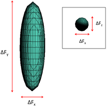
Figure 1. Graphic depiction of generic spin uncertainties  (with
(with  ) in the xy-plane. Only the x-direction has a reduced uncertainty. Inset shows spin uncertainties
  (with
(with  ) on the xz-plane, where planar quantum squeezing takes place as both
  -directions show uncertainty reduction, or squeezing.
Download figure:
Standard image High-resolution imageAs shown in [1–3], planar quantum squeezing (PQS) has the prospect of improving the precision of atomic interferometers at arbitrary phase angles, as it requires both orthogonal variances to be below the shot-noise level and with the same scaling. This is as opposed to squeezing on a single direction, which can only be applied to determine a particular phase angle, known a priori. In addition, PQS states reduce phase noise everywhere on a plane in a single shot, and can therefore be employed in cases where iterative approaches are not applicable. Thus they have promising applications in high-bandwidth atomic magnetometry [10, 11]. In particular, PQS can also be of interest in situations when the phase is not known to a good approximation or when such phase does not remain constant during repeated measurements, as it requires a minimal number of measurements. Such measurement strategies are radically different from those employing multiple sequential measurements, which inherently assume that the phase-shift is a time-invariant, classical parameter.
In [1], the authors proposed the ground state of a two-well BEC Hamiltonian as a paramount example of a planar squeezed state, which saturates the bound of the inequality in equation (1). Interestingly, states presenting maximal PQS have also been proven to display quantum many-body entanglement, satisfying  [1]. In this paper, we propose an extension of the framework for PQS in spin-1 cold atomic ensembles via quantum nondemolition measurements as presented in [3–5] for the case of spin-1/2 systems. For applications in parameter estimation, we focus on the regime of nonzero covariance between orthogonal spin components
  Such PQS states can present macroscopic entanglement, and are therefore referred to as entangled planar quantum squeezed (EPQS) states. The EPQS regime for the case of spin-1/2 systems has not been studied in detail before. This regime is of interest as it can present the largest precision in quantum parameter estimation at finite parameter intervals. Our system presents realistic conditions which can provide PQS and EPQS, with potential applications in high bandwidth atomic magnetometry on a plane, without the need for exact prior phase information.
In our approach, the PQS state is prepared by the stroboscopic probing of a polarized ensemble of cold Rb87 atoms, with the aid of a constant external magnetic field which provides the planar Larmor precession required in order to squeeze two orthogonal components by sequential measurements. In this particular realization, we work with the collective angular momentum variable  for spin-1/2 systems, but we note that this framework has been generalized to higher collective spins numbers [3]. The collective atomic spin is measured using paramagnetic Faraday rotation with an off-resonant probe. The ensemble of spins, polarized along a fixed direction by optical pumping, interacts with an optical pulse of duration τ and polarization described by the Stokes vector
  through an effective Hamiltonian Heff.
The article is structured as follows. In section 2, we briefly review the formalism for light-matter interaction in spin-1/2 systems. Next, in section 3, we present numerical evidence of PQS in the spin-1/2 system, and we detail the connections between planar squeezing, entanglement and optical depth. In section 4, we provide an example for the application of these ideas in high bandwidth atomic magnetometry for entangled planar quantum squeezed (EPQS) states, corresponding to the case of nonvanishing covariance between orthogonal spin components. Finally, in section 5 we present our conclusions.
2. Light–atom interaction
The formal description of this ultra-sensitive measurement is complicated and has only recently been formulated considering the magnetic field, the atoms and the light as one large quantum object. This description allows us to estimate the expectation values and the uncertainty of the quantity of interest, as described in [3, 4], for spin-1 systems.
2.1. Continuous variables for light and atoms
Polarized light in continuous variables can be described with Stokes operators (taking  ) [14–16]:

where  and
and  are the annihilation operators for the left and right circular polarization and

 the Pauli matrices. The
 and
and  Stokes operators represent, respectively, linearly polarized light horizontally or vertically, linearly polarized light in the
  direction, and right-hand side or left-hand side circularly polarized light, respectively. They have the same commutation relations as angular momentum operators. We will work with highly polarized states. For example, for horizontally polarized light pulses we have:

where Nph is the number of photons. The variances are then defined as:

Similarly, for an ensemble of spin-j atoms we can define collective angular momentum operators states in terms of the single-atom angular momentum operators  in the form:

where we have assumed symmetry under particle exchange, and total number of atoms NA. The collective atomic spin operators  here defined allow us to characterize macroscopically the dynamics of the atomic ensemble.
2.2. Atom–light interaction in an external B-field
The effective Hamiltonian describing the interaction of a homogeneous system of  spins, interacting with off-resonant light, up to an overall constant has the form [17]:

where  are the vector (tensor) components of the polarizability that depend on the atomic absorption cross section, the beam geometry, the detuning from resonance Δ and the hyperfine structure of the atom. Here μ is a coupling constant,
  and
and  stand for the collective spin and magnetic field, respectively. Note that the Hamiltonian analyzed in the paper is not equivalent to the one studied previously in [3], which further motivates our numerical exploration. Here we are ignoring contributions from the tensorial light shift
  We performed numerical simulations that confirm that the addition of this term does not modify the dynamics.
The coherent evolution of a phase-space vector v, describing the state of the whole system [4, 14, 16], for a time duration τ, described by the Hamiltonian Heff, is given to first order in τ by:

where the matrix  determines the linear evolution of v(t) during the time interval τ. The linearity of (7) is a consequence of the linear Hamiltonian in (6). The second moments and variances of the phase-space vector v are conveyed in the covariance matrix [14, 17].
The strategy to generate planar squeezing can be described as follows: an initial state is prepared and forced to precess in the x–z plane by an external magnetic field oriented along y ( term in
  ). Short pulses of light, on the time scale of the precession, initially polarized along Sx, are sent through the ensemble at quarter-cycle intervals. Through the
  term, the light–atom interaction rotates the polarization from Sx toward Sy by an angle proportional to
  A measurement of Sy then gives an indirect measurement of Jz, reducing its uncertainty (
 ) with minimal back action. It is therefore referred to as quantum nondemolition (QND) measurement. If this measurement is sufficiently precise it squeezes the uncertainty in Jz. A quarter cycle later, the state has precessed so that the Jx component can be measured, and possibly squeezed. The coupling effect of the tensorial G2 term can be exactly suppressed by dynamical decoupling, as described in [17].
While a given spin component can be squeezed by QND measurement, it is in principle not obvious that planar squeezing, which requires simultaneous squeezing of noncommuting observables, should be producible by the same mechanism. Nevertheless, if  the angular momentum Heisenberg uncertainty relation does not impose measurement back-action on Jx when Jz is measured, nor vice versa. This suggests that sequentially measuring Jx and Jz should squeeze both spin components and thus give planar squeezing.
3. Numerical results
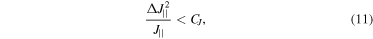
In this section, we present numerical results validating the use of QND measurement in cold atomic ensembles for conditional preparation of planar quantum squeezed states [3], for the case of spin-1/2 systems. We stress that obtaining numerical results for the case  is of particular interest as it can provide the lowest bound on planar quantum squeezing
  The operational definition we adopt for planar quantum squeezing follows the approach by He et al [1, 2], and can be summarized as follows. First, from equation (1) and permutations, we take
  as the standard quantum limit (SQL) [18], where
  is the magnitude of the in-plane spin components. We define the planar variance
  with SQL
  and the planar squeezing parameter

We performed numerical simulations for stroboscopic probing [3, 12], in a cold atomic ensemble containing  87Rb atoms with coupling parameter
  corresponding to a detuning in the off-resonant probe given by
  The atomic ensemble is initially polarized in the x-direction by optical pumping and prepared in the state
  with 99.9% fidelity, and technical noise due to atom number fluctuations given by
  The initial collective atomic spin mean values are
 and
and  Additionally, we introduced an external magnetic field
  mG, which sets a Larmor precession in the (
 )-plane, with a characteristic period of
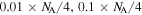
  μs. We chose this magnitude for By in order to allow sufficient time within a Larmor cycle for stroboscopic probing. The atomic ensemble is probed at four instances during the Larmor cycle by a single off-resonant optical pulse at each location. The atomic cloud is left free to precess at time intervals given by
  in order to probe the collective atomic spin sequentially on a plane (
 ), as required for planar quantum squeezing. The length of optical pulses in the sequences is τ = 1 μs, and each pulse contains
  photons. The optimal number of photons on each individual pulse was obtained as a trade-off between maximal squeezing and minimum loss of atomic polarization due to optical scattering.
Numerical simulations confirming PQS for spin-1/2 are
shown in figures 2–4. The ensemble of atoms is initially polarized in the x-direction, and precesses in the ( )-plane due to the B-field at the Larmor frequency. Mean values of collective atomic spins are displayed in figure 2. We evaluated the normalized variances on the plane for the collective angular spin components after sequential stroboscopic probing on a plane (figure 3
). The individual normalized variances on the (
)-plane due to the B-field at the Larmor frequency. Mean values of collective atomic spins are displayed in figure 2. We evaluated the normalized variances on the plane for the collective angular spin components after sequential stroboscopic probing on a plane (figure 3
). The individual normalized variances on the ( )-plane oscillate as a consequence of the Larmor precession, and are sequentially reduced due to the stroboscopic probing, as indicated by the discontinuous jumps in
  (red curve). On the other hand, the uncertainty in the orthogonal direction
  is sequentially increased well above the SQL (dashed line), as expected for a planar quantum squeezed (PQS) state. The ideal planar quantum squeezed state, for the system parameters chosen, is achieved at approximately 300 μs. Figure 4 shows the planar squeezing parameter
  for spin-1/2 systems. It is seen that for short times this parameter is below the unity SQL (dashed line), and is sequentially reduced to less than
  with each individual components squeezed to
  , which confirms the presence of planar quantum squeezing in the system. The inset in figure 4 shows a reduction by 40% in the normalization factor
  due to optical scattering during the probing sequence, which in turns limits the maximal planar squeezing that can be obtained.

Figure 2. Mean values of collective atomic angular momenta for spin-1/2 systems. Gray curve  black curve
  and red curve
  The mean value in the direction orthogonal to the plane of precession remains always approximately zero
  as required for planar quantum squeezing.
Download figure:
Standard image High-resolution image
Figure 3. Normalized variance of collective atomic spins in spin-1/2 systems. Gray curve  black curve
  and red curve
  At all times the uncertainties on the (x,z)-plane are below the standard quantum limit (SQL = 1) indicated by the dashed line, and are decreased at the expense of increasing noise in the orthogonal direction (red curve). The discontinuities in
  correspond to probing events. Maximal planar quantum squeezing is achieved at approximately 300 μs.
Download figure:
Standard image High-resolution image
Figure 4. Planar squeezing parameter  for spin-1/2 systems. For sufficiently short times the planar uncertainty remains below the standard quantum limit (SQL = 1), as indicated by the dashed line, and can be reduced sequentially due to stroboscopic probing. Maximal planar quantum squeezing is achieved at approximately 300 μs and is reduced at longer times due to loss of atomic polarization by optical scattering. Inset shows the normalization factor
  which is reduced by 40
  due to optical scattering during the total measurement time.
Download figure:
Standard image High-resolution image3.1. Limits on planar quantum squeezing due to optical scattering
In the absence of optical scattering and spontaneous emission the squeezing that can be obtained by QND measurements is of the order  where
where  is the scalar atom–light coupling parameter. The quantum uncertainty after squeezing can be expressed as
  where
where  is the nominal uncertainty for a coherent state in a spin-1 system. This would suggest that infinite squeezing can in principle be achieved by increasing κ. However, there are severe limitations on the amount of squeezing that can be achieved due to spontaneous emission. In fact, the coupling parameter κ can also be expressed as
  where α is the atomic ensemble optical column density, and
  is the spontaneous emission rate. A basic estimate for the squeezing parameter in the presence of optical scattering can be expressed by
  and it is minimum for an optimal spontaneous decay probability
  For a typical system with optical density
  this optimal value gives a lower bound on the amount of squeezing given by roughly
  (3 dB of noise reduction) [19].
A similar argument can be employed to determine a lower bound on the squeezing parameter that can be achieved for planar quantum squeezing via QND measurements. Following the definition of  we can define a similar expression for the planar squeezing parameter
  in terms of the individual squeezing parameters
  in the following form:

where  and
and  Assuming the same optical depth in both directions
  we can estimate the minimum planar squeezing parameter to be
  (roughly 2 dB of noise reduction). This is depicted in figure 4, for experimentally feasible values for the optical depths
  where the red line indicates the quantum limit.

Figure 5. Minimal planar squeezing parameter  in terms of optical depth (α) for spin-1/2 systems. α should be above 10 in order to achieve a planar squeezing parameter below the standard quantum limit (SQL)
  , indicated by the red line.
Download figure:
Standard image High-resolution image3.2. Planar squeezing and entanglement criteria for spin-1/2 systems
Quantum entanglement represents a resource for most quantum information protocols, as well as a key ingredient for atomic and optical interferometric schemes, allowing for the reduction of noise below the standard quantum limit (SQL), and providing maximal sensitivity in fundamental quantum metrology applications. Despite its relevance, the verification of entanglement in many-body systems is a remarkably challenging task. For the case of atomic ensembles of spin-1/2 particles there exist clear entanglement criteria involving spin squeezing inequalities. The criteria for bipartite entanglement for qubits (i.e., spin-1/2) results in [13]:

where  is the projection of the total spin
  in the direction
  A plot of the LHS of the inequality
  and the RHS of the inequality (
 ) are shown in figures 6 and 7, respectively, for time intervals of 1000 μs. The difference between these two magnitudes is shown in figure 8. It is observed that the difference is always positive, therefore with this definition of the spin squeezing parameter
  there is no observable bipartite entanglement. The reason for this is that the normalization in equation (eq:10) includes the y-direction where there is clearly no entanglement at all, since
  for all times (see figure 2).

Figure 6. Plot of spin squeezing parameter  with (
 ).
).
Download figure:
Standard image High-resolution image
Figure 7. Plot of normalized spin mean values  with (
 ) versus time between 0 μs and 1000 μs.
Download figure:
Standard image High-resolution image
Figure 8. Entanglement criteria based on spin inequality (equation (10)). The quantity  with (
 ) is always positive, thus revealing no observable entanglement based on this entanglement criteria.
Download figure:
Standard image High-resolution imageMore recently, in [1], the authors derived a simple inequality able to detect nonclassical behavior in a mesoscopic system consisting of a large number spins J. The general form of the entanglement criteria involves two variances on a plane, and is particularly suitable for the characterizations of quantum entanglement in PQS states, thus providing a tight bound for the entanglement content. The entanglement condition can be expressed as:
For the case of spin-1/2 systems the asymptotic limit for this expression becomes  [1]. We note that the limit CJ reaches a minimum for spin
  and for this reason spin-1/2 systems are of particular interest for metrological applications as they can provide the lowest precision bound, which motivates the numerical calculations presented in this paper. The amount of planar squeezing that can be achieved in our system, as quantified by the normalized planar variance
  versus the optical depth (α), is plotted in figure 9. In order to beat the classical bound
  an optical depth above
  is required. Even though in our system
  does not reach the
  bound (see figure 4 for reference), we note by considering higher optical depths this bound can, in principle, be achieved in current experimental configurations [3]. This entangled regime is analyzed in the following section in the context of atomic interferometers and quantum magnetometry.

Figure 9. Planar squeezing parameter versus optical depth (OD) for spin-1/2 systems. The classical limit (red line) is indicated by the asymptotic value  [1]. For
  it is possible to observe mesoscopic entanglement in the system.
Download figure:
Standard image High-resolution image4. Applications: atomic interferometers and quantum magnetometry
Experimentally determined phase shifts are never truly classical, nor time invariant [2]. Phases always vary within some timescale, and cannot always avoid measurement back action, a limitation that can rule out the possibility of iterative techniques. The physical reason for this is that phase shifts are related to energy shifts terms in the radiation field Hamiltonian [20]. In fact, the problem of defining a Hermitian quantum phase operator  dates back to the early attempts by Dirac [21]. It has been demonstrated that for the case of a bosonic mode
  a Hermitian operator
  satisfying
 ![$[\hat{{\phi }_{a}},\hat{{N}_{a}}]=-i,$](https://content.cld.iop.org/journals/0953-4075/48/24/245301/revision1/jpbaa040dieqn124.gif) where
where  is the number of bosonic particles in the mode, does not exist [22]. Hermiticity is at the core of this limitation and can also be considered at the core of the quantum phase-estimation problem. Nevertheless, upon some approximations, such as large particle number, canonical commutation relations for the phase operator do exist, and lead to a fundamental uncertainty principle, i.e. the Heisenberg limit:

The pioneering work by Caves [24], showed that in order to beat the standard quantum limit (SQL), or shot-noise limit of  a phase-squeezed input state is required, reaching maximum sensitivity at the Heisenberg limit
  Nevertheless, the treatment of Caves et al [24, 25] also assumed prior knowledge on the phase to be estimated which, in turn, allowed for a linearized treatment, in the limit of small fluctuations. In this paper we consider phase estimation with no prior information, or with only limited prior information using planar quantum squeezed states.
First we describe a particular application of planar quantum squeezing (PQS) in atomic magnetometry, for determination of arbitrary quantum phase parameters below the SQL, without the need for prior information or linearized fluctuations for spin-1/2. PQS states can be used to determine an almost arbitrary phase angle ϕ, within a finite interval along the precession of the collective atomic magnetic moment J. The precession of this vector is determined by a phase  where
where  is the Larmor frequency, which in turn is proportional to the external magnetic field Bext applied on the system, so a high precision in the estimation of parameter ϕ can be mapped onto precision magnetometry. For an external field along the
  direction By, we expect a precession of the collective atomic spin on the
  plane. The rotation of the collective spin on the plane can be written as:

We can calculate the parameter uncertainty via  By differentiating
  we obtain:

where 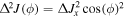

![$+[\mathrm{cov}({J}_{x},{J}_{z})+\mathrm{cov}({J}_{z},{J}_{x})]$](https://content.cld.iop.org/journals/0953-4075/48/24/245301/revision1/jpbaa040dieqn134c.gif)
 Here
Here  stands for the covariance of the operators, given by
For the case  we can write
  We can now set a bound on
  in terms of planar squeezing such that:

therefore obtaining a bound to the quantum noise present in the magnetometer given by the planar variance  which is independent of ϕ, thus confirming that PQS states are optimal for quantum-phase estimation at arbitrary angles. We note that planar quantum squeezed states give the lowest planar variance for any angle, with the exception of the specific singular ones which make the denominator in equation (14) equal to zero. This feature is depicted in figures 10 and 11.

Figure 10. Normalized parameter variance ( ) employing an ideal PQS state. Different curves correspond to different amounts of planar squeezing. The SQL (
 ) is indicated by the gray dashed line. Black, blue, red, magenta, and green curves correspond to atom number variances
 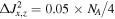 ,
,  ,
,  Sensitivity below the standard quantum limit can be achieved for a broad interval of ϕ parameter values, with the exception of the insensitive regime for singular values in equation (14).
Download figure:
Standard image High-resolution image
Figure 11. Normalized parameter variance ( ) employing an ideal squeezed state on a single spin component. Different curves correspond to different amounts of single-component squeezing. The SQL (
 ) is indicated by the gray dashed line. Black, blue, red, magenta, and green curves correspond to atom number variances
  ,
,  ,
,  while
while  Sensitivity below the standard quantum limit can be achieved only for a few particular values of ϕ, which should be known a priori.
Download figure:
Standard image High-resolution imageFigure 10 shows the normalized phase parameter variance  for an ideal PQS state. Different curves correspond to different levels of planar quantum squeezing. The SQL is indicated by the dashed line. It is clear that PQS states can provide for precision below the SQL for a broad (flat) range of phases. On the other hand, in figure 11 we show the phase parameter variance
  for an ideal squeezing state on a single component. In this case, precision below the SQL (dashed line) can only be achieve for particular phases, which should be known a priori.
4.1. Atomic magnetometry with entangled planar-squeezed (EPQS) states
In this section we consider the interesting regime of nonzero covariances  where the covariance is given by
  The covariance is limited by the individual variances of each operator (
 ). For perfectly correlated operators we obtain
  Such correlations between spin components can arise in the presence of entanglement in macroscopic ensembles [23]. This entangled regime can be achieved in cold atomic ensembles when considering a sufficiently large optical depth (
 ) for the case of spin-1/2 systems, as described in detail in the previous section. The entangled regime is of interest for parameter estimation at specific subintervals in the phase parameter ϕ, which minimize the spin variance, given by:

In particular, for intervals where  states with nonzero covariance
  can reduce the total spin variance
  even below the PQS limit
  and therefore provide higher precision than PQS states. This comes at the cost of some prior knowledge in relation to the actual interval where the phase is located.
The precision enhancement for states with nonzero covariance is displayed in figure 12. Gray curve corresponds to the PQS bound  the black curve corresponds to the balanced case
  and maximal correlation
  the red curve corresponds to the unbalanced case
  and maximal correlation
  The black curve shows that for the phase intervals
 ![$\phi \in [-\pi 2,0]{\rm{U}}[\pi /2,\pi ]$](https://content.cld.iop.org/journals/0953-4075/48/24/245301/revision1/jpbaa040dieqn164.gif) where
where 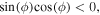 it is possible to surpass the PQS precision limit, for the case
  but for a reduced interval of phase values, therefore requiring some degree of prior information, as opposed to the case of PQS states with no entanglement, which can be used to estimate any arbitrary phase, with no prior knowledge. Such conditions for nonzero covariance can be reached in entangled planar quantum squeezed states (EPQS). For the case of asymmetric (imbalanced) spin components (red curve) the maximal precision is reduced with respect to the balanced case, but it is enhanced in some specific phase ranges with respect to the balanced case (red curve below black curve). In this particular imbalanced case, the precision is enhanced in the subinterval
 ![$\phi \in [-0.75,0].$](https://content.cld.iop.org/journals/0953-4075/48/24/245301/revision1/jpbaa040dieqn167.gif) This imbalance strategy can be used to enhanced precision at specific phase values, with some prior information. Note that this strategy does not require knowledge of the exact phase, as is the case for squeezing on a single component.
This imbalance strategy can be used to enhanced precision at specific phase values, with some prior information. Note that this strategy does not require knowledge of the exact phase, as is the case for squeezing on a single component.

Figure 12. Spin variance  versus phase ϕ, for states with nonzero covariance and maximum correlation
  Such states correspond to entangled planar quantum squeezing (EPQS). The gray curve corresponds to PQS limit
  with zero covariance, the black curve corresponds to the symmetric case
 red curve corresponds to asymmetric case
 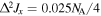 ,
,  with maximal correlation
  It is apparent that the spin variance can be reduced in the intervals
 ![$\phi \in [-\pi /2,0]{\rm{U}}[\pi /2,\pi ],$](https://content.cld.iop.org/journals/0953-4075/48/24/245301/revision1/jpbaa040dieqn175.gif) as expected for
as expected for 
Download figure:
Standard image High-resolution imageFigure 13 displays the quantum parameter variance for EPQS state, for the symmetric case  and
and  Different curves correspond to covariance values ranging between
  As expected in this situation it is possible to achieve higher sensitivities (
 ) than with a PQS state (figure 10) for a broad parameter interval
 ![$\phi \in [-\pi /2,0],$](https://content.cld.iop.org/journals/0953-4075/48/24/245301/revision1/jpbaa040dieqn181.gif) thus confirming that entangled planar squeezed (EPQS) states can be optimal for quantum parameter estimation, at specific (i.e., known) finite intervals. In particular, EPQS states can in principle achieve the Heisenberg limit
thus confirming that entangled planar squeezed (EPQS) states can be optimal for quantum parameter estimation, at specific (i.e., known) finite intervals. In particular, EPQS states can in principle achieve the Heisenberg limit  for states with maximal covariance. Similar results can be obtained for other intervals where
  Figure 14 displays quantum parameter variance for the EPQS state, for the asymmetric case
  and
and  and
and  Different curves correspond to covariance values ranging between

Figure 13. Normalized parameter variance ( ) employing an ideal entangled planar quantum squeezed (EPQS) state with
  The parameter variance is well below the SQL (
 ), and can in principle reach the Heisenberg limit (
 ) for states of maximal covariance. Black, blue, red, magenta, and green curves correspond to atom number covariances
 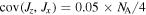 ,
,  ,
,  while
while  Sensitivity well below the standard quantum limit can be achieved for a broad range of parameter values
 ![$\phi \in [-\pi /2,0],$](https://content.cld.iop.org/journals/0953-4075/48/24/245301/revision1/jpbaa040dieqn194.gif) thus confirming that EPQS are optimal for quantum parameter estimation at finite intervals.
thus confirming that EPQS are optimal for quantum parameter estimation at finite intervals.
Download figure:
Standard image High-resolution image
Figure 14. Normalized parameter variance ( ) employing an ideal entangled planar quantum squeezed (EPQS) state with maximal covariance (
 ), for the imbalanced or asymmetric case
  Different curves correspond to different covariances. The parameter variance is well below the SQL (
 ), and can in principle reach the Heisenberg limit (
 ) for states of maximal covariance. Black, blue, red, magenta, and green curves correspond to atom number covariances
  ,
,  ,
,  ,
,  while
while  Sensitivity well below the standard quantum limit can be achieved for a broad range of parameter values
 ![$\phi \in [-\pi /2,0].$](https://content.cld.iop.org/journals/0953-4075/48/24/245301/revision1/jpbaa040dieqn202.gif) Moreover, in the interval
Moreover, in the interval ![$\phi \in [-0.5,0]$](https://content.cld.iop.org/journals/0953-4075/48/24/245301/revision1/jpbaa040dieqn203.gif) the imbalanced case can render higher precision than the balanced case.
the imbalanced case can render higher precision than the balanced case.
Download figure:
Standard image High-resolution image
5. Conclusions
To conclude, by means of a numerical framework extensively described by Puentes et al [3], we have demonstrated that a kind of planar quantum squeezed (PQS) state, which squeezes the variances on two orthogonal spin components, can be prepared in spin-1/2 cold atomic ensembles, via quantum nondemolition (QND) measurements. Such PQS states have important applications in the determination of arbitrary quantum phases below the standard quantum limit (SQL), in a single shot, and are therefore promising candidates for high-bandwidth atomic magnetometry in cases where iterative approaches are not applicable due to dynamical fluctuations. We show the PQS states prepared via QND measurements in spin-1/2 can present many-body entanglement for sufficiently high optical depth and can therefore be optimal, in the sense of saturating the bound in equation (1) [1], for quantum parameter estimation below the SQL with no a priori information. Moreover, we show that for quantum parameter estimation at specific intervals known a priori, entangled planar quantum-squeezed states (EPQS), displaying nonzero covariance between orthogonal spin components, can provide even higher precision that PQS states, turning them into ideal quantum resources for parameter estimation at finite intervals. As a future step, we plan to investigate the effect of losses in the precision control at finite time intervals, and characterize the behaviour of collective spin-1/2 systems in the nonideal scenario [26].
Acknowledgments
The author acknowledges G Colangelo, R Sewell, and M Mitchell for related discussions. GP gratefully acknowledges financial support from the PICT2014–1543 grant and the Raices programme.