

Abstract
The unique dose deposition of proton beams generates a distinctive thermoacoustic (protoacoustic) signal, which can be used to calculate the proton range. To identify the expected protoacoustic amplitude, frequency, and arrival time for different proton pulse characteristics encountered at hospital-based proton sources, the protoacoustic pressure emissions generated by 150 MeV, pencil-beam proton pulses were simulated in a homogeneous water medium. Proton pulses with Gaussian widths ranging up to 200 μs were considered. The protoacoustic amplitude, frequency, and time-of-flight (TOF) range accuracy were assessed. For TOF calculations, the acoustic pulse arrival time was determined based on multiple features of the wave.
Based on the simulations, Gaussian proton pulses can be categorized as Dirac-delta-function-like (FWHM < 4 μs) and longer. For the δ-function-like irradiation, the protoacoustic spectrum peaks at 44.5 kHz and the systematic error in determining the Bragg peak range is <2.6 mm. For longer proton pulses, the spectrum shifts to lower frequencies, and the range calculation systematic error increases (⩽23 mm for FWHM of 56 μs). By mapping the protoacoustic peak arrival time to range with simulations, the residual error can be reduced. Using a proton pulse with FWHM = 2 μs results in a maximum signal-to-noise ratio per total dose. Simulations predict that a 300 nA, 150 MeV, FWHM = 4 μs Gaussian proton pulse (8.0 × 10⁶ protons, 3.1 cGy dose at the Bragg peak) will generate a 146 mPa pressure wave at 5 cm beyond the Bragg peak.
There is an angle dependent systematic error in the protoacoustic TOF range calculations. Placing detectors along the proton beam axis and beyond the Bragg peak minimizes this error. For clinical proton beams, protoacoustic detectors should be sensitive to <400 kHz (for −20 dB). Hospital-based synchrocyclotrons and cyclotrons are promising sources of proton pulses for generating clinically measurable protoacoustic emissions.
Export citation and abstract BibTeX RIS
1. Introduction
Protons have a unique energy deposition that culminates in the Bragg peak (BP). Due to the limited range, proton therapy is theoretically advantageous compared to photon therapy because the proton BP allows for targeted cancer treatment in which organs beyond the target are spared. Based on the sparing potential, radiation oncology departments are investing in proton therapy centers and the number of patients treated with protons is increasing exponentially (Bortfeld and Jeraj 2011). Unfortunately, uncertainty in the proton range limits the benefits of proton therapy. To reduce the risk of over- or under-shooting the tumor, large margins are added and the arrangement of beams is limited so that organs-at-risk are not placed distal to the calculated Bragg peak volume (Knopf and Lomax 2013).
The proton's unique dose deposition profile also generates a unique thermoacoustic wave emission pattern. In thermoacoustic phenomena, energy pulses heat the irradiated medium, expansion occurs in response to the heating, and a longitudinal pressure wave is emitted. The amplitude of the pressure wave is related to the first derivative of the energy pulse. Doubling the number of particles (e.g. photons or protons) in a given pulse will double the resulting emitted pressure amplitude, but changing the temporal characteristics will also affect the pressure magnitude. For photons, in thermoacoustic or photoacoustic imaging, the electromagnetic waves are exponentially attenuated as they penetrate a homogeneous medium. For imaging, the photons bathe the medium with illumination that monotonically decreases with depth. On top of this backdrop, heterogeneous structures are identified based on their higher (or lower) relative absorption, which causes increased heating and the emission of distinguishable, higher-amplitude pressure waves. In contrast to photoacoustics, the unique dose deposited by pencil-beam proton radiation (protoacoustics) creates two macroscopic pressure waves in a homogeneous medium: the pre-Bragg peak volume emits a cylindrical wave that propagates lateral to the proton beam direction (referred to as the α wave) while the Bragg peak emits an approximately spherical wave (the γ wave) (Albul et al 2004, Jones et al 2014). In a heterogeneous medium, the proton beam will act like a spotlight that preferentially illuminates structures within the Bragg peak volume.
Protoacoustics has been suggested as a technique for in vivo proton range verification (Polf and Parodi 2015), and the signal has been measured previously using readily available hydrophones, amplifiers, and oscilloscopes (Sulak et al 1979, Hayakawa et al 1988, Albul et al 2001, Capone and De Bonis 2006, Assmann et al 2015, Jones et al 2015). In theory, by measuring the thermoacoustic emissions generated by the proton heat deposition, the dose deposition can be reconstructed. Schemes to extract information from the protoacoustic signal vary in complexity. With an array of detectors appropriately placed, the 3D dose deposition may be calculated (Alsanea et al 2015). Here, we focus on assessing the potential of determining the Bragg peak position (ie proton range verification) based on the time-of-flight (TOF) of the protoacoustic wave generated by the Bragg peak from a pencil beam scanning (PBS) proton beam. The investigated PBS beam has a spot size large enough that lateral equilibrium is achieved, and a clear Bragg peak is observed. If lateral equilibrium is not achieved (the spot is small), lateral spread can greatly reduce the relative intensity at the Bragg peak.
Although others have previously suggested and used the protoacoustic TOF to estimate the Bragg peak position (Hayakawa et al 1988, Hayakawa et al 1989, Tada et al 1991, Hayakawa et al 1995, Assmann et al 2015), theoretical and/or experimental justification is lacking. Previous studies have postulated that the TOF correlates to the Bragg peak position, but studies assessing this hypothesis have not been performed. For a point pressure source, this assumption is correct, and the acoustic wave arrival time can be used to exactly calculate the distance from the detector. For a spatially asymmetric pressure source, however, the emitted pressure wave will encode the asymmetry of its origin, which may skew the arrival time. We hypothesize that the protoacoustic pressure wave arrival time will be offset from the expected arrival time (given by the distance to the BP divided by the speed of sound) because of the asymmetric nature of the proton dose deposition.
Another under-addressed facet of protoacoustics is the disconnect between the proton pulses used in research experiments and the clinic. Most notably, because the protoacoustic signal is proportional to the first time derivative of the heating rate, we hypothesize that the protoacoustic amplitude will depend on the temporal characteristics of the irradiating proton pulse (Jones et al 2014). Although the protoacoustic amplitude generated by a given proton pulse shape is proportional to the number of protons within the pulse, the amplitude also strongly depends on the shape of the proton pulse. Therefore, pulses depositing equivalent doses (containing the same number of protons) can result in very different protoacoustic signals and amplitudes depending on the pulse's temporal shape. Similarly, aside from affecting amplitude, it is common knowledge in the ultrasound and thermoacoustic fields that the frequency and resolution of acoustic signals depend on the temporal characteristics of their excitation; to improve resolution, high frequency (>1 MHz), short pulses are used in ultrasound and short laser pulses (<100 ns) are used in photoacoustics. In thermoacoustics, the excitation pulse fulfils the condition of stress confinement if it has a pulse-width shorter than the transit time of sound across the irradiated volume of interest (Xu and Wang 2006). If the excitation pulse is longer, then stress confinement is not achieved, and the resulting emitted thermoacoustic pressure waves will be broadened and blurred. With few exceptions, when the rise times were not reported (Sulak et al 1979, Graf et al 2006), previous measurements of the protoacoustic signal have employed short proton pulses (<70 ns) with concomitantly fast rise times (Sulak et al 1979, Hayakawa et al 1988, 1989, Tada et al 1991, Hayakawa et al 1995, Albul et al 2001, 2005, 2004, Capone and De Bonis 2006, Terunuma et al 2007, De Bonis 2009, Bychkov et al 2010, Assmann et al 2015). Clinical proton sources routinely output proton pulses with rise times orders of magnitude longer (Cyclotron: 50 μs (Measurements 2007) and 18 μs (Jones et al 2015), Synchrotron: 200 μs (Measurements 2007), Synchrocyclotron: 7 μs (Kleeven et al 2013)). To become clinically implemented, the manifestation of different proton pulse characteristics on the protoacoustic signal must be understood.
For TOF measurements, researchers are confronted with the question of how to measure the arrival time of a bipolar acoustic pulse, which has multiple measurable features, each of which returns a different arrival time. For example, in ultrasound, the arrival time may be measured at the first arrival time, the center of gravity, or at some threshold pressure level. For this protoacoustic simulation study, four arrival time metrics are compared: the arrival time of the positive compression peak (positive pressure portion of the longitudinal pressure wave), the arrival time of the negative rarefaction peak (negative pressure portion of the longitudinal pressure wave), their average, and the time in between when the pressure crosses from positive to negative. Because different metrics can return arrival times that differ by 10 s of microseconds, it is important to understand the origin and manifestation of using each metric.
The goal of this manuscript is to identify the expected protoacoustic amplitude, frequency, and TOF-based calculation accuracy and to determine their dependence on proton pulse characteristics. The paper is organized as follows. First, the underlying thermoacoustic equations are described and interpreted to trace the origin of the identified trends. Second, the amplitude of the protoacoustic signal is considered with particular focus on the proton pulse dependence, the distance dependence, and the signal-to-noise ratio. Third, the protoacoustic frequency spectrum is described. Next, the accuracy of the TOF range calculation is assessed. Lastly, different arrival time metrics are compared. Overall, the manifestations of using proton pulses with different rise times are determined, and an ideal proton pulse is identified. These simulations represent a necessary step towards assessing the viability of using protoacoustics as a range verification method in the clinic.
2. Methods
2.1. Underlying thermoacoustics
In thermoacoustics, energy pulses cause pulsed heating, which creates expansion that emits longitudinal pressure waves. In the simplest conceptual case, an excited point source will emit a pressure wave proportional to the first time derivative of the excitation pulse. Thus, a Gaussian excitation pulse results in a bipolar acoustic emission consisting of a positive compression (increased pressure) peak—from the increase in the rate of heating as the excitation pulse rises—followed by a negative rarefaction (decreased pressure) peak—from the decrease in heating rate as the excitation pulse falls. The positive and negative pressure peaks are not due to heating and cooling. Rather, they are due to changes in the rate of heating: as the heating rate increases, there is a local expansion and positive emitted pressure, while during decreased heating contraction occurs and a negative pressure wave is observed. Conceptually, extrapolating beyond the point source, the pressure emitted from a complicated energy deposition is the sum of the individual responses that would be observed from decomposing the spatial deposition into point sources. Interestingly, because the acoustic emission depends on the excitation pulse time derivative, the acoustic wave amplitude will depend both on the deposited energy and the temporal shape of the excitation pulse. For a given excitation pulse shape, the thermoacoustic emission amplitude will be linear in the deposited energy (or number of protons for proton irradiation). But, if the excitation pulse has a small first derivative, a large amount of energy can be deposited without generating much thermoacoustic emission. For example, a long rectangular excitation pulse will deposit a large amount of cumulative energy, but acoustic emission will only be generated at the beginning rise (positive, compression acoustic peak) and the ending fall (negative, rarefaction peak). 1 Gy of deposited dose generates a ~240 μK temperature increase in water, but without knowing the shape of the exciting proton pulse, knowledge of the temperature change (integrated dose) is insufficient to predict the magnitude of the emitted protoacoustic pressure waves.
Ignoring heat diffusion and kinematic viscosity, the wave equation (Lai and Young 1982, Sigrist 1986, Tam 1986, Xu and Wang 2006) that describes the pressure, p, at a time, t, and position,  , is:
, is:

where c is the speed of sound (m s−1), β is the thermal expansion coefficient (K−1), Cp is the specific heat capacity (J kg−1 K−1) and H is the rate of input energy absorption that is converted to heat (J s−1 m−3) (see appendix
A Green's function solution (Morse and Feshbach 1953) to equation (1) is given by:
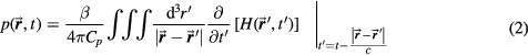
where the coordinate system is shown in figure 1. In equation (2), two shifted time variables are introduced: t is the time variable at the detector (at  ) and t' is the time variable at irradiated point
  . Given that the speed of protons and cascading electrons is much greater than the speed of sound, cradiation » c, and the timescale of conversion from radiation to heat is on the order of
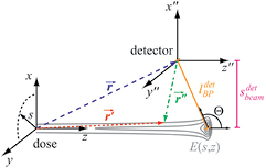
Figure 1. The proton beam energy deposition, E(s,z), is plotted in the xz plane. The pressure measured at detector position  is related to the integral over all dose volume at
  (equation (2)). The time at the detector, t, is retarded relative to the time at
  , t', by
  . The x''y''z'' coordinates are defined and centered on the detector.
  .
.  is the distance between the detector and Bragg peak.
  is the lateral distance between the detector and dose deposition axis (z). Θ is the angle between z and a vector originating at the Bragg peak.
Download figure:
Standard image High-resolution image10−12 s, the local heating induced by the proton pulse is assumed to be instantaneous. t and t' share a common 0 defined by the arrival time of the proton pulse. The acoustic waves emitted from  at t' will reach the detector at
  .
.
The energy deposition rate is separable into a time-dependent function, E(t') [J s−1], and a spatial energy deposition, E(s,z) (m−3), where, due to the cylindrical symmetry of the proton pencil beams considered here, s = (x2 + y2)1/2 is used:

E(s,z) is a relative quantity whose volume integral is normalized to 1; for a total input energy ( ), the fraction that is deposited within a voxel is given by the integration of E(s,z) over that volume. Because the simulation is computed assuming a homogeneous volume, the cumulative dose deposition, D(s,z) [Gy], is given by integrating over the full proton pulse and dividing by the density:
 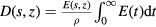 . Therefore the spatial dose deposition is proportional to the spatial energy deposition. Because the heating is assumed to be instantaneous, then E(t') = E(t) is equal to the proton pulse (in units of J s−1). Proton sources operate by modulating a stream of nanosecond proton 'micro'-pulses, whose periods (often <10 ns) are much faster than the transit time of sound across dose deposition length scales of interest (1 mm/c = 700 ns » 10 ns). Therefore, the temporal 'micro'-structure is not relevant to this discussion, and, instead, all discussion of proton pulse widths or characteristics refers to the 'macro'-structure modulating envelope.
Equation (2) can be simplified into two equations (see appendix


Pδ is introduced because it is at the heart of calculating the pressure. Equation (4) is written without simplifying and pulling tc out of the integral to highlight the physical meaning of Pδ—it is proportional to a spherical surface integral of the spatial energy deposition divided by the radius, E(s,z)/R'', where R'' = tc is the radius of a sphere centered at the detector. The 1/R'' in equation (4) is due to the radial dependence of the pressure amplitude, which drops off with the inverse of the radius (the energy/s is proportional to pressure squared, which, in accordance with the inverse-square law, scales with 1/R''2). The symbol Pδ is chosen to highlight its relationship to the pressure. Working back from equation (5), when a Dirac-delta-function (δ-function) proton pulse is substituted into equation (5), it collapses to 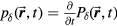 . Thus, Pδ is the indefinite integral (with respect to time) of the detected pressure generated by an impulsive, proton pulse (with infinitely small pulse-width). Based on this description we can build an intuitive understanding of Pδ. When a δ-function proton pulse irradiates a homogeneous volume, it creates a source pressure proportional to the energy deposition, E(s,z). Each irradiated source pressure volume element emits a micro bipolar pressure wave. The pressure measured at the detector (pδ) is the sum of the micro pressure waves emitted by each volume element. Because of the constant sound speed throughout the medium, from the detector's perspective, the pressure that arrives at a certain time t is related to the pressure waves emitted at a common radius (R'' = tc). Thus, Pδ, a spherical surface integral over the deposited energy (or source pressure), correlates with the expected pδ that arrives at the detector; due to the derivative relationship, peaks in Pδ translate into bipolar pressure waves in pδ. This discussion reduces to a simple observation: if the spherical surface integral (Pδ) peaks at a radius that does not pass through the maximum Bragg peak volume, then the pδ pressure wave arrival time will be offset from the expected arrival time (distance to BP divided by c), which translates into TOF range error.
The above discussion was focused on the pressure waves that result from δ-function proton pulses. Equation (5) is general to any proton pulse. For non-δ-function proton pulses, the pressure measured at the detector is equal to the first time derivative of the convolution of the proton pulse (E(t)) with Pδ.
2.2. Protoacoustic simulations
As the first step in simulating the protoacoustic pressure waves, to determine the manifestations of irradiating with different proton pulses, equation (4) was used to discretely, numerically calculate the Pδ in water (the double integral was summed over θ" and φ'' with steps of dθ'' and dφ'' ⩽ 0.01 rad) for a grid of detector positions: s = 0–100 mm in 5 mm steps and z = 4–309, 334–709 mm in 5 mm and 25 mm steps, respectively. Given the cylindrical symmetry of the dose deposition, this 2D planar grid of detectors is equivalent to a 3D array of detectors covering a cylinder of radius s = 100 mm and length z = 709 mm. An ideal, point detector was assumed. Pδ was calculated with Δt = 100 ns time steps (Δt*c = 148.1 μm) with c = 1481 m s−1, which was chosen to match the sound speed in water at 20 °C. For E(t), different Gaussian proton pulses with full-width half-max (FWHM) of  and a maximum instantaneous amplitude of 300 nA proton current (1.87 × 10¹² protons s−1, 44.9 J s−1) were then substituted into equation (5) to calculate the simulated pressure, p. Single Gaussian pulses of
  = 1.4 and 56 μs deposit 1.1 and 43.3 cGy (2.8 × 10⁶ and 1.1 × 10⁸ protons) per pulse. Calculation of each Pδ took ~100 s on a personal computer. Thus, the pressure simulations were performed by first calculating Pδ (equation (4)) and then substituting it into equation (5) with the specified proton pulse, E(t).
The 300 nA instantaneous proton current limit was chosen to assess the pulse length effect on protoacoustic amplitude because we anticipate that proton sources will be limited by maximum current, either due to safety restrictions (which are really intended to limit average proton current rather than instantaneous current (Jones et al 2015)) or instrument capacity (there is an upper limit to the proton current output). The simulations are therefore meant to reflect the situation in which the operator has control over the pulse shape but is limited to an instantaneous proton current ceiling. Another logical approach is to simulate various pulses with equivalent protons per pulse. Conversion to this framework is straightforward: for a particular proton pulse, the pressure amplitude is proportional to the number of protons per pulse (which is also proportional to  : the dose deposited at the BP by a single 300 nA pulse = 0.77 cGy/μs *
 ). This analysis is also included in the plot of the amplitude as a function of dose (see figure 4 below).
For clinical relevance, the spatial energy deposition for a 150 MeV proton pencil beam was used. The energy deposition, E(s,z), was calculated analytically based on empirical measurements using
This equation separates the dose deposition into the product of the lateral profile and the depth profile. Along the depth, the characteristic proton Bragg peak is described by IDD(z), the integrated dose deposition of a pristine Bragg peak with maximum dose deposited at 14.9 cm (Bortfeld and Schlegel 1996, Bortfeld 1997). The lateral profile is given by a cylindrically-symmetric Gaussian profile along s. The investigated proton beam's diameter increases with penetration (until the BP depth) due to scattering, which is captured by  , the depth dependent lateral Gaussian FWHM. IDD(z) and
  are both drawn from experimental measurements(Lin et al 2014), and they are shown in figure 2. The
  is beam-line specific. We use the parameters measured at the Roberts Proton Therapy Center at the University of Pennsylvania(Lin et al 2014). The denominator terms in equation (6) are included for normalization so that
  . The proton energy distribution is shown in the xz plane in figure 3(a).
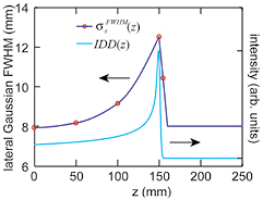
Figure 2. IDD(z) (Bortfeld and Schlegel 1996, Bortfeld 1997) and  (Lin et al 2014). IDD(z) peaks at z = 14.9 cm and has a Bragg peak FWHM along z,
  , of 7.8 mm. The experimentally measured lateral Gaussian spot profile FWHM,
  , are indicated with (o) while the interpolated values are shown with the solid line. Based on
  , the proton beam diverges: the Gaussian FWHM spot diameter expands from an initial 8 mm to ~12.5 mm at the BP.
Download figure:
Standard image High-resolution image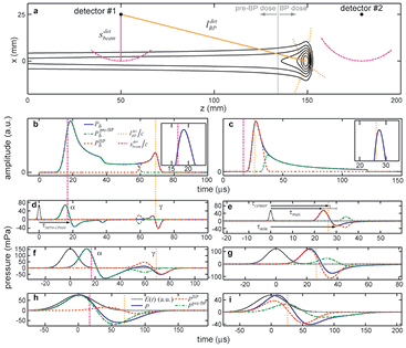
Figure 3. (a) The energy deposition in the xz plane, E(s,z), and two characteristic detector positions are plotted (#1: s = 25, z = 50 mm; #2: s = 25, z = 179 mm). To distinguish the contributions from the pre-Bragg peak and Bragg peak portions of the dose deposition (E(s,z) on left and right side of gray dashed line at z = 13.4 cm, respectively), the Pδ and p generated by these two regions are calculated and plotted separately (z = 13.4 cm or 90% of the BP range is arbitrarily chosen as the separation point). Pδ, a precursor to calculating the pressure, is calculated by taking the spherical surface integration of the energy deposition (scaled by the distance). The surface integrated shells corresponding to radii of interest R'' =  and
and  (equation (4)) are shown for each detector (dashed lines) in the xz-plane. The Pδ for detector #1 (b) and #2 (c) are plotted. The pressure simulated for Gaussian proton pulses of
  = 1.4, 14, and 56 μs are shown for detector #1 ((d), (f), (h)) and #2 ((e), (g), (i)). The
  = 1.4 μs Gaussian pulse is δ-function-like, and the pressure traces shown in (d) and (e) are approximately equal to the traces generated by an impulsive proton pulse, pδ. (b) and (d) are plotted on the same time axis to show that
  . The goal of protoacoustics is to identify
  and (to a lesser degree)
  based on the wave arrival time, τ.
  /c and
  /c are indicated by dashed lines throughout. The (b) and (c) inlays show the offset between the Pδ peak and
  /c and
  /c, respectively. This offset results in inherent distance calculation errors (eg, none of the arrival time metrics correspond to
  /c in (e)). Different arrival time metrics are shown in (d) and (e).
Download figure:
Standard image High-resolution imageTo summarize the above, using the energy distribution from figure 3(a), Pδ(t) was calculated for various detectors (at positions  ). Then, from Pδ(t), p(t) was calculated for each detector as a function of variable proton pulses (
 ). From these data traces, different measures were collected to assess the amplitude, frequency, and range verification accuracy. Table 1 lists the data and features measured for analysis. To understand the amplitude dependence, the maximum pressure, pmax, was measured from each p(t). To assess the frequency dependence, the time-domain pressure traces were Fourier Transformed, and the spectral peak frequency, ωmax, and width,
  , were measured. To understand the range verification accuracy, the arrival time of different features was measured as described below.
Table 1. The simulation data and extracted information for each study. Simulation data was calculated at various detector positions ( ) and for Gaussian excitation proton pulses of various widths (
 )
)
| Study | Simulation data | Extracted information |
|---|---|---|
| Amplitude |  |
pmax |
| Frequency | ![$|FT\left[\,p(t)\right]|$](https://content.cld.iop.org/journals/0031-9155/61/6/2213/revision1/pmbaa15a4ieqn051.gif) |
ωmax,  |
| Range verification accuracy | Pδ(t) |  |
 |
τcenter, τmax, τmin, τzero-cross |
2.3. Arrival time metrics
The TOF calculation of distance is based on the arrival time, τ, of the pressure wave of interest. In TOF calculations, the distance is calculated as the product of the speed of sound and τ. Therefore, the error in determining the distance to the Bragg peak from a TOF calculation, εTOF, is given by:

where ε is expected to depend on the detector position,  , and the proton pulse width,
  . To calculate the distance to the beam propagation axis,
  , then τα is used in place of τγ. Because simulation data is noiseless, the error (ε) is a standard error. Initial analysis of the results plots ε as a function of detector position,
  , for a particular
  . Later analysis attempts to map a more complicated exponential relationship between τγ and
  for particular
  without considering
  .
.
Because each protoacoustic pressure wave consists of a bipolar combination of a positive compression peak followed by a negative rarefaction peak, there are multiple metrics to determine τ. Considered arrival times metrics are indicated in figures 3(d) and (e). τmax and τmin are the arrival times of the compression and rarefaction peaks, respectively. τzero-cross is the time when the pressure wave crosses zero between τmax and τmin. τcenter is the average of τmax and τmin.
2.4. Noise considerations
The simulation calculates a noiseless dataset. In experiments, however, averaging is essential to remove random electrical, acoustic, and thermal noise because of the low levels of protoacoustic signals. To understand the manifestations of noise, two analyses were performed, one to investigate the signal-to-noise ratio (SNR) and another to assess how noise affects the calculation of arrival times. The effects of random noise on SNR are well established, and the noiseless simulation data was analyzed using the analytic equations below. The effect of random noise on determining arrival times is more complicated, however, and measurements of τ were repeated with noise added to the simulation data to empirically assess the manifestations.
2.4.1. SNR.
Using pmax from the simulations, the SNR was assessed for a hypothetical experimental random noise level using the analytical equation (8). If the random noise has a single measurement standard deviation of N, then the SNR resulting from averaging the protoacoustic signal resulting from n averages is given by:

where pmax is the maximum protoacoustic signal amplitude resulting from a single proton pulse measured at the considered detector. For n proton pulses, the total dose at the Bragg peak,  , is the product of n with the dose at the Bragg peak from a single proton pulse,
  . Clinically, the number of protoacoustic traces that can be averaged is limited by the total dose deposited at the Bragg peak. The ratio of SNR to
  is given by:
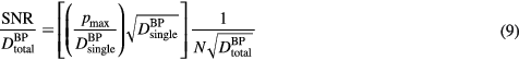
From a detection stand point, the ideal proton pulse sequence is the one that maximizes the SNR while delivering the prescribed dose  . pmax and
  depend on the Gaussian proton pulse width (
 ) while
  is a constant specific to the patient's prescribed dose (typically between 1.8 and 2.5 Gy per fraction).
2.4.2. Arrival times in the presence of noise.
In an experiment, once a sufficient SNR is achieved through averaging (see above), noise will also affect the accuracy of determining arrival times (arrival time metrics). To assess the error in measuring τ in the presence of random noise, random Gaussian noise (N) with standard deviation of 10% of pmax was added to p(t), and τ was measured. The process was repeated 100 times to gather statistics on how τ is affected by the random noise. This represents the case where SNR = 10, which was chosen a priori as an attempt to represent an intermediate SNR. The SNR depends on many experimental variables ( , maximum instantaneous current, N,
  ), and we are unaware of any experimental protoacoustic report of a typical SNR achievable within the constraints set by a limited
  . Simulations predict that random noise is <30 mPa (Ahmad et al 2015).
3. Results
Figure 3 shows characteristic Pδ (the spherical surface integral over the energy deposition scaled inversely by distance) and pressure traces simulated for two detectors, one placed in the pre-BP region and one in the post-BP region. Figure 3(a) shows the position of each characteristic detector. Figures 3(b) and (c) plots the Pδ for each detector. To understand the origin of the pressure signal, the spatial energy deposition was split into two portions: the pre-BP dose and the BP dose. Pδ is shown as the sum of the contributions from each of these separate dose regions. The Pδ shown in figure 3(b) (from the pre-BP detector) has two peaks: the earliest arriving peak is due to the pre-BP region of E(s,z) while the later arriving peak is due to the BP region of E(s,z). The Pδ shown in figure 3(c) (from the post-BP detector) has a single peak due to the BP region of E(s,z). Vertical dashed lines indicate the Pδ(t) that results from the spherical surface integral of E(s,z)/R'' at the radii R'' =  and
and  shown in figure 3(a). The Pδ peak maximum time differs from
  by 1.8 μs in figure 3(b) and differs from
  by 1.1 μs in figure 3(c), as is shown in the figure inlays.
Figures 3(d)–(i) show the protoacoustic pressure traces, p(t) (simulated by substituting Pδ into equation (5)), measured at the detectors shown in figure 3(a) after irradiation with Gaussian proton pulses with FWHM pulse-widths of  = 1.4, 14, and 56 μs. These pulse-widths are chosen to highlight characteristic regimes in which the proton pulse characteristics have negligible, moderate, and extreme effects on the protoacoustic signal. The 1.4 μs proton pulse (10–90% rise time of 1 μs) is a δ-function-like pulse. The characteristic pressure trace shown in figure 3(d) is similar to previously reported simulations (Jones et al 2014) and experiments (Albul et al 2004). Two bipolar waves are identified in figures 3(d) and (f): the α wave (bipolar wave generated by the pre-Bragg peak cylindrical energy deposition) precedes the γ wave (generated by the Bragg peak volume). For the detector placed in the post-BP region, only the γ wave is observed (figures 3(e), (g), (i)). For each bipolar wave, the initial positive feature is the compression peak while the following negative feature is due to rarefaction (expansion).
As the proton pulse  increases, the pressure peaks broaden. For a proton pulse-width of 56 μs (figure 3(h)), the broadening causes a merging overlap of the α and γ waves, which are distinguishable at shorter pulse-widths. The maximum amplitude also depends on the proton pulse-width
  , although the trend is not monotonic: of the three pulse-widths, the maximum pressure amplitude is observed for the 14 μs pulse-width (10.8 cGy/pulse at the Bragg peak)—the 1.4 μs pulse (1.1 cGy/pulse at the Bragg peak) does not deposit enough heat to generate a large pressure emission while, despite depositing the most dose (43.3 cGy/pulse at the Bragg peak), the slow rise time for the 56 μs pulse (small first derivative magnitude) results in decreased pmax relative to the 14 μs case.
For the pressure trace resulting from δ-function irradiation,  , each τ metric measured from pδ (figures 3(d) and (e)) can be traced back to a corresponding feature in Pδ: τmax and τmin correspond to the maximum and minimum derivatives of Pδ, τzero-cross corresponds to the peak(s) of Pδ, and, if the Pδ peaks are symmetric (the maximum and minimum derivatives are equally offset from the peak maximum), then τcenter = τzero-cross. Therefore, the origin of the pressure wave arrival time can be traced to Pδ. As an example, when the Pδ peak maximum is offset from
  , the τzero-cross will also be offset, which results in εTOF (equation (7)).
Figure 4(a) plots the maximum pressure amplitude (pmax) simulated for a detector placed along the beam propagation axis and 5 cm beyond the Bragg peak as a function of the rise time of a proton pulse with a maximum instantaneous current of 300 nA. Two types of proton pulses were considered: Gaussian (the focus of the paper) and rectangular. For the Gaussian proton pulses, the amplitude increases as the proton pulse rise time increases until a rise time of 2.9 μs ( = 4.0 μs), after which the amplitude decreases towards an asymptote of 0 Pa. For comparison, when a rectangular proton pulse was simulated, the maximum pressure increases monotonically as the rise time decreases. The number of protons per Gaussian pulse is also plotted along with proportional axes indicating
  .
.

Figure 4. (a) The maximum pressure measured at a detector placed 5 cm distal to the BP (s = 0, z = 199 mm) is plotted as a function of 10–90% rise time (t10–90%) of the initiating Gaussian proton pulse (solid line) or rectangular proton pulse (dashed line). The maximum instantaneous current for the proton pulses is 300 nA. The number of protons per Gaussian proton pulse is also plotted with another axis showing the dose deposited at the Bragg peak for a single Gaussian pulse,  . We calculate a dose of 3.88 cGy is deposited at the Bragg peak per 1 x 10⁷ protons. (b) The maximum pressure per
  is plotted (
 ). From the simulations of 300 nA Gaussian proton pulses in (a), the SNR per total dose at the BP is also plotted (see equation (9)). Horizontal arrows in (a) and (b) indicate the corresponding vertical axes. (c) The inlay shows the
  (same units as right vertical axis of (b) for
  = 2 μs as a function of proton current. The overlaid dotted line indicates a square root dependence on proton current.
Download figure:
Standard image High-resolution imageFigure 4(b) shows the maximum amplitude per Bragg peak dose for single Gaussian proton pulses of varying width ( ). The
  plot shows the
  -dependent pressure trend that is observed if each proton pulse has an equivalent number of protons per pulse (rather than the case where the max current is 300 nA for each pulse, shown in figure 4(a)). For
  , as the proton pulses are shortened, the maximum pressure per dose at the Bragg peak increases until it asymptotes to the value for a δ-function irradiating proton pulse. Also plotted is the SNR per total dose at the BP resulting from averaging the pressure measured following irradiation with multiple proton pulses. The
  peaks at
  = 2 μs for this detector position. As the proton current (protons / pulse) is increased, the functional form of
  does not change, and it peaks at
  = 2 μs regardless of current. An inlay, figure 4(c), displays the square root dependence of
  at
at  = 2 μs for proton currents 0–600 nA (0–8 × 10⁶ protons/pulse).
Figure 5 shows how the maximum simulated pressure decreases as a function of distance from the dose deposition. Lateral to beam propagation axis, the pre-Bragg peak deposition radiates pressure waves with ~s−0.5 amplitude dependence. Beyond the Bragg peak but close to the beam propagation axis (Θ ⩽ 20°), the amplitude from the BP dose deposition drops with ~ −0.96.
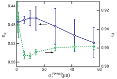
Figure 5. The results of fitting the maximum pressure measured as a function of distance. Solid line—for the pre-BP dose region (z < 13.4 cm), the maximum amplitude drops off along s with a relationship  . The errorbars show the standard deviation from averaging the ns calculated based on fitting each line of detectors at constant z. Dashed line—for the BP dose region (z > 13.4 cm), the maximum amplitude measured with Θ < 20° drops off along l with a relationship
  . The errorbars show the standard deviation from fitting nl to all of the data.
Download figure:
Standard image High-resolution imageFigure 6(a) shows the sum of pressure wave spectra simulated at each considered detector position for different irradiation proton pulses. Given the limited bandwidth of transducers, spectral information such as this is important for determining which detector to use experimentally. Figure 6(b) plots the spectra simulated at a detector distal to the BP for different proton pulses. Figure 6(c) plots the frequency of maximum magnitude, ωmax, and spectral FWHM,  , from the summed spectra in figure 6(a). As the proton pulse-width increases, the frequency of maximum magnitude decreases from 44.5 kHz. There is a negligible change in the spectra for proton pulse
  ⩽ 1.4 μs, and there is negligible magnitude above 500 kHz. The spectrum of the sum of responses from all detectors for
  = 0.1 μs (figure 6(a)) drops to −3 dB at 90 kHz,−20 dB at 240 kHz, and −38 dB at 500 kHz. For a single distal detector (figure 6(b)), the spectrum drops to −3 dB at 210 kHz,−20 dB at 390 kHz, and −37 dB at 500 kHz.
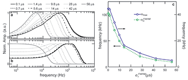
Figure 6. (a) The normalized sum of the protoacoustic frequency spectra measured at each detector position (![$\mathop{\sum}^{}|FT\left[\,p(t)\right]|$](https://content.cld.iop.org/journals/0031-9155/61/6/2213/revision1/pmbaa15a4ieqn100.gif) ). (b) The frequency spectrum of the protoacoustic γ peak measured at detector (s = 0, z = 309 mm). (c) The maximum frequency, ωmax, and spectral FWHM,
). (b) The frequency spectrum of the protoacoustic γ peak measured at detector (s = 0, z = 309 mm). (c) The maximum frequency, ωmax, and spectral FWHM,  , observed in (a). The
  is plotted on the left axes while the ωmax is plotted on the right.
Download figure:
Standard image High-resolution imageFigure 7(a) plots the systematic error for calculations of the distance between the detector and Bragg peak based on when Pδ peaks. This error was calculated as follows (see equation at top of figure 7(a)). A detector was placed at each pixel position. For each detector, the Pδ was simulated, and the time when Pδ peaks ( ) was used as the arrival time to calculate the BP to detector distance (
 ). The actual distance (
 ) was subtracted from this calculated distance to give the plotted systematic error,
  . Note that there is no
  dependence to this error because Pδ is a simulation precursor independent of proton pulse characteristics. Therefore,
  provides a best-case-scenario for experimental observations. The maximum magnitude of this error is 2.6 mm, and the angular dependence is shown in figure 7(b).
Figure 7. (a) The systematic error in determining the Bragg peak distance,  , based on the time when Pδ peaks (
 ). The color at each position indicates the error simulated at a detector at that coordinate. For example, as shown in the inlay of figure 3(c), for a detector at (s = 25, z =179 mm), even without the error introduced by a finite proton pulse width, the γ wave will arrive 1.1 μs later than the actual
  , which results in a systematic 1.6 mm error in TOF Bragg peak distance determination. The white vertical line at z ~ 315 mm is a residual of plotting caused by the change in detector spacing from Δz = 5 to 25 mm. (b) The systematic error plotted as a function of Θ, the angle between the BP and the detector. The solid line indicates a fit to the difference of two Gaussian functions.
Download figure:
Standard image High-resolution imageThe error in the TOF-based calculation of the Bragg peak distance simulated for proton pulses of various  is shown in figure 8. For these calculations, the arrival time was calculated from the simulated p(t) arrival time metrics (not directly from Pδ, as in figure 7). For the 1.4 μs proton pulse, the simulated
  matches the error from
  , and there is an angular dependence. The error ranges from −2.7 to 2.6 mm over the sampled space, with ~0 mm error distal to the Bragg peak (with Θ < 20°). For the 14 μs proton pulse, the error retains some angular dependence, but beyond the Bragg peak the error is a constant 4.6 mm. For the case of a 56 μs proton pulse, the error increases as a function of
  up to 23 mm.

Figure 8. The error in the TOF determination of distance to Bragg peak ( ) for different proton pulse widths.
  is determined from the simulated pressure traces, p(t) (as illustrated in figure 3(e)). For b + c, the errors at z < 14.9 cm are multiplied by −1. The white space in this region indicates where α and γ wave overlap prevents determining the γ wave arrival time,
  . The white vertical line at z ~ 315 mm is a residual of plotting caused by the change in detector spacing from Δz = 5 to 25 mm.
Download figure:
Standard image High-resolution imageThe goal of protoacoustics is to convert an experimentally determined arrival time to a distance to the Bragg peak. As is shown in figure 8, for some cases, systematic  errors undermine simple TOF determinations of the distance. To reduce the systematic errors, the
  -dependent
  values were fit to an exponential function:

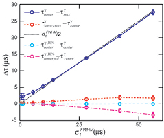
where c is the speed of sound and f, g, and h are fit parameters. Figure 9 shows the residual error in mapping  to the arrival time, τcenter, using equation (10) and parameters described in table 2. As the proton pulse
  increases, the necessary mapping correction also increases. Over the considered detector positions, the mapping results in <5 mm (
 = 56 μs, figure 9) error, which is a decrease compared to the simple TOF systematic error, which was > 20 mm (
 = 56 μs, figure 8(c)). If the detector is placed distal to the Bragg peak and within Θ < 30° from the beam propagation axis, the standard deviation (calculated from systematic error residuals shown in figure 9) in determining the Bragg peak distance based on equation (10) is <0.5 mm (tabulated in table 2).
Table 2. The arrival time was mapped to the distance between detector and Bragg peak using equation (10). Only the data simulated for detectors in the post Bragg peak region (z > 14.9 cm) was used in the least squares fitting routine to determine f, g, and h. When a value is not given, the parameter was not used in the fitting routine. The final column corresponds to the  error calculated for a detector positioned at z = ∞, s = 0. For example, for (s,z,
  ) = (0,∞,56 μs),
  =
=  − 24.58 mm.
 (μs) (μs) |
f (mm) | g (μs) | h (mm) | Std. dev. for Θ < 30° (mm) |  (z = ∞, s = 0) (mm) (z = ∞, s = 0) (mm) |
|---|---|---|---|---|---|
| 0.7 | — | — | — | 0.31 | 0.30 |
| 1.4 | — | — | — | 0.30 | 0.15 |
| 5.6 | — | — | 1.80 | 0.24 | 1.19 |
| 9.8 | — | — | 3.17 | 0.15 | 2.81 |
| 14 | — | — | 4.60 | 0.10 | 4.59 |
| 28 | 5.27 | 49.7 | 10.25 | 0.27 | 10.37 |
| 42 | 9.80 | 59.0 | 15.85 | 0.41 | 16.29 |
| 56 | 15.92 | 69.1 | 22.67 | 0.50 | 24.58 |

Figure 9. The residual from fitting the detector to Bragg peak distance,  , with equation (10) and values given in table 2. Only the data simulated for detectors in the post Bragg peak region (z > 14.9 cm) was used for determining the variables in table 2. The black data points indicate the detectors with Θ < 30°.
Download figure:
Standard image High-resolution imageFigure 10 compares the different arrival time metrics relative to τcenter. For Gaussian irradiation proton pulses, τzero-cross matches τcenter. τmax is offset from τcenter. τmin is not shown because it is equally and oppositely displaced from τcenter as τmax. The standard deviation error in calculating τcenter after 10% random Gaussian noise is added to the pressure trace is negligible. Calculating τcenter from traces with 10% Gaussian noise with a Wiener deconvolution produces larger standard deviation error (up to 4.5 μs).
Figure 10. The difference between arrival time metrics are plotted as a function of proton pulse  . Simulated data from detectors placed in the post-BP region were used (z > 14.9 cm). The error bars correspond to the standard deviation of the indicated quantities measured over all considered detector positions. In the presence of 10% Gaussian noise, the standard deviation for determining the
  at each detector is less than 0.5 μs. The standard deviation error bars for
  −
−  are negligible.
  is the arrival time calculated with the Wiener deconvolution after adding 10% Gaussian noise to p(t).
Download figure:
Standard image High-resolution image
4. Discussion
Based on the observed amplitude, frequency, and TOF observation, it is essential to describe proton pulses as δ-function-like ( at
at  ⩽ 4 μs for this dose deposition) and longer (
 at
at  > 4 μs). Framed differently, a δ-function-like proton pulse is one that satisfies the thermoacoustic stress confinement condition: the energy deposition occurs faster than the generated pressure waves can traverse the heated volume, so the emitted protoacoustic waves depend solely on the spatial form of the energy deposition, not on the temporal characteristics of the excitation proton pulse.
4.1. Amplitude
The pmax simulated here (t10–90% = 18 μs, pmax = 70 mPa,) is on the same order of magnitude as a recent experimental report with similar beam characteristics (15–20 mPa) (Jones et al 2015). The difference in simulation and experiment may be due in part to the finite bandwidth of the detector (Ahmad et al 2015), although further experiments are necessary for further comparison.
The proton pulse with a rise time of 2.9 μs (4.0 μs  ) generates the maximum amplitude per pulse for the beam characteristics and distal detector position considered here (figure 4(a)). At shorter Gaussian
  , the compression and rarefaction features destructively interfere, which causes the drop in maximum pressure at
  < 4.0 μs. For the ~600 μs FWHM rectangular proton pulses, there is no destructive interference because of the time separation between the compression and rarefaction waves (generated by the rise and fall of the proton pulse), and the drop in maximum pressure with decreasing rise time is not observed. Agreement between the maximum amplitude for the rectangular and Gaussian pulses at long rise times indicates that the amplitude is directly related to the rise time; despite delivering different numbers of protons, rectangular and Gaussian pulses with the same rise times generate protoacoustic emissions with the same amplitudes. For example, for a proton pulse with t10–90% = 6.5 μs, a ~600 μs rectangular pulse (1.1 × 10⁹ protons, 4.29 Gy at BP) and a Gaussian proton pulse (1.8 × 10⁷ protons, 7.0 cGy at BP) generate a protoacoustic pulse with the same pmax (112 and 117 mPa, respectively). Moreover, ~600 and ~800 μs rectangular proton pulses with the same rise time generate the same pmax. Mathematically, based on the convolution shown in equation (5), the maximum protoacoustic amplitude per pulse is achieved when the Gaussian proton pulse best overlaps the compression peak of pδ. Intuitively, a δ-function-like proton pulse initiates the emission of the pδ pressure waves from the irradiated deposition volume. If the proton pulse is longer than the pδ pressure wave peak-widths, then stress confinement is not satisfied, and the heating (induced by the proton pulse) extends the pressure emission time period. If the proton pulse is shorter than the peak-widths of the pδ pressure wave, then less energy is deposited and the amplitude is lower than ideal. If the proton pulse matches the peaks of the pδ pressure wave, then the protoacoustic emission amplitude is maximized without broadening the pressure signal. Plotting pmax as a function of
  for different detector positions (not shown) reveals the same trend as in figure 4(a), but pmax peaks at different
  (for figure 3(a) detectors #1 and #2, pmax peaks at
  = 8 and 7 μs, respectively). This is because the pδ pressure waves have different widths depending on the detector's orientation relative to the proton beam, which will match different width proton pulses.
Although the amplitude per pulse (pmax) has a non-monotonic dependence on rise time, the ratio of protoacoustic amplitude per deposited dose ( ) monotonically increases as the Gaussian proton pulse shortens (equivalently, as the rise time becomes faster) (figure 4(b)). Because both pmax and
  are proportional to the maximum instantaneous proton current (300 nA here), their ratio,
  , is independent of the proton current magnitude (and the number of protons per pulse). Fast rise time proton pulses, however, may not lead to the highest signal-to-noise ratios per total deposited dose. In previous studies, averaging of the protoacoustic signal has been necessary to remove random noise (Sulak et al 1979, Hayakawa et al 1988, 1989, Tada et al 1991, Hayakawa et al 1995, Albul et al 2001, Albul et al 2005, 2004, Capone and De Bonis 2006, Graf et al 2006, Terunuma et al 2007, De Bonis 2009, Bychkov et al 2010, Assmann et al 2015). Based on the analytical equation (8), the SNR depends on the square root of the number of averages while the signal per Gaussian proton pulse peaks at
  = 4.0 μs. Once both of these effects are considered (equation (9)), the SNR per total dose peaks for a Gaussian proton pulse with
  of 2 μs (figure 4(b)). Clinically, if the signal from many proton pulses is averaged, this study indicates that a 2 μs Gaussian proton pulse will provide the highest SNR per total dose relative to other Gaussian pulses (for this detector position). Because the
  term depends on the proton current magnitude, the
  will also exhibit a square-root proton current dependence (higher proton currents translate into higher
  ), as is shown in figure 4(c). For other beam characteristics, detector positions, and non-Gaussian proton pulse shapes the
  may peak at different values. For detectors #1 and #2 from figure 3(a),
  peaks at
  = 4 μs.
Based on the pressure trace simulated at (s,z) = (0,709 mm), approximately ~10−11 of the total deposited proton beam energy is converted into protoacoustic pressure waves. This protoacoustic energy is calculated by assuming the pressure is a spherical wave originating at the BP through  . The ratio of protoacoustic pressure energy to deposited proton energy is largest at
  ~ 2 μs. This is consistent with the above discussion: when the proton pulse matches the pδ(t) acoustic peaks, energy will be most efficiently transferred
For a mono-energetic proton pencil beam, the dose deposition can be approximated by a pre-Bragg peak cylinder and a Bragg peak disc(Jones et al 2014). The cylinder segment emits pressure waves that exhibit a s−0.5 amplitude fall off in the radial direction, which is expected for a cylindrical antenna(Sulak et al 1979)(figure 5(c)). Along the beam axis, distal to the Bragg peak, the disc segment emits pressure waves that exhibit an  −0.96 amplitude fall off, which is close to the r−1 behavior expected for a point source(figure 5(c)). Because the pressure waves are a linear combination of the contributions from each separate segment, the amplitude falloff for the full dose deposition will exhibit a more complicated behavior.
4.2. Frequency
Characterizing the frequency spectrum through simulation allows for proper selection of detectors. In particular, cutting out high frequency components either through inappropriate filtering or the use of bandwidth-limited detectors will broaden time-domain protoacoustic peaks, which may skew the measurement of arrival times (and BP positions). Exclusion of low frequency components is expected to be less drastic. Understanding the spectrum also allows for future assessment of protoacoustic wave propagation through tissue, which is frequency-dependent.
As the proton pulse rise time lengthens, the average protoacoustic spectrum decreases in frequency. The protoacoustic frequency spectra for proton pulses with  ⩽ 1.4 μs (⩽1.0 μs rise times) are indistinguishable, which indicates that the these shorter pulses are δ-function-like. For proton pulses with
  ⩾ 5.6 μs (⩾4.0 μs rise times), the longer rise times are blurring out sharper features in Pδ. Even for the δ-function-like proton pulses, there is negligible amplitude above 500 kHz, and the frequency spectrum peaks at 45.5 kHz.
The frequency, ω, of the protoacoustic spectrum is expected to be defined by the lesser of either the proton pulse FWHM (ω ~ 1/ ) or the transit time of sound across the dose deposition: ω ≈ 1/ (
 ) for detectors placed in the pre-Bragg peak region or ω ≈ 1/ (
 ). From figure 6(b), the frequency spectrum from the protoacoustic signal simulated at a detector placed at (s = 0, z = 309 mm) peaks at 100–200 kHz for a δ-function-like proton pulse, which is consistent with the prediction (ω(
 = 7.8 mm) ≈ 190 kHz). As the proton pulse
  increases at and above 5.6 μs, the ωmax from the single detector decreases, which is also consistent with prediction (ωmax(
 = 5.6 μs) ≈ 179 kHz); once the proton pulse
  increases beyond 1.4 μs, the maximum of the frequency spectrum becomes limited by the proton pulse time characteristics rather than the transit time of sound across the dose deposition structures. In photoacoustic measurements, short photon pulses allow for high spatial resolution of heterogeneous structures within the illuminated volume. In protoacoustic measurements, the current goal is to determine the characteristics of the dose deposition, which has millimeter-length-scale features. δ-function-like proton pulses will not limit the frequency spectrum, but using short proton pulses with
  < 1.4 μs (rise time <1.0 μs) will provide no advantage in dose deposition spatial resolution. If, on the other hand, protoacoustics was applied similarly to photoacoustics to image heterogeneous structures in the illuminated volume, then faster rising proton pulses would be required to achieve sub-millimeter resolution.
Given that there is negligible spectral amplitude at >500 kHz in both the summed spectra and the individual spectra (figures 6(a) and (b)), low frequency (<500 kHz) transducers are ideal for protoacoustic measurements of the simulated proton beam. If slower rising proton pulses are used, then lower frequency transducers are needed (or are sufficient). If lower energy protons are used, the spatial dimensions of the dose deposition  will be reduced, and proton pulses with faster rise times will be required along with transducers having higher matching bandwidths (Assmann et al 2015).
4.3. Accuracy of TOF calculation of the proton range
4.3.1. δ-function-like proton pulses.
The characteristic Pδ traces are plotted in figures 3(b) and (c) to show the origin of the protoacoustic signal. The pressure waves are generated by maxima in the spherical surface integration of the dose (Pδ). The intuitive assumption of TOF-based calculation of the range is that the arrival time of the γ(α) wave is given by  (
( ). Inspection of equation (5) reveals that the pressure detected for a δ-function proton pulse is given by pδ = ∂Pδ/∂t. Therefore, the arrival time of the pδ γ and α waves is dictated by the time when Pδ peaks. If the Pδ does not peak at
  and/or
  , as is the case in both figures 3(b) and (c), then the TOF-calculated range will be offset from the actual range. The systematic error due to this non-coincidence is shown in figure 7. The non-coincidence is due to the non-symmetric nature of E(s,z), the finite lateral beam diameter (
 > 8 mm), and the finite width of the Bragg peak (IDD(z)
  = 7.8 mm). If these characteristics could be changed, narrowing the Bragg peak width (
 ) would provide the largest reduction in inherent error for determining
  ; reducing the beam diameter would primarily improve calculation of
  . Using figure 3(c) as an example, Pδ peaks beyond
  . This is explained by inspecting detector #2 in figure 3(a); in the surface integration of E(s,z)R'', at R'' =
  the integration surface passes through the Bragg peak, but extending the radius slightly (by 1.6 mm) results in a larger Pδ because the spherical surface passes through more dose volume at the edges of E(s,z). Essentially, the asymmetry of the Bragg peak dose deposition imprints itself on the emitted pressure wave, which skews the arrival time and results in a systematic error in the TOF calculation of the range.
Given the presence of systematic error,  (figure 7), even without considering the skewing effects of non-δ-function proton pulses, calculating the range from the TOF may lead to error with a magnitude of <2.6 mm depending on where the detector is placed relative to the Bragg peak. The inherent error has a strong angular dependence with negligible error along the beam propagation axis (Θ < 20°) and beyond the Bragg peak, suggesting that some a priori knowledge of the detector position relative to the dose deposition will allow for a correction of the TOF-calculated range. The systematic error is expected to be lower in different proton beams with smaller diameters or lower energies, which decrease the Bragg peak width along z,
  . The ability to narrow the proton beam diameter, however, is limited by scattering, which causes a lateral spread.
4.3.2. Non δ-function-like proton pulses.
For non-delta function-like proton pulses (rise time ⩾ 4 μs) the TOF-calculated range error is further increased beyond the  error (compare figures 7 and 8) due to the convolution with E(t). From equation (5), the arrival time of the pressure γ and α waves will correspond to the peak(s) in
 ![$\left[E(t)*{{P}_{\delta}}(t)\right]$](https://content.cld.iop.org/journals/0031-9155/61/6/2213/revision1/pmbaa15a4ieqn187.gif) . The Pδ peaks will be further shifted and smeared by surrounding Pδ intensity due to the convolution with the proton pulse, E(t). For Gaussian proton pulses with large
. The Pδ peaks will be further shifted and smeared by surrounding Pδ intensity due to the convolution with the proton pulse, E(t). For Gaussian proton pulses with large  , the convolution mixes intensity from the pre-BP and BP Pδ, which causes a merging of γ and α waves, as observed in figure 3(h).
Therefore, as the proton pulse length increases and becomes less δ-function-like, stress confinement is no longer achieved, and the error between the estimated and actual travel time increases. For detectors beyond the BP, the pressure waves arrive later than expected (later than  ) because of overlap between acoustic pressure generated by the BP and pre-BP portions of the dose deposition. As the proton pulse rise time increases, the error loses its angular dependence (
 > 9.8 μs) and exhibits a constant error offset in the simulated z > 300 mm detector region (
 5.6 through 14 μs). The
  changes monotonically, and at larger pulse-widths, an exponential function maps the arrival time to the BP distance (table 2, figure 9), which indicates that the error depends on the distance and asymptotes to a value at infinite separation. At infinite distance between detector and dose, the spherical integration approaches planar integration and the difference between 1/R'' across the dose volume is negligible. Thus, for a detector placed at infinite distance along the beam axis, the integral in equation (4) becomes proportional to IDD(z), and the systematic asymptotic TOF range calculation error limit for a given proton pulse can be calculated through [IDD(z)* E(t)]. In table 2, this
  has been calculated to range from 0.3 to 24.58 mm for various proton pulses. Because of the sampled detector positions, the data in figure 9 (used for table 2) is dominated by low Θ values at large z (see black data points in figure 9), and the fitting functions given in table 2 asymptote to values close to the
  values calculated as described above for a detector at infinite distance on the beam axis.
Based on this analysis, the TOF range-verification error and its dependence on proton pulse rise time can be attributed to 1) inherent non-coincidence between Pδ peaks and  and 2) skewing due to the convolution with the proton pulse. For proton pulses with short rise times, where convolution skewing is not an issue, 3D filtered backprojection algorithms can be used to reconstruct the 3D dose distribution (Alsanea et al 2015). This reconstruction requires protoacoustic data acquired at many points surrounding the deposition, whereas here we assess the viability of arrival time calculations based on a single or a few detectors.
4.3.3. Simulation-based mapping.
To correct for the skewing due to convolution with the proton pulse, a mapping method demonstrates a possible technique for more accurately determining the distance to the Bragg peak based on the protoacoustic signal arrival time (figure 9). For example, for the  56 μs proton pulse, the mapping has 20–25 mm less systematic error than simple TOF-calculation (equation (7)) in the z > 300 mm distal region. With the mapping, the (systematic error) standard deviation of determining
  with detectors placed beyond the Bragg peak within a cone of Θ < 30°, is <0.5 mm, which represents a large increase in accuracy compared to direct TOF calculations. Clinically, mapping would require running simulations specific to the beam diameter, energy, and proton pulse characteristics to generate plots that correlate
  with the arrival time. Also, all simulations presented here were performed in a homogeneous water medium at 20° C. As in ultrasound, clinical mapping should be performed with c = 1540 m s−1, the average speed of sound in tissue. The error introduced by determining distance using an average speed of sound is under investigation. Using CT to provide more accurate sound speeds may increase accuracy at the expense of added complexity (Fontanarosa et al 2013).
4.4. Arrival time metrics
4.4.1. Comparison of different metrics.
Given their bipolar nature, the arrival time of the α and/or γ waves can be determined based on different measurements. For δ-function-like Gaussian proton pulses, τzero-cross corresponds directly to the Pδ peak (the spherical surface dose integration with the most amplitude after scaling by 1/R''), but for non-Gaussian pulses (for example, rectangular pulses), there may not be a clear point when the pressure traces cross zero between temporally separated positive compression and negative rarefaction peaks, and τzero-cross will be ill-defined (Jones et al 2014). τmax and τmin correspond to the maximum and minimum slope of Pδ (for δ-function-like proton pulses). If we assume that the peaks in Pδ are symmetric, then τcenter = (τmax + τmin)/2 corresponds approximately to peaks in Pδ. For Gaussian proton pulses, figure 10 shows that τcenter ≈ τzero-cross for short proton pulses (0.6 μs variation error when  = 9.8 μs). Because it is more robust to different proton pulse shapes, τcenter was used here as the arrival time for TOF calculations. It is also attractive to define a relationship between τmax and τcenter because the compression peak will be the first wave to reach the detector and the easiest feature to identify. From inspection of figure 10, for Gaussian proton pulses with
  ⩾ 9.8 μs, there is an offset between τcenter and τmax (and τmin) that roughly corresponds to the proton pulse
  /2. For longer pulses where
  is much greater than sound's transit time across the dose deposition, the (τmax − τcenter) offset is expected to approach
  , the difference between a Gaussian function's maximum and the maximum of its first derivative. For shorter proton pulses below
  = 9.8 μs, however, the (τmax − τcenter) offset asymptotes towards a value dependent on Pδ and independent of the proton pulse
  . Specifically, for δ-function Gaussian proton pulses,
  corresponds to the time when
  reaches its maximum, which is offset from the time when Pδ reaches its maximum, the feature that most closely correlates with
  . Therefore, using τmax as the arrival time for TOF calculations will result in a systematic error (~3.3 mm in this case for a
  = 0.1 μs), correction of which requires simulation. Therefore, τcenter is a more accurate and robust arrival time metric.
The arrival time metrics here are measured from the full pressure trace, p(t). Looking forward towards potential experiments, scaling up automatic data analysis techniques to process large quantities of data from multiple transducers or from unaveraged single-shot traces may require real-time analysis which extracts the desired arrival time from each trace before discarding the trace from memory. Given that the positive compression peak generally has the most amplitude, these techniques will most likely measure  (with concomitant systematic errors and offsets described above). Other arrival time features will most likely display a near constant offset from
  , and must be assessed through simulation. At present, the potential on-the-fly analysis techniques, such as nuclear physics constant fraction discrimination, are not applicable because the SNR appears to be too poor to allow analysis of single-shot traces: averaging is necessary, which requires holding many traces in memory. However, future time measurement techniques may be borrowed from other fields such as ultrasound or nuclear physics.
4.4.2. Noise.
To assess the applicability of TOF range calculations, another consideration is the effect of introducing noise into the measurement. An error of 1 μs in determining the arrival time translates into a 1.5 mm error in distance calculation. To assess the effect of noise in determining the arrival time metrics, random Gaussian noise with a maximum magnitude of 10% of the simulated pressure trace maximum was added to the simulated pressure traces. Given that the SNR is fixed for this noise study (SNR = 10), the  results are independent of protons/pulse. As an example, from the presented simulations, a SNR ⩾ 10 will be achieved at a detector 5 cm beyond the BP when the protoacoustic signal resulting from a (
 = 2 μs, max current = 300 nA) proton pulse is averaged to a
  = 2.0 Gy (n = 129 averages) if N ⩽ 147 mPa (much higher than the predicted noise of ~30 mPa (Ahmad et al 2015)). For a
  = 20 μs, N must be less than 28 mPa to achieve the same SNR under the same conditions. The τmax and τmin were determined by fitting the compression and rarefaction peaks to 5th order polynomials. 100 independent data sets were created by adding newly generated noise to the simulated pressure traces, and the fitting was performed on each data set. Figure 10 shows that the error in
  −
−  is negligible. For each detector position, the highest observed error in determining
  from the 10% Gaussian noise data was 0.5 μs. Thus, a SNR = 10 is more than sufficient to provide a precise (low standard deviation) measurement of τ. This insensitivity to noise is explained as follows. For short
  proton pulses the protoacoustic peaks are narrow, which reduces the range for potential error in determining maxima and minima. For large
  proton pulses, the polynomial fit effectively smoothes out the noise over the 0.1 μs sampled time steps. From the analysis, 10% random Gaussian noise only added <0.5 μs of random error in determining τcenter even for the case of the 56 μs FWHM proton pulse.
4.4.3. Deconvolutions.
In theory, Pδ can be calculated (and the convolution skewing can be removed) by taking the deconvolution of the protoacoustic pressure traces with the proton pulse. From the deconvolution, the TOF arrival time corresponds to the peaks in Pδ. After adding 10% random Gaussian noise to the simulated pressure traces (as described above), performing a Wiener deconvolution to determine the arrival time leads to modest improvements in error compared to direct TOF calculations based on the raw, non-deconvoluted data (figure 10—because the τcenter is systematically high, the negative values observed for  −
−  indicate increased absolute accuracy). The deconvolution method, however, is less robust than the analysis of the raw data: the deconvolution automatic fitting algorithm failed for proton pulse
  ⩽ 1.4 μs and the standard deviation in determining the arrival time for a single detector position from 100 sets of noisy data was ~4.5 μs for the 56 μs FWHM proton pulse (compared to 0.5 μs without deconvolution). Due to the instability of noisy deconvolutions, fitting the protoacoustic wave peaks with smoothing polynomials (see above) appears to be a more robust method for determining the TOF arrival time in the presence of noise.
4.5. Clinical implications
Although the analyzed simulations were restricted to Gaussian proton pulses and a 150 MeV beam with a beam-line specific diameter, the results can be generalized more broadly. Although the proton pulse was primarily identified by its FWHM,  , the rise time (τ90−10% = 0.716
 ) is the important quantity that affects the protoacoustic signal properties because the acoustic waves are related to the time derivative of the proton pulse, and the rise time is a measure of the first derivative. The proton pulses should be sorted into two categories: δ-function-like and longer. The δ-function-like proton pulses have rise times less than the transit time of sound across the dose deposition features. This restriction is known in thermoacoustics as stress confinement (Xu and Wang 2006). Within the δ-function-like range, the protoacoustic frequency spectrum and TOF-calculated range accuracy are independent of proton pulse rise time. In this case, the accuracy of calculating distance to the BP from the TOF is determined by the inherent systematic error. For the considered 150 MeV beam, the cross-over from δ-function-like to longer proton pulses occurs between
  of 1.4 and 5.6 μs (τ90-10% of 1.0 and 4.0 μs) and the systematic error limits the accuracy to ±2.6 mm (figure 7). Because of the strong angular dependence of the error, however, knowledge of the detector relative to the beam axis will provide corrections that improve that error (along the beam axis and distal to the BP, the inherent systematic error is ~0 mm).
For non δ-function-like proton pulses, increasing the rise time results in a lower frequency protoacoustic spectrum and larger errors in TOF calculations of the BP distance. Interestingly, tabulating the data from simulations allows for more accurate range calculations by fitting an exponential function that maps the BP distance to the arrival time of the protoacoustic wave. For example, for the proton pulse with  of 56 μs, mapping allows for more accurate determination of the BP distance (<6 mm systematic error) compared to simple TOF-calculation (up to >20 mm). Although mapping requires the complication of interpreting clinical results with matching simulations, other proton range verification methods such as PET and prompt gamma also rely on supporting simulations (from Monte Carlo) to interpret data (Moteabbed et al 2011, Sterpin et al 2015).
Examining the range verification accuracy in light of the low frequencies reveals an interesting observation highlighting the difference between ultrasound and protoacoustics. In ultrasound, due to the reflections inherent to measurement, the best axial resolution is defined by ~c/2ν, where ν is the frequency. In protoacoustic range verification, although lower frequency will generally translate into decreased accuracy, the same relationship between signal frequency and range verification accuracy does not apply: the arrival time of a 50 kHz protoacoustic wave can be determined to within a standard deviation of 0.5 μs (0.7 mm) for SNR = 10. Stated differently, even though the peaks in the protoacoustic signal are broad and the frequencies are low, the arrival time can be measured accurately.
Aside from TOF accuracy, the other important factor for clinical application of protoacoustic range verification is the SNR per total deposited dose.  peaks at Gaussian proton pulse widths close to, but shorter than, the turnover point between δ-function-like and longer proton pulses. Although the shape of
  plotted in figure 4(b) will not change with proton current (protons/pulse), the
  term of equation (9) imparts a square root proton current dependence on the magnitude of
  . Therefore, a maximum protons/pulse should be used to maximize
  .
.
Therefore, to retain the TOF accuracy and maximize the  , the ideal Gaussian proton pulse for generating protoacoustic emissions has a width slightly less than the width of pressure peaks in pδ. For the dose deposition considered here, for a detector placed on the beam axis and distal to the Bragg peak, the ideal
  = 2 μs.
For clinical sources that have longer-than-ideal proton pulses ( > 2 μs), there will be a reduced
  and larger range calculation errors, but simulation based mapping has the potential to reduce the error down to 2 mm in the region beyond the BP. All current clinical proton sources operate with proton pulse rise times that are classified as larger than δ-function like. Synchrocyclotron sources (
 = 7 μs(Kleeven et al 2013)) are the most promising for protoacoustic measurements given they can generate proton pulses closest to the ideal pulses identified here. It is expected that their TOF accuracy will display a ~1–2 mm systematic offset, as in the
  = 9.8 μs case, and the
  is ~0.5 of the ideal case. Specially modulated (
 = 18 μs (Jones et al 2015)) and standard cyclotrons (
 ~ 50 μs (Measurements 2007)) will display TOF errors that require mapping (see table 2), their
  will drop to 0.2 and 0.07 of the ideal proton pulse, respectively, and the high dose per pulse (19 and 54 cGy, respectively) limits the number of averages before the prescribed treatment dose is delivered. The low amplitude, high dose per proton pulse (2.2 Gy for maximum proton current of 300 nA), and low expected TOF accuracy for standard synchrotron pulses (
 ~ 200 μs (Measurements 2007)) most likely makes them untenable for clinical protoacoustic measurements. Potentially, these identified proton pulse rise times may be reduced through modifications such as the addition of deflectors or choppers (Yokota et al 1997) (isochronous cyclotrons) or pulse-picking mechanisms (Chuvilo et al 1984) (synchrotrons).
Analysis of the frequency spectra reveals that there are negligible frequency components above 500 kHz. Thus, a <500 kHz low frequency hydrophone is ideal for experimental measurements of clinical proton beams. Any proton pulse temporal structure less than the δ-function-like timescale is blurred out by the spatial dimensions of the dose deposition. Hence, the ns 'micro' structure of clinical proton beams is not apparent in the protoacoustic signal (see section 2.1).
Although clinical application of protoacoustic range-verificaiton will have to consider the manifestations of tissue heterogeneity, the presented simulations lay the ground work for understanding the effects of using different proton pulses. Tissue heterogeneity introduces attenuation, reflections, and variable sound speeds. Attenuation will reduce the amplitude, although the low (<100 kHz) frequency ensures better transmission than (>1 MHz) ultrasound waves, and tissue's higher (37° C) temperature and higher Grüneisen parameter are expected to increase initial protoacoustic amplitudes. The reflections will create complicated echoed pressure waves, but, because it is measured from the earliest arriving peak, τmax is expected to be unaffected. As in ultrasound, an average sound speed can be used to minimize the effects of variable sound speeds, although this will be a source of additional error.
The presented work considers the protoacoustic pressure wave generated by a single PBS beam with a pristine Bragg peak. During treatment, the irradiated volume is raster-scanned in layers by pristine BP beams with varying energies (depths) and intensities. In theory, given high enough SNR, the protoacoustic signal generated by each individual pristine BP can be measured by synchronizing acoustic detection with delivery. Without synchronization, the detected protoacoustic signal is the sum of the signals generated by each individual beam. Extracting information from the resulting sum is complicated (arguably impossible if the exciting proton pulse shape is variable), and would most likely require 3D arrays to map dose(Alsanea et al 2015). Given the large beam sizes and long beam-on times (10s of ms), protoacoustic detection is less promising for monitoring double-scattered proton therapy beams compared to PBS.
5. Conclusion
Simulations reveal the origin of the protoacoustic pressure waves. The protoacoustic pressure wave initiated by a δ-function proton pulse, pδ, is proportional to the first time derivative of a spherical surface integration of the dose scaled by the inverse of the radius. For arbitrary proton pulse shapes, the protoacoustic pressure wave is proportional to a convolution of the proton pulse with the pδ.
The simulations show that Gaussian proton pulses should be categorized into two categories: δ-function-like (with  < ~4 μs) and longer. For δ-function-like proton pulses, the frequency spectrum peaks at 44.5 kHz and the range-verification accuracy is limited by the Bragg peak asymmetry, which results in systematic errors with magnitudes up to 2.6 mm. Placing detectors distal to the proton beam and close to the beam axis minimizes this systematic error to ~0 mm. Negligible amplitude is observed at >500 kHz. For longer proton pulses, the frequency spectrum shifts to lower frequencies, the amplitude decreases, and the error in TOF range calculation also increases. Through simulations, the pressure wave arrival times can be mapped to Bragg peak distance to reduce the range calculation error compared to simple TOF calculations. By averaging the protoacoustic signal generated by 20 μs Gaussian FWHM, 300 nA proton pulses depositing a total dose of 2.0 Gy at the Bragg peak, a SNR = 10 is achieved assuming a previously predicted random noise level of ~30 mPa (Ahmad et al 2015). Therefore, based on simulations, the technique is predicted to be measurable under clinical conditions and dose limitations.
Based on maximizing range calculation accuracy and the signal-to-noise ratio per total deposited dose, the ideal Gaussian proton pulse has a  = 2 μs. The ideal arrival time metric is τcenter, the average of the compression and rarefaction peak arrival times. Determination of τcenter is negligibly affected by 10% random Gaussian noise.
Acknowledgments
This work was partially funded by the University of Pennsylvania Department of Radiation Oncology Pilot Grant Program.
Appendix A
Nomenclature
| α wave | The protoacoustic pressure wave generated by the pre Bragg peak portion of the proton dose deposition |
| β | Thermal expansion coefficient (K−1). Here β = 0.257 × 10⁻³ K−1 |
| BP | Bragg peak |
| γ wave | The protoacoustic pressure wave generated by the Bragg peak portion of the proton dose deposition |
| c | Speed of sound (m s−1). Here, c = 1481 m s−1 |
| Cp | Heat capacity (J kg−1 K−1). Here Cp = 4181 J kg−1 K−1 |
| D(s,z) | Spatial proton dose deposition (Gy) |
 | The dose deposited at the Bragg peak voxel by a single proton pulse (Gy) |
 | The accumulated dose deposited at the Bragg peak voxel by n proton pulses (Gy) |
 | The error in calculating distance based on τc (mm) |
| E(s,z) | Spatial proton energy deposition (m−3). E(s,z) is normalized so that its volume integration is 1 |
| E(t) | Proton pulse (J s−1). Here the maximum instantaneous proton pulse intensity is 44.9 J s−1 |
| FWHM | Full-width-half-max |
| Θ | The angle between z and a vector originating at the Bragg peak |
H( ,t) ,t) | The rate of input energy absorption that is converted to heat (J s−1 m−3) |
| IDD(z) | Proton integral depth dose. Due to normalization, its units are (m−1) |
 | Distance between the detector and Bragg peak voxel (m) |
| n | For averaging, the number of pressure traces collected and averaged following n proton pulses |
| N | The single measurement standard deviation of the random noise (Pa) |
 | Pressure trace as a function of time measured at a detector at position  (Pa) (Pa) |
 | p generated by the Bragg-peak portion of the dose deposition, D(s,z ⩾ 13.4 cm) (Pa) |
 | p generated by the pre Bragg-peak portion of the dose deposition, D(s,z < 13.4 cm) (Pa) |
 | Pressure trace generated by a δ-function proton pulse (Pa) |
| pmax | The maximum pressure measured at a detector (Pa) |
Pδ( ,t) ,t) | Indefinite integral of the pressure emission initiated by a δ-function proton pulse (Pa s J−1). Based on equation (4), Pδ is proportional to the surface integral of a sphere centered at the detector integrating the dose deposition divided by the distance |
 | Pδ for the Bragg-peak portion of the dose deposition: D(s,z ⩾ 13.4 cm) (Pa s J−1) |
 | Pδ for the pre Bragg-peak portion of the dose deposition: D(s,z < 13.4 cm) (Pa s J−1) |
| ρ | The density of the medium (kg m−3). Here ρ = 1000 kg m−3 |
 | Full-width-half-max of the Bragg peak in E(z) (m) |
 | Full-width-half-max of the Gaussian proton pulses (s) |
 | Full-width-half-max of the frequency spectrum (Hz) |
 | Depth-dependent full-width-half-max of the Gaussian lateral proton dose deposition profile (m) |
| SNR | Signal to noise ratio of the protoacoustic pressure trace (unitless) |
| s | Cylindrical coordinate perpendicular to the proton beam propagation axis (m) |
 | Lateral distance between the detector and the beam propagation axis (m) |
| τ | The arrival time of the protoacoustic pressure wave (s) |
| τγ | The arrival time of the protoacoustic γ wave (s) |
| τ10% | The protoacoustic arrival time determined after adding Gaussian noise with maximum amplitude of 10% of pmax to the simulated pressure trace,  (s) (s) |
| τcenter | The protoacoustic arrival time measured from the average of τmax and τmin (s) |
| τmax | The protoacoustic arrival time measured at the maximum of the positivecompression pressure peak (s) |
| τmin | The protoacoustic arrival time measured at the minimum of the negative rarefaction pressure peak (s) |
| τzero-cross | The protoacoustic arrival time measured when the pressure crosses 0 between the positive compression and negative rarefaction peaks (s) |
| t10–90% | The 10–90% rise time of the proton pulse (s) |
| TOF | Time-of-flight. Method of calculating distance based on the product of c and τ |
| ωmax | The frequency where the protoacoustic spectrum reaches its maximum value (Hz) |
| z | Coordinate along proton beam propagation axis (m) |
Appendix B
Starting with equation (2), we can re-define E(t) as a convolution of itself with a Dirac delta function:

Because the proton pulse propagates at the speed of light, E(t) = E(t'). Also, the derivative with respect to t and t' are the same. Based on the properties of convolutions, substitution of equation (B.1) and bringing the t terms out of the integral results in:
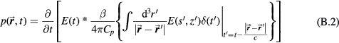
which can be rewritten as equation (5) if the second convolution term is defined as

Performing the volume integral in spherical coordinates centered at  results in:

where  . The time t is defined at the position of the detector (
 ), and tc = r''. Therefore,

The δ-function in equation (B.5) reduces the volume integral in equation (B.4) to a spherical surface integral at radius R'':

which can be re-written to give equation (4) or simplified to

which is consistent with previous reports (Paltauf et al 1998, Xu and Wang 2006).