
Abstract
Based on experiments and numerical simulations, a study is carried out pertaining to the conversion of dose-to-graphite to dose-to-water in a carbon ion beam. This conversion is needed to establish graphite calorimeters as primary standards of absorbed dose in these beams. It is governed by the water-to-graphite mass collision stopping power ratio and fluence correction factors, which depend on the particle fluence distributions in each of the two media. The paper focuses on the experimental and numerical determination of this fluence correction factor for an 80 MeV/A carbon ion beam. Measurements have been performed in the nuclear physics laboratory INFN-LNS in Catania (Sicily, Italy). The numerical simulations have been made with a Geant4 Monte Carlo code through the GATE simulation platform. The experimental data are in good agreement with the simulated results for the fluence correction factors and are found to be close to unity. The experimental values increase with depth reaching 1.010 before the Bragg peak region. They have been determined with an uncertainty of 0.25%. Different numerical results are obtained depending on the level of approximation made in calculating the fluence correction factors. When considering carbon ions only, the difference between measured and calculated values is maximal just before the Bragg peak, but its value is less than 1.005. The numerical value is close to unity at the surface and increases to 1.005 near the Bragg peak. When the fluence of all charged particles is considered, the fluence correction factors are lower than unity at the surface and increase with depth up to 1.025 before the Bragg peak. Besides carbon ions, secondary particles created due to nuclear interactions have to be included in the analysis: boron ions (10B and 11B), beryllium ions (7Be), alpha particles and protons. At the conclusion of this work, we have the conversion of dose-to-graphite to dose-to-water to apply to the response of a graphite calorimeter in an 80 MeV/A carbon ion beam. This conversion consists of the product of two contributions: the water-to-graphite electronic mass collision stopping power ratio, which is equal to 1.115, and the fluence correction factor which varies linearly with depth, as kfl, all = 0.9995 + 0.0048 zw-eq. The latter has been determined on the basis of experiments and numerical simulations.
Export citation and abstract BibTeX RIS
General scientific summary Based on IAEA TRS-398 dosimetry protocol, the absorbed dose has to be established in water. In some situations, however, the absorbed dose is determined in a material other than water and a dose conversion has to be applied to establish dose-to-water. This study is the first step of a general work based on the use of a graphite calorimeter in an 80 MeV/A carbon ion beam. In this case, the dose conversion requires water-to-graphite stopping power ratios, sw,g and a fluence correction factor, kfl. sw,g is calculated numerically, using the Geant4 Monte Carlo code, while the determination of kfl is based on both, a numerical and experimental evaluation. In general, in a low energy carbon ion beam, sw,g equals 1.115, whereas kfl increases linearly with the water equivalent depth (zw-eq), as 0.9995 + 0.0048 zw-eq.
1. Introduction
Due to their advantage in dose distribution compared to lighter ionizing particles and specific biological characteristics, the interest for ion beams in radiation oncology has been increasing for some decades (Jäkel et al 2008, Palmans 2012). At present, four clinical facilities are in operation: National Institute of Radiological Sciences/Heavy Ion Medical Accelerator (NIRS/HIMAC) and Gunma University Heavy Ion Medical Center (GHMC), both in Japan, Heidelberg Ion Beam Therapy Center (HIT) in Germany, and Hadron therapy Center for Cancer Treatment (CNAO) in Italy. Other facilities are under construction: Med-AUSTRON in Austria and one in China. More details can be found in the Particle Therapy Co-Operative Group (PTCOG) Website6. In parallel, several academic infrastructures are promoting research programmes in various nuclear science fields including dosimetry and radiobiology: this is the case of the Laboratori Nazionali del Sud of the Instituto Nazionale di Fisica Nuclear (INFN-LNS) in Catania, Sicily (Italy)7 among others. The effective clinical dose resulting from ion beam irradiation, defined as the product of the absorbed physical dose and the relative biological effectiveness (Wambersie et al 2004), is the matter of debate. The definition of mature hadron therapy practice requires efforts in both dosimetry and radiobiology, in particular, to improve the accuracy of recommended physical parameters which are included in dosimetry protocols.
Clinical dosimetry is usually based on the use of ionization chambers along with specific dosimetric protocols, such as the IAEA International Code of Practice on Dosimetry in External Beam Radiotherapy, TRS-398 (Andreo et al 2000). According to the latter, the ionization chambers have to be calibrated in terms of absorbed dose-to-water. In clinical reference dosimetry, this calibration is made with a reference device traced towards a primary standard. The main technique for establishing the absorbed dose is calorimetry (Karger et al 2010). Due to its similarities with biological tissues in the absorption properties of ionization radiation, water is the standard reference material for clinical radiation therapy (Vynckier et al 1994, ICRU 1998, Almond et al 1999, Andreo et al 2000). Consequently, water calorimeters have been developed in various standard laboratories throughout the world as primary standards for absorbed dose-to-water (Domen 1994, Palmans et al 1996, Seuntjens and Palmans 1999, Seuntjens et al 1999, Brede et al 2006). However, due to their advantages in terms of physical and chemical material properties and the precision and ease of the manufacturing process, solid calorimeters are progressively developing (Schulz et al 1990, McEwen and Duane 2000, Palmans et al 2004).
A method to decrease the uncertainties involved in dosimetry measurements in hadron therapy is the development of a primary standard. Several calorimeters have been used successfully in proton and carbon ion beams (Schulz et al 1992, Siebers et al 1995, Palmans et al 1996, 2004, Delacroix et al 1997, Sakama et al 2009, Medin 2010). At present however, although those could form the basis of primary standards, no primary standard for absorbed dose-to-water in ion beams exists. The first dedicated portable graphite calorimeter for proton and light-ion radiotherapy beams has recently been built at the National Physical Laboratory (NPL), UK (Bailey et al 2013). This graphite calorimeter will be used in future work to determine an experimental value of the mean energy expended in air per ion pair formed, wair-value, for an 80 MeV/A carbon ion beam. This quantity is needed for the calculation of the beam quality correction factors,  , used in the determination of absorbed dose-to-water in the IAEA TRS-398 protocol.
With a non-water calorimeter, a dose conversion is required to obtain the quantity of interest, absorbed dose-to-water (Palmans et al 2002, 2011, Lühr et al 2011). This dose conversion includes two contributions: first, it requires an accurate knowledge of the water to non-water material electronic mass collision stopping power ratio and second, considering differences in particle fluence distributions at equivalent depths in the non-water material and water, fluence correction factors have to be applied (Palmans et al 2013a, 2013b). For hadrons, these fluence correction factors mainly result from differences in nuclear interaction cross sections between the non-water material and water.
The research presented in this paper forms one part of a characterization of the NPL graphite calorimeter for protons and carbon ions. The objective is to present two complementary approaches to determine the fluence correction factors for graphite calorimetry in an 80 MeV/A carbon ion beam. First, the results of an experimental technique, based on the measurements of ionization curves in a water phantom and a graphite phantom, respectively, are presented. In the second part, these experimental data are compared with numerical results obtained through Monte Carlo simulations performed with the Geant4 toolkit within the GATE user interface.
2. Material and methods
In radiotherapy, absorbed dose-to-water in water Dw(zw) at a certain reference depth zw is the quantity of interest. In this study, the absorbed dose is determined in another material 'm', denoted as Dm(zm). Three steps are required to establish the relationship between these two quantities.
First, due to the difference in ranges between the two materials, the depth in the non-water material must be correctly scaled to that in water. For each particular non-water material depth zm, a water-equivalent depth zw-eq can be defined as

where r0, m and r0, w are the continuous slowing down approximation (CSDA) ranges of the incident particles in non-water and water materials, respectively. These ranges are derived as the depth on the distal edge of the Bragg peak where the dose drops to 80% of the maximum. In this paper, zw, zw-eq, zm, r0, m and r0, w will be expressed in terms of mass thickness (units: g cm−2). Secondly, a stopping power conversion needs to be applied. Thirdly, due to differences in particle fluence distributions, fluence correction factors, kfl, have to be determined.
2.1. Experimental determination: kfl, exp
The experimental results reported in this paper have been performed in an 80 MeV/A carbon ion beam produced by the superconducting cyclotron of the INFN-LNS. The used beam line, named '0 degree beam line', is composed of three devices (Cirrone et al 2011). After being scattered by a 15 μm tantalum foil, the beam exits the vacuum chamber through a 50 μm kapton window. Then, the beam is collimated through a brass tube (length = 28.5 cm, internal diameter = 36 mm, external diameter = 43 mm) including a PMMA slab (depth = 59 mm) and several brass collimators, of which the final one has a diameter of 5 mm. The last element of the beam line is a transmission chamber used to monitor the beam. The latter consists of two kapton foils with a conducting copper layer separated by 9 mm air gap.
Experimental fluence correction factors are determined as the ratio of ionization per monitor unit in water and graphite as a function of the water-equivalent depth, measured with a PPC40 parallel plate chamber, manufactured by IBA8, in a constant source-to-detector distance set-up. The assumption is made that ionization in the chamber is proportional to fluence and that fluence perturbations by the presence of the ion chamber are negligible. Since the diameter of its collecting volume (16 mm) is approximately three times larger than the diameter of the final collimator, all primary particles that are not removed from the beam due to non-elastic nuclear interactions will cross the collecting volume of the ion chamber.
Figure 1 shows the schematic experimental set-up for the measurements in the graphite phantom (top) and water phantom (bottom). The ionization curves are determined in both cases with a constant source-to-detector distance, so that the ionization chamber remains at a fixed position. The water phantom is moved using a computerized device; for graphite measurements, some graphite slabs are added or removed manually. The two situations are different in the backing. However, based on Monte Carlo simulations, for this configuration and this beam, the backscattering effects are negligible.

Figure 1. Schematic set-up for the experimental determination of ionization curves in graphite phantom (top) and water phantom (bottom). The isocentre is marked with a cross.
Download figure:
Standard image High-resolution imageAs explained previously, the comparison of ionization in graphite (g) and water (w) can be performed after establishing the ionization curves at equivalent depths in water only. Using equation (2.1), experimental fluence correction factors are given by the following expression:

where Iw and Ig are the ionization in water and graphite, respectively.
2.2. Numerical simulations: kfl, num
According to its definition, the absorbed dose-to-medium 'm' is given by the integral of the particle fluence differential in energy ϕm(E), also called the particle fluence spectrum, and the electronic mass collision stopping power of the medium Sel, m(E)/ρ, where ρ is the density. As a result of nuclear interactions and fragmentation of the primary beam, secondary charged particles are created that contribute to the absorbed dose. Consequently, absorbed dose-to-medium has to be calculated not only for primary particles but also for all charged particle types i. In this case, absorbed dose-to-medium is given by following relation:

where Emax, i is the maximum energy of particle type i.
If the particle fluence spectrum was the same for all media and all charged particle types i, based on equation (2.3), absorbed dose-to-water in the water phantom at the equivalent depths can be determined from dose-to-graphite in the graphite phantom. We can express this using the following equations:

where sw, g(ϕg) and sw, g(ϕw) represent the unrestricted water-to-graphite electronic mass collision stopping power ratio respectively for fluence in graphite and water, and is given by

Equations (2.5a) and (2.5b) are exact when (i) all charged particles are considered and (ii) the fluence distributions are obtained by tracking all charged particles down to zero kinetic energy.
In reality, the particle fluence spectrum depends on the medium. Equation (2.4) can therefore be extended with fluence correction factors that account for these fluence changes:

with
The fluence correction factors can be calculated by two different numerical approaches. The direct method consists in using equation (2.7a) or (2.7b) and to determine the particle fluence spectrum for all charged particle types in both phantoms by Monte Carlo simulations. The indirect method consists in obtaining directly the absorbed dose at equivalent depths in water and graphite by Monte Carlo simulations. Then, the fluence correction factors can be derived from


where  and
and  are given by equations (2.5a) and (2.5b), respectively.
The presented results are obtained through the GATE simulation platform (OpenGATE Collaboration 2002, Jan et al 2004, 2011). The latter, based on the Geant4 Monte Carlo code (Agostinelli et al 2003, Allison et al 2006), is an advanced open-source software toolkit developed by the international OpenGATE collaboration, dedicated to numerical simulations in medical imaging and radiotherapy. Geant4 is a general toolkit to simulate the passage of particles with matter. Its development is in a permanent evolution both in the architecture of the software and the improvement of many physical models (Batic et al 2012). There is a new release every six months approximately. This work has been performed with version 6.2 of GATE, which is combined with version 9.5.1 of Geant4.
Two types of interactions of charged particles through matter are implemented in the Geant4 simulations: electromagnetic (EM) and hadronic processes (HAD) (Apostolakis et al 2009). The first describes EM interactions between charged particles or photons with electrons or nuclei and the second describes the interactions between incident hadrons/ions and the target nuclei due to the elastic and inelastic collisions. In GATE/Geant4, users can select the most appropriate list of physical interactions according to the domain of application, types of particles and corresponding energy values; specific physics lists for hadron therapy studies have been proposed by the OpenGATE collaboration9. In order to obtain accurate simulations with an acceptable CPU time, simulations have been performed with the Standard EM energy physics list with 'Option 3' (Grevillot et al 2010, Ivanchenko et al 2011). Since in our study, no difference has been observed between recommended physics lists for applications with proton beam or carbon beam, to decrease the CPU time, results presented in this study have been obtained using the recommended physics list (EM and HAD) for applications with proton beam. The only difference with the recommended physics list for applications with carbon ion beams is the choice of the inelastic HAD model for ions: elastic interactions are managed using the G4LElastic model and inelastic interactions are modelled using the G4BinaryCascade model for protons and G4BinaryLightIonReaction for ions. Using the version 9.5.1 of Geant4, the only available class to describe the elastic scattering is G4UHadronElasticProcess.
A critical point in the Monte Carlo code is the modelling of elastic scattering for electrons and other charged particles. In Geant4, two processes are available: a single scattering algorithm (SSC), which simulates each single interaction, and a multiple scattering algorithm (MSC), which uses approximations to simulate the global effects of the collisions at the end of each step (Ivanchenko et al 2010). The latter is based on Lewis theory (Lewis 1950) and it has the advantage to exhibit a good compromise between CPU time and accuracy of simulations. Our simulations have been performed with the MSC algorithm. More details on physical models can be found in the Geant4 documentation10.
The determination of the dose deposition using Geant4 is influenced by various parameters (Grevillot et al 2010, Zahra et al 2010). Energy losses are dominated by EM interactions with atomic electrons. These energy losses are calculated using the Bethe–Bloch formula, which depends on (i) the particle, i.e. type, charge, velocity and energy, and (ii) the mean excitation potential of the target 〈I〉. The latter is a key parameter of the simulation. A number of data sets with recommended 〈I〉-values are published in dosimetric protocols. Based on the latest knowledge and experimental databases, 〈I〉-values are proposed in ICRU Report 49 (ICRU 1993). Another important parameter in Geant4 is the production cut of the simulation for the secondary particles (gammas, electrons and positrons). Below this value, no secondary particle is generated and the energy loss, which is determined using the restricted stopping powers, occurs continuously along the track. In Geant4, this cut is expressed in terms of distance (units: mm). Another Geant4 parameter to be set is the 'step limiter', which allows limiting of the maximum step size in terms of a step length. Its value has to be small enough for the cross section to be constant along the step. The choice of production thresholds and step limiters results from a compromise between accurate simulation in terms of the spatial dose distribution and available computation power.
In our simulations, water is defined as the National Institute of Standards and Technology (NIST) material G4_WATER (Arce 2009) via the internal Geant4 database, while graphite is defined as composed of carbon (100%), with a density of 1.77 g cm−3. Both for water and graphite, 〈I〉-values recommended in ICRU Report 49 have been used, respectively 75 eV for water and 78 eV for graphite. For water, other values have also been proposed. The internationally accepted values have not been settled. For example, Paul (2007) suggests a value of 80.8 ± 2 eV and ICRU Report 73 and its erratum propose 67.2 eV and 78 eV (ICRU 2005, Sigmund et al 2009), respectively. Soltani-Nabipour et al (2009) has also shown the sensitivity of depth–dose profiles to different 〈I〉-values . It was also shown in Palmans et al (2013a) that the 〈I〉-values chosen in the simulations, while they significantly impact the stopping power values, have very little influence on the fluence correction factors.
Figure 2 shows the specific model of the LNS beam line geometry used in the Geant4/GATE simulations. For the comparison with experimental data, the LNS beam line has been modelled. As described previously, the latter is composed of a scattering foil, a kapton window, several collimators and a transmission chamber. At the end, a water or graphite phantom is included. The latter is modelled by a box divided in 500 slabs with dimensions of 20 × 20 × 1.6 cm3 and 20 × 20 × 1.00897 cm3 for water and graphite, respectively. The length of the graphite phantom depends on the length of the water phantom and on the ranges of 80 MeV/A carbon ions in water and graphite. The fluence is scored at 10 slab intervals, whereas the dose is recorded in each slab.
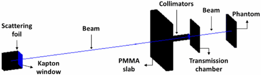
Figure 2. Components included in the geometry using in Geant4/Gate simulations: a scattering foil, a kapton window, several collimators, a transmission chamber and a phantom.
Download figure:
Standard image High-resolution image3. Results
3.1. Absorbed dose distribution
Figure 3 shows the results of simulations in graphite and water, for which the value of production cut threshold (SetCutInRegion) and the value of the limitation of the maximum size of step (SetMaxStepSizeInRegion) are different: one is performed with a production cut threshold of 107 mm and a maximum size of step of 107 mm (case 1, which gives a much reduced computation time), and the other with a 0.1 mm production cut threshold and a 0.1 mm maximum size of step (case 2, which improves the accuracy of the dose distribution). These values have been arbitrarily selected to investigate their effects on the computation time and the spatial accuracy. In both cases, the values of the step limitation are those recommended by the OpenGATE collaboration in physics lists for applications with proton and carbon ion beams11. Reduction of the maximum step value leads to an increase in computation time by a factor of 8. Both results are normalized to unity at the entrance. The difference between both cases in water and graphite is negligible. Therefore, the results presented below have been obtained with values of case 1 (SetCutInRegion = 107 mm; SetMaxStepSizeInRegion = 107 mm). Values for the parameters used in 'SetStepFunction' to control the step size of all particles have been obtained from those used in the recommended physics list for applications with proton or carbon ion beam.
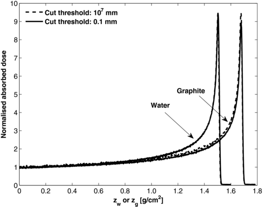
Figure 3. Numerical simulations of the absorbed dose distributions. Curves illustrate the influence of Geant4 parameters (production cut threshold and the limitation of maximum size of step) on absorbed dose computation in water and graphite. Results are normalized to unity at the entrance. Continuous lines illustrate results for the lower values of both parameters (case 1) and discontinuous lines for the higher values of these parameters (case 2).
Download figure:
Standard image High-resolution imageFigure 4 compares two carbon ion depth–dose distributions in graphite and water, respectively: one measured experimentally at INFN-LNS with the PPC40 ionization chamber and the other computed using GATE/Geant4. Both results are normalized to unity at the entrance. The number of primary particles has been fixed to 107. As illustrated, calculations with the Monte Carlo code are in good agreement with the measurements in both cases, especially for water. For graphite, the experimental distal fall-off is a little less steep than the numerical distal fall-off. This difference may be due to an experimental issue, e.g. air gap between the graphite plates or inhomogeneity of the graphite plates. Based on numerical data, the CSDA range in graphite and water of 80 MeV/A carbon ion beam is respectively 1.683 g cm−2 in graphite and 1.508 g cm−2 in water. These two values can then be used to derive the equivalent depth from equation (2.1).

Figure 4. Experimental and numerical depth–dose distributions determined for an 80 MeV/A carbon ion beam in graphite (left) and water (right). These profiles have been normalized to 1 at the entrance. Experimental profiles were measured with a PPC40 chamber at INFN-LNS and numerical profiles were obtained from simulations of the INFN-LNS transport beam line using GATE/Geant4 Monte Carlo code.
Download figure:
Standard image High-resolution imageThe calculated depth–dose distributions in graphite and water from carbon ions and several secondary particles that contribute to the total dose are presented in figure 5. In the context of this work, using a low-energy beam, the contributions from secondary particles are not significant, but their importance increases with beam energy. Charged particles with different atomic number Z have been considered: hydrogen (Z = 1), helium (Z = 2), lithium (Z = 3), beryllium (Z = 4), boron (Z = 5), carbon (Z = 6), nitrogen (Z = 7) and oxygen (Z = 8). Except for carbon, the production of these secondary particles increases until the end of the range of the primary particles and are gradually lessened beyond, as a result of which their dose contribution decreases beyond the Bragg peak. For helium ions (Z = 2), a discontinuity in the dose gradient is observed around z = 0.8 g cm−2, which can result from inappropriate definition of stopping power in the Geant4 code or an artefact due to nuclear interaction cross section. As presented below, a corresponding discontinuity also appears in other results, especially fluence correction factors.
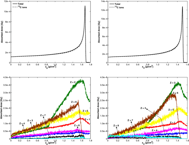
Figure 5. Numerical simulations of the absorbed dose distributions as a function of depth in graphite (left) or in water (right). The upper figures represent the total absorbed dose and the contribution of 12C ions. The lower figures provide the contribution of projectile fragments with different atomic numbers Z.
Download figure:
Standard image High-resolution image3.2. Fluence correction factors
A comparison of measured and calculated fluence correction factors is shown in figure 6. As shown in figures 6(A) and (B), the sensitivity of the results to small errors in depth scaling in the vicinity of the Bragg peak induces large fluctuations of the experimental fluence correction factors and the results are not conclusive in this region. Hence, the results in the vicinity of the Bragg peak will not be shown in the remaining figures. In all cases, the fluence correction factors increase with depth. There is a good match between the numerical and experimental results. The calculated fluence correction factors using GATE/Geant4 increase to about 0.5% or 0.25% above unity close to the Bragg peak depending on whether they are determined for the carbon ion spectrum only or for all charged particles. The values are consistent with the experimental results. Experimental data increase towards 1.01 before the Bragg peak. The two lower points, at 0.18 and 0.393 g cm−2, are probably due to an experimental issue noticed with the determination of the graphite ionization curve and they can be omitted. The issues observed at these small depths could be due to inhomogeneities in the graphite plates used, air gaps between the plates or possibly a plate alignment problem. The experimental behaviour is similar to that obtained for a clinical 60 MeV proton beam (Al-Sulaiti et al 2010). The average random uncertainty (type-A (JCGM 100: 2008)) derived from experimental data is around 0.25% (1 std. dev.). Four different numerical curves are represented in this figure. Solid squares and solid circles represent kfl, num based on the fluence approach represented by equation (2.7a), when taking into account either all the charged particles spectra (squares) or carbon ion spectrum only (circles). Solid triangles and solid stars show kfl, num based on the dose approach using equation (2.8a), i.e. based on stopping power and absorbed dose, considering all the charged particles spectra (stars) or carbon ions only (triangles). The step on the curves which shows the result for all the charged particles spectra, in zw-eq = 0.77 g cm−2, is due to the artefact mentioned above for alpha particles in Geant4. The stopping power values applied have been determined with the Geant4 class 'G4EMCalculator', which allows a direct access to fundamental electromagnetic quantities. Except for alpha particles at low energies, the obtained values for the stopping power of ions are close to recommended values in ICRU Report 49 and ICRU Report 73. The difference between Geant4 values and ICRU values is lower than 0.5% in water and 4% in graphite, except for alpha particles for which the difference increases up to 30% in water and 25% in graphite at low energy. Figure 7 shows the water-to-graphite electronic mass collision stopping power ratio. Using equations (2.5a) and (2.5b), two results are compared: the one based on ϕg and the other based on ϕw. Similar results are obtained for sw, g(ϕg) and sw, g(ϕw). The differences between these two values are smaller than 0.035%, justifying the equivalence of the stopping power ratios. According to equations (2.6), the consequence of this conclusion is the similarity of the behaviour between kfl, num and  , as observed in Palmans et al (2013a). Before the Bragg peak, the water-to-graphite stopping power ratio can be approximated by a constant value of 1.1146 ± 0.0001 for sw, g(ϕg) and 1.1144 ± 0.0001 for sw, g(ϕw) (only type-A uncertainty).
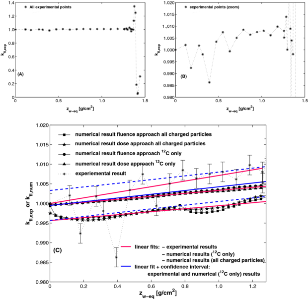
Figure 6. Numerical and experimental fluence correction factors for an 80 MeV/A carbon ion beam as a function of water-equivalent depth. (A) and (B) show the experimental data only and (C) shows a comparison of numerical and experimental results up to the Bragg peak region. In (C), solid circles and solid squares are based on the fluence approach of equation (2.7a), and solid triangles are based on the dose approach of equation (2.8a). The solid circles and solid triangles show results where only the carbon ion spectrum has been considered, while for the solid squares and the solid stars, all the charged particles spectra have been included.
Download figure:
Standard image High-resolution image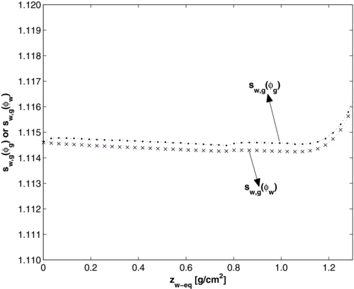
Figure 7. Numerical simulation of water-to-graphite electronic mass collision stopping power ratio as a function of water-equivalent depth, evaluated for graphite fluence spectra (dots) or water fluence spectra (crosses).
Download figure:
Standard image High-resolution imageWhen considering carbon ions only, the fluence correction factor is very close to unity at the surface and increases linearly with depth. However, when all particles are included in the result, a deviation from unity is observed at the surface, as has also been found by Lühr et al (2011) and Palmans et al (2013a). The fluence correction factor increases then with depth. The lower values observed in the numerical case of all charged particles are due to the absence of the ionization chamber in the numerical simulation. Indeed, the energy and the range of alpha particles are very low, so that these particles do not penetrate the wall of the ionization chamber and they do not influence the experimental fluence correction factor, unlike what is shown in figure 6(C). This result indicates that the ionization chamber induces perturbations and we should include it in our numerical analysis. As shown in figure 6(C), determined from the average of the results based on fluence approach and dose approach, fluence correction factors can be approximated by a linear fit. When considering only carbon ions, the latter is given by

When considering all the charged particle spectra, the linear fit is given by

When considering the experimental data (without data zw-eq = 0.180 g cm−2 and zw-eq = 0.393 g cm−2), the linear fit is given by

If all experimental data are included, then the linear fit is given by

When considering experimental and numerical data for carbon ions only, the linear fit is given by

The latter is shown in figure 6(C) with a confidence interval of 95%.
A comparison with the linear fit resulting from numerical simulations of a clinical 60 MeV proton beam (Palmans et al 2013a) shows that the slope of the fluence correction factor of an 80 MeV/A carbon ion beam is more than twice the slope of the fluence correction factor of a 60 MeV proton beam. At a depth of 0.6774 g cm−2, used for calorimetry measurements that will be described in a future publication, the fluence correction factor obtained with equation (3.5) equals 1.0027.
In order to investigate the influence of the LNS beam line configuration (cf figure 2) on the fluence correction factors, this quantity has been determined for an 80 MeV/A monoenergetic carbon ion beam in different configurations. Figure 8 illustrates the absorbed dose distributions, normalized to unity at the entrance, as a function of depth in water (upper) and graphite (lower) for three different configurations: (case 1) simulation of an 80 MeV/A carbon ion beam for the full LNS beam line, (case 2) simulation of an 80 MeV/A monoenergetic carbon ion beam in which the phantom is at the same position as for the previous simulation but in absence of the scatter foils, exit window and collimator (there is an air gap between the beam and the phantom of 189.1 cm) and (case 3) simulation of an 80 MeV/A monoenergetic carbon ion beam in which the beam source is at the phantom surface. CSDA range values are presented for each situation in table 1, in graphite and water. Both for graphite and water, there are differences of 1.1% and 14.5% between cases 1 and 2, and between cases 1 and 3, respectively. In graphite, these differences equal 0.0187 g cm−2 between cases 1 and 2, and 0.2435 g cm−2 between cases 1 and 3. In water, these differences equal 0.0168 g cm−2 between cases 1 and 2, and 0.2185 g cm−2 between cases 1 and 3. These values correspond with the water- or graphite-equivalent thickness of the exit window and the camera monitor in the first comparison, or the air column in the second comparison. The graphite-to-water ratio of these values equals the water-to-graphite stopping power ratio, i.e. 1.1145. The range in case 2 corresponds to a 74.625 MeV/A carbon ion beam in case 3.

Figure 8. Influence of the LNS beam line and the air gap on the absorbed dose distribution. Comparison for an 80 MeV/A carbon ion beam between three situations: LNS beam line—case 1 (continuous line), a monoenergetic beam with an air gap between the beam and the phantom—case 2 (dashed line) and a monoenergetic beam without air gap between the beam and the phantom—case 3 (dot–dashed line). All results are presented as a function of depth in water (upper figure) or in graphite (lower figure) and they are normalized to 1 at the entrance.
Download figure:
Standard image High-resolution imageTable 1. Range of an 80 MeV/A carbon ion beam in graphite and water for three different situations: the LNS beam line (case 1) and a monoenergetic carbon ion beam (cases 2 and 3).
| Range in graphite (g cm−2) | Range in water (g cm−2) | |
|---|---|---|
| Case 1 | 1.6830 | 1.5079 |
| Case 2 | 1.7017 | 1.5246 |
| Case 3 | 1.9265 | 1.7264 |
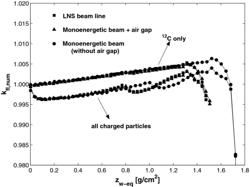
For each case, figure 9 shows two plots of the fluence correction factors as a function of the water-equivalent depth: if the carbon ion spectrum is considered alone or if all the charged particle spectra are included. Results are based on equation (2.7a). The behaviour of the fluence correction factors is similar in all cases, with that the same shift is observed for depth dose in water presented in figure 8, i.e. 0.2185 g cm−2 between cases 1 and 3, and 0.016 78 g cm−2 between cases 1 and 2.
Figure 9. Comparison of the numerical fluence correction factors determined with Geant4/GATE and based on equation (2.7a). Comparison between three situations (the same as those presented in figure 8: the INFN-LNS transport beam line (solid squares) and an 80 MeV/A monoenergetic carbon ion beam (case 2: solid triangles and case 3: solid circles). For all situations, two different cases are illustrated: the case where only the carbon ion spectrum is considered and the case in which all charged particle spectra are included.
Download figure:
Standard image High-resolution image
4. Conclusions
Fluence correction factors to correct the conversion from dose-to-graphite in a graphite phantom to dose-to-water in a water phantom for an 80 MeV/A carbon ion beam are presented in this work. This study has been performed in view of establishing a graphite calorimeter as a primary standard to determine the absorbed dose-to-water in therapeutic beams. Indeed, as specified in the IAEA dosimetric protocol, the absorbed dose has to be established in water. For practical reasons, a new portable graphite calorimeter has been developed at NPL, and that will be used in future work to determine an experimental value of the mean energy expended in air per ion pair formed, wair-value, for an 80 MeV/A carbon ion beam. Since using a graphite calorimeter, results are obtained in graphite, the conversion between absorbed dose-to-graphite and absorbed dose-to-water, which depends on the water-to-graphite mass collision stopping power ratio and fluence correction factors, was investigated here.
The main result of this study is the experimental and numerical determination of fluence correction factors. Except at the phantom surface, the agreement between the measured data and calculated values is satisfactory. If only the carbon ion spectrum is considered, then both numerical and experimental fluence correction factors increase slowly above unity up to the Bragg peak. kfl, num and kfl, exp increase by about 0.5% and 1% respectively. Numerical values have been derived by two different methods, using equation (2.7a) or (2.7b). Similar results are obtained with both methods. If all the charged particles spectra have been included, due to the influence of alpha particles, then the fluence correction factors values are below unity at the surface and increase up to 1.025 before the Bragg peak. The lower values observed for the curve of all charged particles indicate that the ionization chamber induces perturbations that we should include in the analysis. Taking into account the numerical and experimental data, the fluence correction factor can be approximated by linear fit as a function of the water-equivalent depth: kfl, all = 0.9995 + 0.0048 zw-eq.
The second contribution to the absorbed dose conversion, i.e. the electronic mass collision stopping power ratio, is shown larger than the fluence correction factors. For an 80 MeV/A carbon ion beam, the water-to-graphite electronic mass collision stopping power ratio equals 1.115.
In conclusion, it has been shown that using experimental and numerical results presented in this paper, a graphite calorimeter can be used in a clinical carbon ion beam to determine the absorbed dose-to-water, as recommended by practical dosimetric protocols to be used in clinical dosimetry. This conversion increases linearly with depth between 1.115 at the entrance and 1.118 at zw-eq = 0.76 g cm−2. This work is part of a large study with the aim to develop a graphite calorimeter for light-ion beams.
Acknowledgments
This work is supported by the BioWin program of the Walloon Government in Belgium. The authors acknowledge the Acoustics and Ionising Radiation Metrology Programme of the National Measurement System, UK and the EMRP joint research project MetrExtRT which has received funding from the European Union on the basis of Decision No 912/2009/EC. The EMRP is jointly funded by the EMRP participating countries within EURAMET and the European Union.
Footnotes
- 6
- 7
- 8
Ion Beam Application (IBA), Avenue Baudouin 1er 25, 1348 Ottignies-Louvain-la-Neuve—IBA dosimetry: www.iba-dosimetry.com
- 9
- 10
- 11