


ABSTRACT
We present the first 3D whole-prominence fine structure model. The model combines a 3D magnetic field configuration of an entire prominence obtained from nonlinear force-free field simulations, with a detailed description of the prominence plasma. The plasma is located in magnetic dips in hydrostatic equilibrium and is distributed along multiple fine structures within the 3D magnetic model. Through the use of a novel radiative transfer visualization technique for the Hα line such plasma-loaded magnetic field model produces synthetic images of the modeled prominence comparable with high-resolution observations. This allows us for the first time to use a single technique to consistently study, in both emission on the limb and absorption against the solar disk, the fine structures of prominences/filaments produced by a magnetic field model.
Export citation and abstract BibTeX RIS
1. INTRODUCTION
In this paper we present the first 3D whole-prominence fine structure (WPFS) model. The model combines together 3D simulations of the magnetic field configuration of an entire prominence, with a detailed description of the prominence plasma. In the WPFS model the prominence plasma is distributed along multiple fine structures located in magnetic dips. The plasma properties in each dip depend on the local magnetic field configuration.
Over the last two decades many authors have developed 3D models simulating the entire magnetic field structure of solar prominences. Most of these models produce magnetic field configurations containing magnetic dips that can accommodate the prominence plasma and support it against gravity. These models can be divided into two groups, static and dynamic. Static models construct either individual magnetic field configurations or sequences of independent configurations without a direct evolution between them (Mackay et al. 1997, 1999; Aulanier & Démoulin 1998; Aulanier et al. 1999, 2000; Régnier & Amari 2004; van Ballegooijen 2004; Dudík et al. 2008, 2012; Gunár et al. 2014). Dynamic models, on the other hand, produce magnetic field configurations by evolving an initial configuration over consecutive time steps (van Ballegooijen & Martens 1989; Galsgaard & Longbottom 1999; DeVore & Antiochos 2000; Martens & Zwaan 2001; Lionello et al. 2002; Mackay & Gaizauskas 2003; Mackay & van Ballegooijen 2005, 2006, 2009; Xia et al. 2011, 2012). More details on the prominence magnetic field models can be found in the review by Mackay et al. (2010).
In this paper we use the 3D magnetic field configuration of an entire prominence, produced by the 3D nonlinear force-free field (NLFF) simulations of Mackay & van Ballegooijen (2009). These authors consider a time sequence of related static field configurations produced by advecting a single magnetic bipole toward the main body of a filament.
To obtain a realistic distribution of the plasma in the prominence fine structures, two techniques can be used. It can be obtained from considering an equilibrium with the local magnetic field configuration or, alternatively, by simulating the physical processes responsible for the prominence formation.
Luna et al. (2012) developed a model for the formation and evolution of prominence fine structures based on the 3D double sheared arcade simulations of the whole-prominence magnetic field of DeVore et al. (2005). Individual prominence fine structures are formed dynamically using the 1D thermal non-equilibrium models of Karpen et al. (2006). Luna et al. (2012) have shown that the modeled signatures of moving prominence fine structures, such as the thermal properties, velocity, and mass, are in many ways consistent with the observations of the Atmospheric Imaging Assembly (AIA; Lemen et al. 2012) on board the Solar Dynamics Observatory (SDO). However, we note that the so-called Hα-proxy channel (Karpen et al. 2001), used for example by Luna et al. (2012) to visualize the locations of colder plasma (around 30,000 K in their case), is not directly comparable with the Hα visualization technique used in this paper.
The 2D magnetohydrostatic equilibrium of Kippenhahn–Schlüter type (Kippenhahn & Schlüter 1957) was used by Heinzel & Anzer (2001) to construct a 2D gravity-induced model of vertical prominence fine structures. The prominence plasma distributed inside the resulting magnetic dips has a temperature structure described semi-empirically to accommodate the prominence–corona transition region (PCTR). Heinzel & Anzer (2001), and later Heinzel et al. (2005), and Gunár et al. (2007a) showed that such individual prominence fine-structure threads can produce realistic synthetic hydrogen spectra, including the Lyman line series, Lyman continuum, and the Hα line. Moreover, as was demonstrated by Gunár et al. (2007b, 2008, 2010), and more recently by Berlicki et al. (2011) and Gunár et al. (2011, 2012), the synthetic spectra obtained from a random spatial distribution of multiple 2D threads are in good agreement with the spectral observations of quiescent prominences.
Recently, Gunár et al. (2013a) used magnetic dips produced by the NLFF simulations of Mackay & van Ballegooijen (2009) as the local magnetic field configuration instead of the gravity-induced dips of Heinzel & Anzer (2001). These authors developed a novel iterative technique for filling magnetic dips with prominence plasma in hydrostatic equilibrium. They used a semi-empirical temperature structure that includes the PCTR, similar to that used by Heinzel & Anzer (2001). Gunár et al. (2013a) also used 2D non-LTE radiative transfer modeling to show that such prominence fine structures can produce synthetic hydrogen spectra in agreement with observations. In the present paper we use the iterative method of Gunár et al. (2013a) to fill an entire set of dips of a simulated prominence with plasma to produce multiple individual fine structures.
A detailed description of prominence physics can be found in textbooks such as Tandberg-Hanssen (1995) or Vial & Engvold (2015), and in reviews by Labrosse et al. (2010) and Mackay et al. (2010). The specific properties of the prominence fine structures were reviewed by Heinzel (2007), their modeling by Gunár (2014), and their observational characteristics by Parenti (2014).
In this paper we aim to put forward a new prominence modeling technique which we develop using the magnetic field configuration produced by simulations of Mackay & van Ballegooijen (2009). In the future this technique may be applied to a wide range of prominence magnetic field models. Here we do not attempt to compare the results of the WPFS modeling with any particular observed prominences. Such a study will be considered later. Rather, we aim to show that this technique produces prominence images that are in principle in agreement with non-eruptive solar prominences. To this end we make use of the newly developed method of Heinzel et al. (2015) that allows us to visualize the 3D WPFS model in the Hα line by performing fast 1D radiative transfer calculations along a large number of line of sight (LOS). Using such a visualization technique we are able to produce self-consistent synthetic Hα images of the plasma loaded magnetic field model, viewed both as a prominence on the limb and also as a filament, in absorption against the solar disk.
In Section 2 we describe the general scheme for producing a WPFS model. Details of the first combined whole-prominence magnetic field and fine-structure plasma model are given in Section 3. In Section 4 we provide a short description of the hydrogen Hα line visualization method and show synthetic images from the model. Section 5 contains the discussion and Section 6 provides our conclusions.
2. SCHEME FOR A GENERAL WPFS MODEL
In this section we highlight the main stages in the construction of a general WPFS model (for illustration see Figure 1). These are not specific to any magnetic model and can be applied to other prominence models based on different magnetic field simulations.
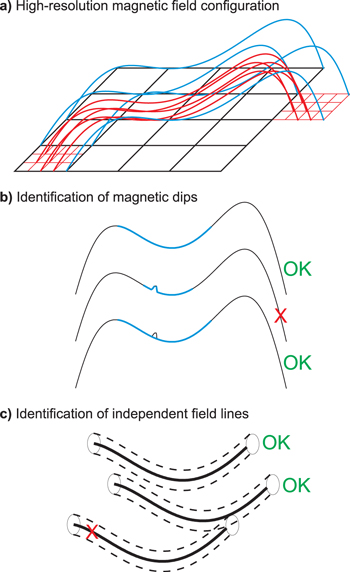
Figure 1. Schematic drawings illustrating individual stages of a general WPFS model construction: (a) high-resolution magnetic field configuration, (b) identification of magnetic dips, and (c) identification of independent field lines.
Download figure:
Standard image High-resolution image2.1. High-resolution Magnetic Field Configuration
Any simulated prominence magnetic field configuration intended for use in WPFS modeling has to have sufficiently high resolution (Figure 1(a)). This is needed to allow the WPFS model to naturally resolve the internal structure of the modeled prominence without creating any numerical artifacts, such as grid-dependent features. Such artifacts could be layers of dips at the same height with gaps in between them. This can be caused by tracing field lines only from sparsely distributed grid points. The level of the required resolution (density of points from which field lines are traced) is related to the dimensions of the assumed cross-section of the individual prominence plasma fine structures. For example, the size of the gaps of unresolved magnetic field lines between layers of (resolved) dips must be smaller than the cross-section of the plasma fine structures. We note that such a relation is strongly dependent on the nature of the prominence magnetic field configuration used and should be considered individually for various WPFS models.
2.2. Identification of Magnetic Dips
Special attention needs to be paid to the identification of the dipped portions of magnetic field lines (Figure 1(b)). An automatic procedure identifying all of the dips within a magnetic field configuration may recognize series of very small dips located along a single field line inside a much large dip but not take into account the presence of the large dip itself. Because the large and deep dips have a much greater impact on the internal structure of the prominence than smaller shallow ones (they can hold significantly more dense mass and thus be much more visible), they need to be all properly identified. In the case where small dips are identified within a much larger dip, a small hump of the magnetic field should be removed (see Figure 1(b)).
2.3. Identification of Independent Field Lines
High resolution magnetic field configurations result in a large number of often densely packed field lines with their respective minimum distances less then the assumed cross-field dimensions of the prominence plasma fine structures. As any overlap between prominence plasma fine structures needs to be avoided (for numerical reasons), only field lines that are at a given distance from all other selected field lines are to be chosen (Figure 1(c)). The given distance is based upon the chosen cross-section of the plasma fine structures. In this work we call such field lines independent. To ensure that no arbitrary selection criteria will influence the appearance of the modeled prominence, a random selection process can be used to find all independent field lines.
2.4. Filling Magnetic Dips with Prominence Plasma
In the case where the configuration of the magnetic field is not varying significantly on the spatial scales comparable with the assumed cross-section width of the prominence plasma fine structures, one can use a selected field line as a representation of the shape of the magnetic field inside the whole cross-section. The dipped portion of such a field line can be filled with prominence plasma, for example, by a plasma in hydrostatic equilibrium using the method developed by Gunár et al. (2013a). This provides the variation of the plasma parameters along the field line. Next, a realistic plasma distribution within the cross-section can be assumed to derive a full 3D description of the plasma forming individual prominence fine structures. In this way all independent field lines can be filled with prominence plasma. Each of the resulting prominence fine structures will depend on the shape of the dipped portion of its respective guiding field line and thus will be composed of plasma influenced by the local configuration of the whole-prominence magnetic field.
3. COMBINED 3D WHOLE-PROMINENCE MAGNETIC FIELD AND PLASMA MODEL
3.1. Whole-prominence Magnetic Field Model
We use the results of the 3D NLFF simulations of Mackay & van Ballegooijen (2009) as a realistic prominence magnetic field configuration. However, it is not our intention to validate these simulations by comparing them with other models or observations. We use them as the starting point for the development of the fine structure models of entire prominences. In these simulations the initial distribution of the magnetic flux in the photosphere was chosen to be that of a magnetic arcade, but with flux concentrations that are displaced from one-another. One unit in the dimensionless length-scale is chosen to be 60,000 km, with the arcades separated by two length-scale units, i.e., 120,000 km. These choices are arbitrary but are taken such that the arcades lie four typical supergranular cells apart. The initial flux distribution in the photosphere is shown in Figure 2(a). The solid/dashed contours denote positive/negative flux. From this photospheric distribution we construct a 3D linear force-free field with the value of α fixed at  m−1. This is sufficiently large to produce a dipped magnetic field configuration representing the basic structure of a prominence. This linear force free field is used as the initial condition. We note that the chosen value of α is well below the critical value, which is −2.14 × 10⁻⁸ m−1.
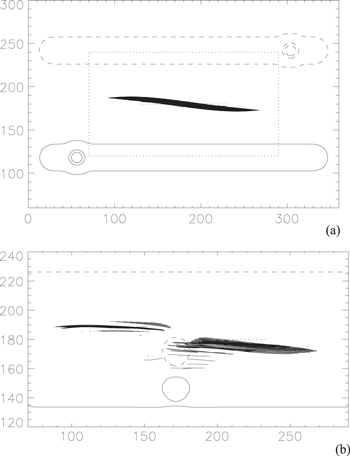
Figure 2. (a) Initial condition of the NLFF prominence magnetic field simulations. Dipped portions of the field lines are drawn (bold lines) up to the depth of one PSH. The solid/dashed contours represent positive/negative values of Bz at levels of ±70, ±50, ±1 Gauss. (b) Enlarged view of the area highlighted by the dotted box in the panel (a). Filament is shown after 3000, 60 s time-steps after the insertion of the bipole. Dimensions are in 103 km.
Download figure:
Standard image High-resolution imageTo detect the presence of magnetic dips in the resulting configuration, each grid point within the 3D computational domain is tested. Dips occur when the vertical component of the field satisfies

All grid points satisfying this criterion are used as the starting points for plotting magnetic field lines.
In Figure 2 portions of dips are drawn up to the depth of one pressure scale-height (PSH) or until the height of the lower peak is reached. For the case of an isothermal plasma and assuming a temperature of 10,000 K, the dip depth equal to one PSH is approximately 300 km. We note that this technique, commonly employed in simulations of the prominence magnetic field, is not used elsewhere in this work, apart from Figure 2.
After the initial magnetic flux distribution is established a bipole is inserted into the initial configuration through the technique described in Section 2.2.3 of Mackay & van Ballegooijen (2009). The bipole is placed in the positive polarity side of the polarity-inversion line (PIL) and is aligned parallel to the overlying arcade as can be seen in Figure 2(b). The ratio of bipole flux ( ) to arcade flux (
 ) is
) is  , while the ratio of bipole to filament flux (
 ) is
) is  . With this orientation the minority polarity for this side of the PIL lies closest to the dips and is then advected toward the main body of the filament by a boundary flow. As the minority polarity is advected toward the main body of the filament, the coronal field is perturbed and evolves through a series of quasi-static NLFF states as described by the magneto-frictional technique of van Ballegooijen et al. (2000) and Mackay & van Ballegooijen (2006). In Figure 2(b) we show an enlarged view of the filament after 3000, 60 s time-steps. Due to the presence of the bipole the main body of the filament separates into two parts. The gap between them is caused by the absence of dips, not an absence of plotted field lines. Full details of the 3D NLFF prominence magnetic field simulations can be found in Mackay & van Ballegooijen (2009).
In this paper we use the simulation snapshot after 2000, 60 s time steps (similar to Figure 2(b)) as the 3D magnetic field configuration of the WPFS model. To obtain a magnetic field resolution that is sufficiently high to resolve prominence plasma fine structures with cross-section width of 1000 km, we increased the original resolution of the grid used in the NLFF simulations from 2563 to 12803 grid points. In such a high-resolution configuration we identify nearly 40,000 dipped field lines. For selection of those field lines that can accommodate non-overlapping plasma fine structures we use multiple randomizations that help us to overcome any arbitrary selection effects. We randomly select the first field line to be taken as independent and then we scan through all other dipped field lines in a random order. The minimum distance of the dipped portion of each scanned field line is evaluated against all field lines already found to be independent. If the minimum distance is above the assumed cross-section width of the prominence plasma fine structures (in this case 1000 km), the scanned field line is also taken to be independent. Then the next field line (in random order) is considered, until all dipped field lines in the magnetic field configuration are scanned. The total number and composition of a set of independent field lines depends on the random choice of the starting field line and on the random order of the subsequently scanned field lines. In Figure 3 we show the configuration of 835 independent field lines (out of about 40,000) in the top view (x–y plane) and side views (x–z and y–z planes). Only dipped portions that will be filled with prominence plasma (see next section) are plotted.
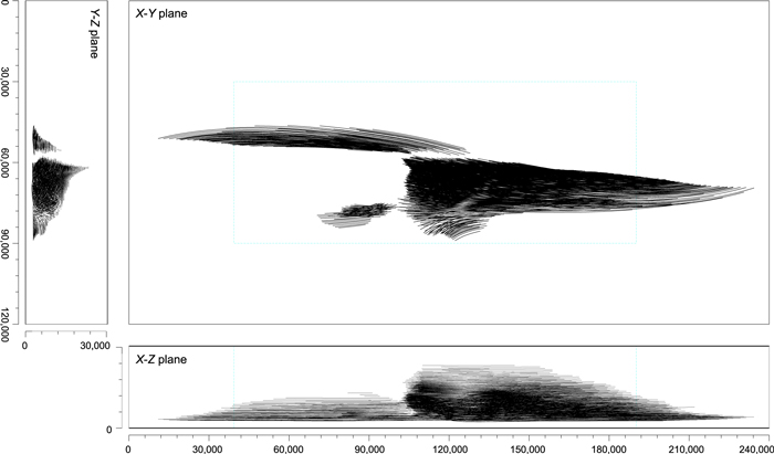
Figure 3. Whole-prominence magnetic field configuration with 835 independent field lines plotted in the top view (x–y plane) and side views (x–z and y–z planes). Only dipped portions filled with prominence plasma are drawn. Dimensions are in km.
Download figure:
Standard image High-resolution image3.2. Prominence Fine Structure Plasma
To obtain the plasma distribution within the entire prominence we fill the dipped portions of all (or a randomly selected part of) the independent field lines with plasma in hydrostatic equilibrium using the method developed by Gunár et al. (2013a). This was shown to produce individual prominence fine structures with a realistic distribution of the gas pressure and temperature including the PCTR.
In this work we use a special 3D grid on which we define all physical quantities of all fine structures. The choice of this grid is based on the fact that all dips in the magnetic field configuration used are preferably oriented along the x-axis of our computational domain. This allows us to use less dense spacing along the x-axis (along the length of the dips) and a denser spacing only in the y–z plane (see Figure 4). We further assume that cross-sections of all prominence fine structures are parallel to the y–z plane instead of being strictly perpendicular to the local magnetic field vector. This allows us to significantly simplify the development of this first 3D WPFS model and ease the computational demands. However, a general WPFS model will require dense spacing in all three-dimensions. In this work we use a grid spacing of 10 km in the y–z plane and 150 km along the x-axis for the plasma distribution.
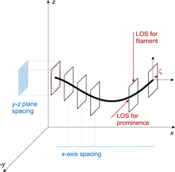
Figure 4. Drawing illustrating the spacing along each axis and the LOS directions used for visualization of the model as a prominence and a filament.
Download figure:
Standard image High-resolution imageEach magnetic dip is filled iteratively from its bottom until it either reaches the required column mass, or until the height of the lower shoulder of the dip is reached. The temperature variation of the plasma inside the dip is prescribed semi-empirically and considers two distinct shapes of the PCTR. These represent a steep gradient of the temperature in the direction perpendicular to the magnetic field and a more gradual temperature increase in the direction along the field. The temperature variation along the field is defined for the left and right part of the dip individually as

Here ξ represents the geometrical coordinate parallel to x, but defined from the center of the local dip toward either its left or right edge. T0 is the central minimum temperature and  represents the transition region temperature. The temperature gradient along the magnetic field lines is described by the exponent
  . This formula is based on the temperature variation used by Heinzel & Anzer (2001). The exponent
  considers the effect of the thermal conductivity along the magnetic field lines resulting in a gradual rise of the temperature from the cool central part toward the PCTR. In this work, we use values of T0 = 7,000 K, Ttr = 100,000 K, and
  for all prominence plasma fine structures (see Table 1).
Table 1. List of Parameters Identical for All Fine Structures in this Work
| Par. | Description | Value |
|---|---|---|
| T0 | Central minimum temperature | 7,000 K |
| Ttr | Transition-region temperature at the edge of a dip | 100,000 K |
| M0 | Maximum column density in the middle of the thread | 1 × 10⁻⁴ g cm−2 |
| ptr | Transition-region gas pressure at the edge of a dip | 0.015 dyn cm−2 |
| γal | Exponent describing temperature gradient along the field | 2 |
| γac | Exponent describing temperature gradient across the field | 60 |
| ic | Ionization degree at the dip center | 0.3 |
| AHe | Helium-to-hydrogen abundance ratio | 0.1 |
| 2δ | Cross-section width of prominence fine structures | 1000 km |
Download table as: ASCIITypeset image
The hydrogen ionization degree i is estimated using the equation

adapted by Gunár et al. (2013a) from Heinzel & Anzer (2001). The parameter  represents the estimated degree of ionization at the dip center, as suggested by Anzer & Heinzel (1999). The mean molecular mass μ of a hydrogen–helium plasma is given by

where  is the helium-to-hydrogen abundance ratio.
To obtain the gas pressure variation along the central field line we define the transition region pressure  at both edges of the local dip and then evaluate an integral of the form

over the depth z-coordinate from both edges toward the bottom of the dip over the local total depth Z. Here,  is the mass of the hydrogen atom and g is the gravitational acceleration at the solar surface. For all prominence fine structures we assume that the transition region gas pressure
  is equal to 0.015 dyn cm−2. This corresponds to the prominence boundary values listed e.g., by Engvold et al. (1990; see also Labrosse et al. 2010), and is consistent with our previous work. To obtain the column mass we integrate the density in the local dip along the ξ-coordinate.
After we specify the plasma distribution along the guiding field line we next need to define the variation of all physical quantities within the fine structure cross-section. We assume that the magnetic field does not change considerably on the scale of the cross-section width and thus we use a uniform dipped magnetic field within an individual prominence plasma fine structure. For simplicity we set the geometrical cross-section planes to be parallel to the y–z plane. Furthermore we do not assume any physical mechanism influencing the plasma distribution within the fine structure cross-section, but we use an angularly symmetric distribution, resulting in the de facto circular cross-section. We describe it in Cartesian coordinates within the y–z plane on a grid of 101 × 101 equidistantly spaced grid points. This gives us a resolution of 10 km when we assume the cross-section width of 1000 km. Such fine spacing is necessary to resolve the steep temperature gradient in the direction perpendicular to the magnetic field lines. Such a grid is defined locally at each x position along each field line and is always centered at the guiding field line. The cross-section width of 1000 km assumed here is consistent with the 2D models of Heinzel & Anzer (2001). However, we note that observations of filaments in the hydrogen Hα line, such as those of Lin et al. (2005), indicate that the fine structure widths in some filaments may be as small as 100 km.
The temperature variation within the fine structure cross-section in the center of the dip is defined as

where  km (total cross-section dimension is 2
  km). Here ζ represents the geometrical coordinate parallel to y, but defined from the center of the fine structure cross-section. The exponent
  describes the steep temperature gradient across the field. Here we use
  . Such a steep gradient reflects the effect of the inhibited thermal conductivity in the direction across the magnetic field.
To obtain the gas pressure and density variation across the field lines, we specify the variation of the column mass in the center of the dip in the cross-field direction as

Thus at the given y-position  is used as the required column mass and
  is used as the minimum temperature at the bottom of the dip.
The values of the parameters that are fixed for every fine structure in the WPFS model are listed in Table 1. The current values are consistent with the work of Gunár et al. (2013a). We discuss the possible effects of varying these parameters in Section 5.
4. Hα VISUALIZATION
Once we have the 3D model of the whole prominence with a detailed description of its plasma located in multiple fine structures, we can use the novel approximate radiative transfer method of Heinzel et al. (2015) to obtain the synthetic Hα spectra. This allows us to perform fast 1D radiative transfer calculations in the Hα line along any given LOS, without the need for multi-level, multi-dimensional radiative transfer modeling. The obtained synthetic Hα spectra are reasonably accurate in case the individual fine structures have optical thickness below unity (see Heinzel et al. 2015). Although such synthetic Hα spectra might not be useful for direct comparison with the radiometrically calibrated spectral observations (where multi-level and multi-dimensional radiative transfer modeling is essential), it can be used for visualization of the 3D WPFS models. For this purpose synthetic Hα intensity can be integrated in a narrow spectral region to obtain intensities comparable with the narrow-band filtergrams, such as those obtained using the Narrowband Filter Imager of the Solar Optical Telescope (SOT, Tsuneta et al. 2008) on board Hinode (Kosugi et al. 2007). In the following paragraph we give a short description of this method; details can be found in Heinzel et al. (2015).
4.1. Hα Synthesis Method
To obtain the Hα intensity along a given LOS we assume a uniform Hα line source function S in the whole medium (see Section 2.1 of Heinzel et al. 2015). This reduces the radiative transfer equation to the well-known form

where

The term d
 is the optical-depth increment corresponding to the geometrical path increment dl along the given LOS and
  is the absorption coefficient for the Hα line.
  is the total optical thickness along the LOS, integrated through all structures crossed by the given LOS. The absorption coefficient
  has the standard form (Heinzel et al. 2015)
where f23 is the Hα line oscillator strength, n2 the hydrogen second-level population, and  is the normalized line profile. Since we can assume that the individual fine structures have a low optical thickness, the normalized line profile is a Gaussian with dependence on the thermal and micro-turbulent broadening. In this work we use a uniform micro-turbulent velocity of 5 km s−1 (see e.g., Engvold et al. 1990; Labrosse et al. 2010). To estimate n2 we use the relation between the electron density
  and n2

discussed in Heinzel et al. (2015); see also Heinzel et al. (1994). The electron density can be estimated from the local values of gas pressure and temperature provided by the WPFS model using the well known formula (Heinzel et al. 2015)

and assuming 10% abundance of helium and no helium ionization. Values for the factor f and the hydrogen ionization degree i, together with the source function, are tabulated in Heinzel et al. (2015) for various values of temperature, gas pressure, and altitude above the solar surface.
4.2. Prominence Visualization
To visualize our WPFS model as a prominence, i.e., in emission above the solar limb without any background radiation, we use the LOS oriented perpendicular to the x–z plane (parallel to the y-axis). This is consistent with the x–z plane view in Figure 3. To obtain the synthetic images we construct a grid with 150 × 150 km spacing covering the x–z plane. This results in a synthetic resolution comparable with the Hinode/SOT Hα observations.
We evaluate Equation (8) at each grid point along the LOS parallel to the y-axis taking into account the local distribution of temperature and gas pressure in any prominence plasma fine structure intersected by the given LOS. For simplicity and to save computational resources we assume an altitude of 10,000 km above the solar surface in the whole model. We also assume representative values of f and i instead of interpolating these values from the tables in Heinzel et al. (2015). While such simplification introduces a certain inaccuracy, it is sufficiently precise for the purpose of this paper. For an altitude of 10,000 km we use tabulated values for T = 8000 K and  dyn cm−2 giving
  and i = 0.44. We also at this stage evaluate Equation (8) only at the frequency of the Hα line center.
In Section 3.1 we identified a set of independent field lines that produce non-overlapping prominence fine structures. However, not all of these field lines have to necessarily contain prominence plasma. To illustrate the effect of the so-called filling factor—ratio of the volume filled by prominence mass to the total volume taken up by a prominence—we use three different scenarios. We either fill all independent field lines, or we randomly select 25% or 50% of the field lines to be filled. In Figure 5 we plot for each of these cases the synthetic Hα line center image in emission (in color) and also as a negative image to ensure a better visibility of the plotted prominence fine structures. The body of the modeled prominence is broken-up into two parts, similar to the results of Mackay & van Ballegooijen (2009); see Figure 2. The left detached part of the prominence is considerably fainter than the right part and the gap between them appears much larger than that seen in the plot of the dipped portions of the magnetic field lines in Figure 3. From the image it is clear that there is a significant amount of fine structures produced by the dips in the model. These fine structures show a predominantly horizontal pattern. However, as the number of filled field lines increases, some thin vertical structures also become visible. We note that most of the bright fine structures are located between roughly 120,000 and 140,000 km marks on the x-axis. This is where the majority of the deep dips are present. For an interested reader we recommend enlarging Figure 3 in the electronic format to distinguish these deep dips.
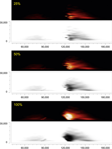
Figure 5. Synthetic Hα line center images of the WPFS model seen as a prominence for 25%, 50%, and 100% of filled independent field lines. Top panels of each pair show synthetic image in emission in color. Bottom panels show a negative image. Dimensions are given in km. The field of view corresponds to a segment marked in Figure 3.
Download figure:
Standard image High-resolution image4.3. Filament Visualization
To obtain the synthetic Hα image of our WPFS model as a (dark) filament seen in absorption against the bright solar disk, we use the LOS oriented downward in a direction perpendicular to the x–y plane (parallel to the z-axis). This is consistent with the x–y plane view in Figure 3. We again construct a grid with 150 × 150 km spacing, now covering the x–y plane. In filament visualization we have to take into account the background intensity from the solar disk that is absorbed by the prominence plasma. The total intensity emerging at the top of the prominence/filament structure is then given by the formula

The background intensity  in the Hα line center can be obtained, e.g., from David (1961).
In Figure 6 we show the synthetic Hα line center images of the WPFS model, seen as a filament (top panels of each pair) and a prominence (bottom panels), where 25%, 50%, and 100% of independent field lines are filled. Top panels show the filament synthetic image in absorption (not as a negative). Bottom panels show the prominence as a negative image. From this figure it can be seen that the bright prominence fine structures pile-up one above each other with seemingly random horizontal shifts. In contrast, when viewed as a filament they appear aligned and resemble ensembles of fibrils forming the structure of observed filaments. Note that the filament fine structures in the synthetic Hα images of our WPFS model are wider than those seen in observations. In observations they appear to have widths as small as 100 km (Lin et al. 2005).
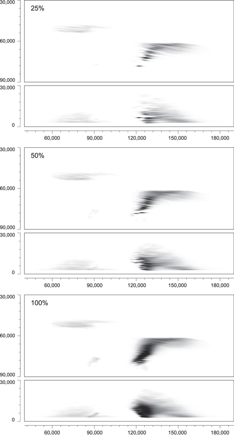
Figure 6. Synthetic Hα line center images of the WPFS model seen as a filament (top panels of each pair) and a prominence (bottom panels) for 25%, 50%, and 100% of filled independent field lines. Top panels show the filament synthetic image in absorption (not as a negative). Bottom panels show the prominence negative image. Dimensions are given in km. The field of view corresponds to a segment marked in Figure 3.
Download figure:
Standard image High-resolution image4.4. Calibration
For the visualization of the WPFS model and for a casual comparison with the Hα prominence/filament observations, it is sufficient to produce synthetic images in the Hα line center, such as those in Figures 5 and 6. However, for a qualitative comparison of a prominence model derived to reproduce observations of a specific prominence, one would need to pay attention to the consistency of the calibrations of the synthetic and observed images. First, case-specific values of the background Hα intensity would be needed and the uniformity of the source function should be properly justified. Values of the source function, together with the f and i values, could also be interpolated in altitude using the tables from Heinzel et al. (2015). Second, the resulting Hα intensity in each synthetic pixel should be an integral over a part of the synthetic Hα line profile corresponding to the bandwidth of the filter used for observations. Third, the sensitivity of the detector and the contrast of the observed images has to be considered and the same image properties applied to the synthetic filtergrams.
5. DISCUSSION
The WPFS model presented here allows us to study the fine structures of modeled prominences in a more realistic way than what is possible by the commonly used field line visualization techniques. These use simplified representations of the position and dimensions of the magnetic dips by plotting line segments. Their lengths correspond to the portion of the dip filled to a dip depth of one PSH, typically 300 km when assuming an isothermal plasma with a temperature of 10,000 K. Each dipped field line is plotted and the number and the density of visualized dips is dependent only on the number and density of grid points within the 3D computational domain. The number of field lines plotted is typically much lower than the high-resolution grid used here; see Section 3.1. Although this simplified method is often used as a representation of the Hα line visibility, it does not take into account any radiative transfer effects. The field line visualization technique thus leads to an exaggeration in the number of truly observable fine structures and at the same time it underestimates the dimensions of the strongly visible deep dips. This is due to the fact that the shallow dips, even if rather extended, can only contain hydrostatic plasma with low gas pressure. Such shallow dips result in a barely observable Hα emission. Higher Hα intensity comparable to the observed bright prominence fine structures can only be produced in sufficiently deep dips. These, on other hand, tend to be shorter and thus are drawn as shorter lines; see also discussion in Gunár et al. (2013a) and Gunár (2014).
This effect can be seen for example in Figure 5. Here bright localized structures (best seen in the 25% filled model) represent the emission of the denser prominence plasma located inside the deeper and shorter dips, i.e., dips with a small radius of curvature. Their higher density is caused by the higher gas pressure of the hydrostatic plasma due to their larger depth. These dips are equivalent to the Deep_dip described in Gunár et al. (2013a). The more dispersed Hα emission visible in Figure 5 originates in the shallower dips that tend to be more elongated and are similar to the Shallow_dip from Gunár et al. (2013a). The Hα emission from regions of shallower dips becomes stronger only due to integration through an increasing number of dips, which is well documented in Figure 5 with the increase of the filling factor. Because the Hα intensity decreases with the increase of the radius of curvature of the dipped magnetic field (and thus with the decrease of the central gas pressure) nearly flat dips become unobservable.
This fact is illustrated in Figure 7, which shows an example of the optical thickness in the Hα line center of the model with 50% field lines filled. Large areas filled with shallow dips (dips with large radius of curvature), e.g., in the left part of the prominence, have an optical thickness significantly lower than one.

Figure 7. Optical thickness in the Hα line center of the WPFS model with 50% filled field lines. Top panel shows model as a filament, bottom panel as a prominence. Dimensions are given in km. The field of view corresponds to a segment marked in Figure 3.
Download figure:
Standard image High-resolution image
The synthetic Hα line center images shown in Figure 5 resemble some high-resolution prominence Hα observations. However, the prominence fine structures shown in them are rather elongated and horizontally oriented, although vertical pile-ups of mostly bright features are also apparent. Therefore, these synthetic images do not correspond to the typical quiescent prominences dominated by multiple quasi-vertical fine structures, such as those studied by, e.g., Berger et al. (2008, 2010), Schmieder et al. (2010), and Gunár et al. (2012, 2014). On the other hand, they are more representative of prominences dominated by diffuse horizontal fine structures that are often associated with active regions (but are not eruptive) such as those studied by e.g., Okamoto et al. (2007); see also reviews of Patsourakos & Vial (2002) and Mackay et al. (2010). Interestingly, the 3D NLFF prominence magnetic field simulations of Mackay & van Ballegooijen (2009) used here were developed to study precisely such low-lying non-eruptive active region prominences. Therefore their initial photospheric magnetic flux configuration reflects the conditions of such prominences.
Another feature influencing the elongated horizontal appearance of the prominence plasma fine structures in the synthetic Hα images in Figure 5 is the LOS orientation used for the visualization. Due to the special 3D grid we use for describing the WPFS model (see Section 3.2) we visualize this model as a prominence with LOS rays parallel to the y-axis. Thus, all rays are more or less perpendicular to the magnetic field lines and we see most of the dips from the side as elongated prominence fine structures. With a different orientation of the LOS we would start to look more parallel to the magnetic field lines. As a consequence, the fine structures would begin to appear in projection and be much shorter. This fact can be demonstrated by the appearance of the magnetic field configuration projected onto the y–z plane shown in Figure 3. There, numerous shorter and apparently deformed magnetic dips are visible. Such dips, filled with prominence plasma, would in the synthetic Hα images appear as much shorter but brighter features due to the integration along the LOS intersecting longer portions of these fine structures. Unfortunately, at this development stage we cannot produce synthetic Hα images with other LOS orientations, other than that strictly parallel to the y–z plane. Use of another LOS orientation would require a significant increase in the resolution of the 3D computational domain (fifteen-fold in our case), leading to computational demands beyond the scope of this work.
Figure 3 also helps to illustrate the complex nature of the prominence magnetic field. It shows that the magnetic field may be quite uniform at many locations inside a prominence, but it can also form regions with significantly tangled small-scale magnetic field structures—a concept proposed by van Ballegooijen & Cranmer (2010).
From Figure 6 it is clear that the extent of the filament structures visible in Hα is much smaller than the area covered by the actual magnetic dips (Figure 3), even if all these dips are filled. This has a twofold cause. First, most of the dips in the magnetic field configuration that we use in this work are shallow (see Gunár et al. 2013a). It means that the hydrostatic plasma filling them cannot reach pressures and thus densities that would lead to sufficient opacity of the individual fine structures absorbing the background radiation. Such shallow dips are thus barely visible and only integration along an LOS intersecting several individual fine structures results in an observable amount of absorption. Second, magnetic dips are not entirely filled with cool prominence material. Only plasma with temperature below 20,000 K can effectively absorb the Hα radiation and this is concentrated in the central part of each dip (see Gunár et al. 2013a). The rest of the length of each dip is filled with the PCTR plasma, with temperature rising toward coronal values. These hotter parts would be visible in the UV and EUV spectral range, for example in observations by SDO/AIA or Solar and Heliospheric Observatory/EIT (Extreme-ultraviolet Imaging Telescope; Delaboudinière et al. 1995). Such PCTR fine structures could, when seen as a prominence, form a PCTR halo surrounding the fine structures visible in the Hα line. Such a scenario was suggested by Gunár et al. (2014).
Although in this work we use a single set of input parameters for all prominence fine structures (Table 1), the results obtained are qualitatively valid for any reasonable choice of them. The difference in the appearance of the visualized WPFS models caused by the choice of input parameters will be more important in studies comparing actual observed prominences with models representing them. However, in such cases the observed Lyman spectra can be used to significantly narrow the range of the input parameters by comparison with the synthetic Lyman spectra obtained by non-LTE modeling of radiative transfer (see e.g., Gunár et al. 2008, 2010).
The input parameter with the largest potential impact on the appearance of the modeled prominence is the cross-section width of the individual fine structures. Here we use a width of 1000 km, which is consistent with the previous works of Heinzel & Anzer (2001), Heinzel et al. (2005), and Gunár et al. (2007b, 2008, 2010). However, high-resolution prominence/filament observations, such as those of Lin et al. (2005), show that the widths of the finest small-scale filament features can be as small as 100 km. The WPFS model presented here would also be able to accommodate such narrow fine structures. However, this would require a further increase in the resolution of the magnetic field configuration together with an increase in the resolution of the 3D grid used for the description of the plasma variation. Furthermore, we would need to increase the resolution of the synthetic Hα images. Such resolution increases would result in a significant growth of the computational demands and are not within the scope of this paper. However, the general appearance of the large-scale features in the synthetic Hα images of the modeled prominence would not be significantly affected even by a choice of a narrower fine-structure width.
6. CONCLUSIONS
In this work we present the first 3D WPFS model. The model combines 3D simulations of the magnetic field configuration of an entire prominence with a detailed description of the prominence plasma with realistic physical characteristics. The prominence plasma is distributed along multiple fine structures located in magnetic dips and depends on the local magnetic field configuration of individual dips. We also present a scheme for a general WPFS model that highlights the main components of this new prominence modeling technique and encompasses our experience in its development.
We do not attempt to compare the results of the WPFS modeling with a particular observed prominence. Our aim is to show that such 3D WPFS models are able to describe general non-eruptive solar prominences in great detail. To this end we use the radiative transfer method of Heinzel et al. (2015), which allows us to visualize the WPFS model in the Hα line. This allows us for the first time to self-consistently study the modeled fine structures of prominences/filaments viewed in emission on the limb and in absorption against the solar disk using a single model (see Figures 5 and 6). It will also enable the first direct comparison between whole-prominence models and the high-resolution prominence and filament observations, such as those obtained by Hinode/SOT. We will consider such comparison in future studies.
Previously, Heinzel & Anzer (2006) and later Gunár et al. (2013b) showed that 2D prominence fine structure models, either gravity-induced or NLFF, can be adapted to produce synthetic Hα images of filament fine structures resembling the individual observed fibrils-thin elongated fine structures of solar filaments (see e.g., Lin et al. 2005). However, the limitations of the 2D geometry do not allow us to study whole prominence models consisting of multiple fine structures.
The radiative transfer method of Heinzel et al. (2015) can be used only to obtain the synthetic Hα line spectra. To obtain the hydrogen spectra including Lyman lines we would need to solve the full 3D non-LTE radiative transfer in an entire prominence. Such computations require considerable computational resources and are not within the scope of the present paper. However, we will consider such 3D radiative transfer modeling in the future. An efficient 3D multi-level radiative transfer code has been developed for example by Štěpán & Trujillo Bueno (2013).
It should also be noted that in this work we do not consider any deformation to the structure of the magnetic dips caused by the weight of the loaded prominence mass. This will be considered in the future.
The prominence magnetic field configuration used in this work is the result of the 3D NLFF simulations of Mackay & van Ballegooijen (2009). However, any other prominence magnetic field simulations, such as those of Aulanier & Démoulin (1998) or Dudík et al. (2008, 2012), could be utilized in the same way. In future studies we will consider a wide range of models.
S.G. acknowledges support from the European Commission via the Marie Curie Actions—Intra-European Fellowships Project No. 328138. D.H.M. acknowledges financial support from the STFC, the Leverhulme Trust, and NASA. S.G. also acknowledges the support from grant 209/12/0906 of the Grant Agency of the Czech Republic.