


ABSTRACT
The dynamics and kinetics of the H+ + LiH reaction have been studied using a quantum reactive time-dependent wave packet (TDWP) coupled-channel quantum mechanical method on an ab initio potential energy surface at conditions of the early universe. The total reaction probabilities for the H+ + LiH(v = 0, j = 0) → H+2 + Li process have been calculated from 5 × 10⁻³ eV up to 1 eV for total angular momenta J from 0 to 110. Using a Langevin model, integral cross sections have been calculated in that range of collision energies and extrapolated for energies below 5 × 10⁻³ eV. The calculated rate constants are found to be nearly independent of temperature in the 10–1000 K interval with a value of ≈10−9 cm3 s−1, which is in good agreement with estimates used in evolutionary models of the early universe lithium chemistry.
Export citation and abstract BibTeX RIS
1. INTRODUCTION
The elementary chemical reactions of Li, Li+, LiH, and LiH+ with H, H+, H2, and H+2 are considered to be relevant in establishing the precise details of lithium chemistry during the evolution of the early universe in the recombination epoch (z ∼ 1000; Lepp et al. 2002). Specifically, the determination of LiH and LiH+ abundances in the early universe is important because these molecules may act as efficient radiative coolants that allow primordial clouds to collapse in order to form stars (Stancil et al. 1996; Bougleaux & Galli 1997; Galli & Palla 1998; Lepp et al. 2002). The LiH and LiH+ molecules are likely to be produced by radiative association reactions of Li and H and Li and H+ in low density environments, as predicted by several theoretical studies (Gianturco & Gori Giorgi 1996; Stancil & Dalgarno 1997). One should note that LiH molecules can be destroyed by a reaction with H and H+:


although the LiH molecules can also survive through exchange reactions and inelastic processes:


A few years ago, the global three-dimensional adiabatic potential energy surfaces (PESs) for the ground and first excited states of the LiH+2 system were calculated and fitted by Martinazzo et al. (2003a, 2003b). The PESs are based on more than 11, 000 ab initio points computed using a multi-reference valence bond approach (Martinazzo et al. 2003b) and extended with 600 points calculated by a multi-reference configuration interaction with complete active self-consistent field reference functions and a large basis set. The ground state PES is relevant for the lithium-charged species,


whereas hydrogen-charged species are involved in the first excited state PES,

The two electronic states were found to be separated enough in energy such that a treatment of the relevant processes, using the corresponding adiabatic PESs, can be considered sufficiently accurate. Although the two first excited states allow a conical intersection in C2v geometry, that intersection is located at an energy somewhat too high to be of direct relevance for low-energy reactions. The first excited state PES is characterized by a deep well due to a dipole–charge interaction, which lies 1.315 eV below the H++LiH asymptote; a charge-induced dipole well 0.586 eV below the Li+H+2 asymptote; and a saddle point between them, at 0.227 eV below the H++LiH asymptote (see Figure 1 of Bulut et al. 2008). The reaction yielding Li+H+2 is exothermic by 0.273 eV measured from the minimum of the H++LiH asymptote. Thus, this reaction has no barrier in the entrance channel.
Several dynamical calculations for the LiH+2 system in the first excited state PESs have been performed over the past few years. Gögtas (2006) performed the first quantum mechanical (QM) time-dependent wave packet (TDWP) calculations only for zero total angular momentum J = 0. Then, using the J-shifting approach, the reaction probabilities for the higher J values were determined, and that allowed for an approximate evaluation of the integral reaction cross section as a function of the collision energy, σR(Ecoll). He found that this reaction shows an energy threshold of 0.3 eV. This is totally unexpected since the reaction is exothermic by 0.273 eV, is essentially barrierless, and proceeds through a deep well of 1.315 eV, showing a small barrier below the zero-point energy of the reagents. Indeed, for barrierless exothermic reactions, the total reaction probability and excitation function do not show, in general, translational thresholds (Levine & Bernstein 1987). This is the case for the insertion reactions involving electronically excited atoms, such as O(1D) or C(1D), with H2 molecules (Aoiz et al. 2006). For the case of ion–molecule reactions without a barrier in the PES, the reaction cross sections and rate coefficients are usually estimated by the Langevin capture theory (Langevin 1905; Gioumousis & Stevenson 1958). This theory predicts that the cross section decays ∝E−1/2coll and, hence, the rate coefficients are practically independent of temperature.
Bulut et al. (2008) applied the TDWP method of Gray & Balint-Kurti (1998) and the quasi-classical trajectory (QCT) approach to study the abstraction H++LiH(v = 0, j = 0–4) → H+2+Li and the exchange H++LiH(v = 0, j = 0–4) → LiH+H+ reactions on the first excited state PES of Martinazzo et al. The TDWP reaction probabilities for J > 0 were calculated using a capture model (Gray et al. 1999). The TDWP and QCT results showed a decreasing behavior as a function of collision energy, in the 0.1–1 eV interval, approximately following the E−1/2coll law. It was also found that the reagent rotational quantum state has no net effect on the integral cross sections (ICS). Both characteristics are typical of barrierless reactions occurring through a deep well. The corresponding rate constants, in the temperature range of 150–1000 K, obtained by averaging over the rotational states j = 0–4 with the TDWP and QCT excitation functions, were found to be almost independent of temperature for the two reaction channels with a mean value of ≈10−9 cm3 s−1. Other sets of QCT calculations were performed (Pino et al. 2008) yielding very similar rate constants. The TDWP and QCT rate constants were in agreement with the estimated value of 10−9 cm3 s−1 for the thermal rate constants of the title reaction as proposed by Stancil et al. (1996).
More recently, Bovino et al. (2009, 2011) performed QM reactive scattering calculations using negative imaginary potentials (NIP) over a range of collision energies from 10−4 to 1 eV that allows one to compute the rate coefficients for the redshifts in the 1000 ⩽ z ⩽ 20 range (Bovino et al. 2010). These calculations were performed using the centrifugal sudden (CS) approximation for J > 0 (McGuire 1976). Their excitation functions and thermal rate coefficients turned out to be significantly different from those estimated by Stancil et al. (1996) and calculated by Bulut et al. (2008) and Pino et al. (2008). In contrast to previous predictions, the computed rate coefficients (Bovino et al. 2010) over the redshift range relevant to the lithium chemistry of the early universe (20 ⩽ z ⩽ 400) were found to be dependent on temperature, with values ranging from 5 × 10⁻⁹ cm3 s−1 at 300 K to 1 × 10⁻⁹ cm3 s−1 at 10 K.
As noted above, all previous QM calculations for the title reaction involve some type of approximation for J > 0 probabilities, either employing a capture model (Bulut et al. 2008) or the CS approximation (Bovino et al. 2010). In the current work, the first accurate QM calculations using a coupled-channel (CC) TDWP approach are shown. In this approach, the Coriolis coupling is described accurately for J > 0 and, therefore, the present calculations go beyond the CS approximation and serve as a test of the validity of this approximation for the title reaction. The outline of this paper is as follows: in Section 2, we briefly review the TDWP–CC method and the technical details of the calculations performed, Section 3 presents the main results and discussions and, finally, Section 4 closes with some concluding remarks.
2. THEORY
We employed the TDWP–CC method developed by Roncero and coworkers (Gómez-Carrasco & Roncero 2006; Zanchet et al. 2009, 2010) and implemented in the MAD-WAVE3 code, which uses either reactant or product Jacobi coordinates to extract the state-to-state S matrix elements. The initial TDWP, which is expressed in reactant Jacobi coordinates (r, R, γ) that define the initial state of the fragments α = J, M,  , v, j, and Ω0 at a sufficiently long distance, R = R0, at which the interaction potential can be neglected, is taken as
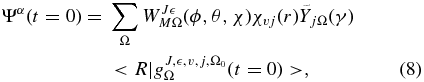
where WJMΩ(ϕ, θ, χ) is a parity-adapted basis set that depends on the ϕ, θ, χ Euler angles, where χvj(r) are the rovibrational eigenfunctions of the H+2(v, j) product,  are normalized associated Legendre polynomials, and
  is a real superposition of the incoming and outgoing Gaussian functions. The radial variables r and R are described in finite grids of equidistant points, while γ is represented by Gauss–Legendre quadrature points. Ω is the helicity quantum number, i.e., the projection of the total angular momentum on the body-fixed z-axis. For the reactive system considered in this work, it has been demonstrated that it is more convenient to use product Jacobi coordinates (r', R', γ') given the mass combinations (Gómez-Carrasco & Roncero 2006). In particular, if product Jacobi coordinates are employed, the number of angular grid points necessary to obtain converged results is reduced from 220 to 192. When using product Jacobi coordinates, the initial wave packet (WP) is transformed from reactant to product coordinates. As a result, the initial WP expressed in product Jacobi coordinates is a superposition of different Ω' values (Zanchet et al. 2010).
The relevant parameters used in the TDWP–CC calculations were chosen so that the total J = 0 probabilities as a function of collision energy were well converged and are listed in Table 1. The calculation of the reaction probabilities for J > 0 would require the inclusion of all possible helicity Ω' projections. Because including all Ω' projections for high J values would be very demanding, the helicity basis used was truncated, so that Ω' ⩽ |Ω'| ⩽ min (J, Ω'max ), with Ω'max = 7 in this case. The convergence of the reaction probabilities with Ω'max will be discussed in the next section. The TDWP–CC calculations were carried out in the collision energy range 0.005–1.0 eV and for the LiH reagent rovibrational quantum state (v = 0, j = 0). A test calculation of the reaction probability as a function of the collision energy was carried out for J = 0 to check for convergence using the time-independent QM methodology as implemented in the ABC code (Skouteris et al. 2000) in the same collision energy range. In this case, the following parameters have been used: the maximum rotational quantum number is 41, the maximum internal energy in any channel is 1.8 eV, the maximum hyperradius is 40.0 Bohr, the number of log-derivative propagation sectors is 500, and the collision energy increment is 0.001 eV.
Table 1. Parameters Used in the TDWP–CC Calculations (All Distances are Given in Å)
| Product scattering coordinate range | Rmin = 0.7; Rmax = 26.0 |
| Number of grid points in R | 320 |
| Diatomic coordinate range | rmin = 0.3; rmax = 26.0 |
| Number of grid points in r | 256 |
| Number of angular basis functions | 192 |
| Center of initial wave packet | R0 = 22.0 |
| Initial translational kinetic energy/eV | Ecoll = 0.372 |
| Position of the analysis line | R∞ = 21.0 |
| Number of Chebyshev iterations | 80000 |
Download table as: ASCIITypeset image
The calculation of the ICS as a function of the collision energy for an initial rovibrational state v, j of the reagent molecule, σR(Ecoll; v, j), requires summing up all the partial wave contributions of the total angular momentum J to the reaction probabilities (Alagia et al. 2000; Aoiz et al. 2005):
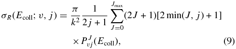
where k2 = 2μrEcoll/ℏ2 and PJv, j(Ecoll) is the reaction probability from the initial rovibrational state v, j summed over all the final states as a function of the collision energy, Ecoll, at a total angular momentum J, which can be written in terms of the S matrix elements as

To reduce the computational effort, the TDWP–CC calculations are performed only for selected Ji total angular momentum values, from J = 10 to J = 110 in steps of 10. The reaction probabilities for intermediate Ji < J < Ji + 1 values are obtained using a linear interpolation (Defazio & Petrongolo 2009) using the reaction probabilities obtained by extrapolation of  and
and  via the J-shifting technique (Bowman 1985), as
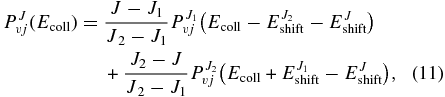
where  is the energy threshold for Ji (i = 1,2) and EJshift is obtained using a quadratic expression in J:

where the A, B, and C constants are evaluated by fitting the energy thresholds of the reaction probabilities obtained for the selected Ji values. The reliability of this interpolation procedure will be examined in the next section.
The v, j initial state-selected rate constants are calculated by averaging the corresponding ICS, σvj(Ecoll), over the translational energy as
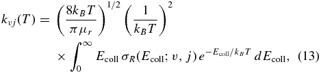
where kB is the Boltzmann constant and μr is the reduced mass of the reactive system.
3. RESULTS AND DISCUSSION
Figure 1 depicts the total reaction probability as a function of the collision energy, PJ = 0(Ecoll), for the H++LiH(v = 0, j = 0) → Li+H+2 reaction calculated at J = 0 using the TDWP–CC methodology. As can be seen, PJ = 0(Ecoll) shows no threshold, reaching an average value of ≈0.9 at the lowest collision energies. The most salient feature of PJ = 0(Ecoll) is its extremely congested resonance structure manifested as sharp oscillations whose amplitude progressively decreases with increasing collision energy. This resonance structure may be expected from the existence of deep wells in the reactant and product valleys that support many metastable states above the dissociation limit of the LiH+2 molecular ion. As the collision energy increases, the resonances become broader and less pronounced, reflecting the shortening of the lifetime of the collision complexes. Apart from the oscillations, the average reaction probability displays several maxima (≈0.1 and 0.3 eV, and a much shallower one at 0.7 eV). At the highest energies calculated here, its value decreases to 0.1.

Figure 1. Total reaction probability as a function of collision energy calculated at J = 0 for the H++LiH(v = 0, j = 0) → Li+ H+2 abstraction channel. Black solid line: TDWP–CC calculations. Red dashed line: TIQM calculations. Previous calculations from Bulut et al. (2008), Pino et al. (2008), and Bovino et al. (2010) are also depicted as indicated in the legend.
Download figure:
Standard image High-resolution imageThe reaction probabilities calculated using different methods are also compared in the figure. In particular, there is a consistently good agreement between the TDWP results and those calculated using the time-independent quantum mechanical (TIQM) method implemented in the ABC code (Skouteris et al. 2000). Some discrepancies are, however, observable in the fine structure due to the numerous resonances whose precise location and magnitude may differ depending on the method and the detail of the calculations. In any case, it is important to remark that the TDWP and TIQM calculations predict the same behavior in the whole range of collision energies and most especially at Ecoll < 0.2 eV. This is quite reassuring because it is known that, in general, it is difficult to get well-converged TDWP results at low energies due to the need for long propagation times and well-adjusted absorbing functions at the edges of the grid. The corresponding results of the QCT (Bulut et al. 2008; Pino et al. 2008) and QM–NIP calculations (Bovino et al. 2010) are also shown in Figure 1 for comparison. They approximately reproduce the overall shape of the present TDWP and TIQM PJ = 0(Ecoll), although with some noticeable discrepancies, depending on the method used. The discrepancies found between the present TDWP and TIQM calculations and the QM–NIP results are especially remarkable. The QM–NIP calculations do not reproduce the broad maximum obtained at the 0.1–0.15 eV collision energies and clearly underestimate the reaction probabilities at collision energies above 0.6 eV. As can be expected, the QCT reaction probability is just a coarse picture of the QM results, but approximately reproduce the location and heights of the various maxima.
As we have mentioned in Section 2, the calculations of total reaction probabilities for J > 0 have been performed using a maximum value of the helicity of Ω'max = 7. In Figure 2, the reaction probabilities for J = 30, PJ = 30(Ecoll), using Ω'max = 0, 3, 5, and 7 for the H++LiH(v = 0, j = 0) → Li+H+2 reaction are compared to each other. As can be seen, it is necessary to include up to Ω'max = 7 to converge the total reaction probability in the considered energy range. Similar results and conclusions have been obtained for J = 50 (not shown).

Figure 2. Total reaction probability as a function of collision energy for J = 30 and Ω'max = 0, 3, 5, and 7 for the H++LiH(v = 0, j = 0) reaction.
Download figure:
Standard image High-resolution imageIt must be noted that the calculation with Ω'max = 0 is equivalent to a CS approximation calculation and it is clear that the reaction probability is much smaller than the calculation corresponding to Ω'max = 7. This is conclusive proof that the CS approximation will fail to account for the reaction probabilities at the necessary J values in order to determine cross sections and rate coefficients. As reviewed by Chu & Han (2008), the CS approximation usually fails in describing ion–molecule or atom–molecular ion collisions, either with a barrier or a deep well.
As explained in Section 2, the reaction probabilities for intermediate Ji < J < Ji + 1 values not evaluated by the TDWP–CC method are obtained using a combination of a linear interpolation and a J-shifting technique. In order to illustrate the accuracy of this procedure, the reaction probabilities for J = 10 and J = 30 computed using the TDWP–CC method and the interpolation method are compared in Figure 3. As can be seen, the agreement is very satisfactory and lends credence to the use of interpolation methodology to determine intermediate J reaction probabilities.

Figure 3. Total reaction probability as a function of collision energy for J = 10 (top) and J = 30 (bottom). Black solid line: TDWP–CC. Red dashed line: interpolation.
Download figure:
Standard image High-resolution imageFigure 4 depicts a log–log plot of the excitation function, σR(Ecoll), for the title reaction obtained using the TDWP–CC calculations according to the methodology presented in Section 2. In the collision energy range from 0.005 up to 1 eV, the cross sections were obtained from the TDWP–CC reaction probabilities calculated at selected values of the total angular momentum J between 0 and 110, using, as described in Section 2, the J-shifting interpolation procedure for those J values where computations were not performed. For collision energies below 0.005 eV (which are needed to evaluate the rate constants at very low temperatures), the excitation function has been extrapolated considering a Langevin model of the type σR(Ecoll) = AE−1/2coll. The parameter A = 8.0 ± 0.5 Å2 ·(eV)1/2 has been obtained by fitting the TDWP–CC cross sections in the energy interval 0.005–0.01 eV to such a functional form. The reason for this extrapolation lies in the great difficulty in converging the TDWP results at Ecoll below 0.005 eV and, hence, in accurately determining reaction, probabilities at very low collision energies. On the other hand, it is expected that the excitation function will follow the Langevin model at very low energies.

Figure 4. Total reaction cross section as a function of collision energy for the H++LiH(v = 0, j = 0) → Li+ H+2 reaction. Black solid line: TDWP–CC. Blue thin solid line: TDWP–capture model. Green dash-dot-dot line: QCT. Red dashed line with circles: QM–NIP. Orange dash-dotted line: Langevin model σR(Ecoll) = AE−1/2coll with A = 8.0 ± 0.5 Å2 ·(eV)1/2. The TDWP-capture model and QCT results are taken from Bulut et al. (2008). The QM–NIP results are taken from Bovino et al. (2010).
Download figure:
Standard image High-resolution imageThe corresponding excitation functions for the same reaction, obtained in the previous TDWP-capture model and QCT calculations by Bulut et al. (2008) and the QM–NIP calculations (Bovino et al. 2010) on the same PES, are depicted in Figure 4. As can be seen, a reasonable agreement is observed between the present accurate TDWP–CC total ICS and those obtained using the previous TDWP-capture model and QCT calculations. In contrast, the QM–NIP cross sections (Bovino et al. 2010) are well above the present results for collision energies above 0.005 eV (sometimes by a factor of 10), but then they fall below the Langevin model for energies below 0.001 eV (note that the comparison is carried out in a log–log plot). It is interesting to point out that the TDWP–CC, TDWP-capture model, and QCT excitation functions show values of the cross section smaller than 15 Å2 at collision energies above 0.1 eV, but below that energy, the cross section rapidly increases to values in the range of 100–150 Å2, as expected for an ion–molecule reaction with no barrier. It must be noted that the large disagreement found between the present excitation function and that calculated by Bovino et al. cannot be justified by the differences observed in the reaction probabilities at J = 0 (see Figure 1). Thus, the origin of the disagreement has to be found in the reaction probabilities for J > 0, obtained by the CS approximation in the work of Bovino et al.
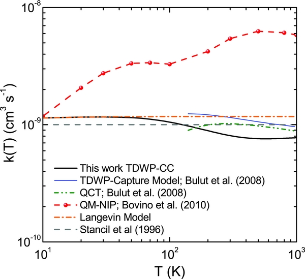
The excitation function calculated using the TDWP–CC method has been used to evaluate the specific rate coefficient for the title H++LiH(v = 0, j = 0) → Li+H+2 reaction in the temperature range of 10–1000 K. The rate coefficients obtained in this work are compared in Figure 5 with the previous calculations using the TDWP-capture model and the QCT method (Bulut et al. 2008), the QM–NIP method (Bovino et al. 2010), and the estimated rate coefficients by Stancil et al. (1996). As can be seen, the present TDWP–CC rate coefficients are nearly independent of temperature and are in quite good agreement with the predicted rate coefficients of the TDWP-capture model and the estimated values by Stancil et al. In contrast, the calculations with the QM–NIP method yield rate coefficients that decrease with decreasing temperature and are almost one order of magnitude larger than the TDWP–CC rate coefficients at high temperatures.
Figure 5. Rate coefficients for the H++LiH(v = 0, j = 0) → Li + H+2 reaction. Black solid line: TDWP–CC. Blue thin solid line: TDWP-capture model. Green dash-dot-dot line: QCT. Red dashed line with circles: QM–NIP. Orange dashed line: rate coefficients from a Langevin model. The TDWP-capture model and QCT results are taken from Bulut et al. (2008). The QM–NIP results are taken from Bovino et al. (2010). The estimated value of 10−9 cm3 s−1 by Stancil et al. (1996) is shown as a horizontal grey line.
Download figure:
Standard image High-resolution image
4. CONCLUSIONS
In this work, we have applied an accurate TDWP–CC method to study the reactivity of the H+ + LiH → Li + H+2 reaction on the ab initio PES developed by Martinazzo et al. Using this method, which treats the Coriolis coupling rigorously, it has been shown that it is possible to obtain converged total reaction probabilities with respect to the helicity Ω' projections with Ω'max = 7, and that the CS decoupling approximation fails to predict their accurate values. The reaction probabilities have been computed for selected values of the total angular momentum, J = 0, 10, 20, 30, 40, 50, 60, 70, 80, 90, 100, 110, and a variant of the J-shifting interpolation method has been employed to determine the excitation function for collision energies from 0.005 to 1 eV. Good agreement is found with the corresponding excitation function and rate coefficients for the same reaction obtained in the previous TDWP-capture model and QCT calculations by Bulut et al. (2008). All the corresponding excitation functions follow approximately the E−1/2coll law, as expected for a barrierless exothermic reaction and, hence, predict rate coefficients essentially independent of temperature. In contrast, the QM–NIP excitation function obtained by Bovino et al. (2010) for the same collision energy interval deviates from this trend. The discrepancy may be due to the fact that the CS approximation fails to capture the correct dynamics of the system. The present rate coefficients are found to be in good agreement with the estimates employed in the evolutionary models of the early universe lithium chemistry.
N.B. acknowledges a grant by Universidad Complutense de Madrid under the program "Programa de doctores y tecnólogos en la UCM-Grupo Santander." Financial support from the Scientific and Technological Research Council of Turkey (TUBITAK) (Project No. TBAG-109T447) and Firat University Scientific Research Projects Unit (FUBAP-1775) is gratefully acknowledged. TDWP computations have been performed on the High Performance and Grid Computing Center (TR-Grid) at ULAKBIM/Turkey. The authors also acknowledge funding from the Spanish Ministry of Science and Innovation (grants CTQ2008-02578/BQU and Consolider Ingenio 2010 CSD2009–00038). This research was conducted within the Unidad Asociada Química Física Molecular between UCM and the CSIC.