


ABSTRACT
In order to distinguish the leptonic from the hadronic origin of the non-thermal emission of a flaring blazar, we present a semi-analytical model that describes the temporal development of the emergent particles (i.e., photons and neutrinos) based on their leptonic and hadronic origins, respectively. The approach starts with the transport equation of the injected relativistic particles and takes spatial diffusion and continuous energy losses into account. On the one hand, a relativistic electron pick-up is considered, which leads to synchrotron, as well as external Compton emission; and on the other hand, a relativistic proton pick-up, which results in high-energy photons and neutrinos by inelastic proton–proton collisions. The temporal development of the emergent photon and neutrino intensities of blazar flares in hadronic and leptonic interaction scenarios are calculated, given useful predictions of flare durations and time lags between photons of different wavelength and high-energy neutrinos.
Export citation and abstract BibTeX RIS
1. INTRODUCTION
The primary hadronic or leptonic nature of the non-thermal radiation production in active galactic nuclei (AGNs) is still an unsolved problem in high-energy astroparticle physics and the detection of extragalactic high-energy neutrinos could become the smoking gun evidence. One of the most promising AGNs with reference to the open questions of AGN physics belongs to the blazar class, which is characterized by high luminosity, short time variability, and high polarization of the observed radiation. Currently, several multifrequency campaigns on flaring blazars have shown a strong correlation between optical, X-ray, and TeV emission (Aharonian et al. 2009; Donnarumma et al. 2009; Vercellone et al. 2010), which indicates the same origin of this non-thermal radiation. There are four effects determining the temporal behavior of the emission volume: (1) the initial condition of relativistic particles, its subsequent (2) spatial diffusion and (3) continuous cooling processes, as well as (4) propagation effects of the generated particles (i.e., photons and neutrinos, respectively) in the emission knot.
Recently, Eichmann et al. (2012, hereafter referred to as ESR12) have considered the effects (1)–(4) and developed a model to calculate the time-dependent synchrotron radiation of a blazar by using different injection scenarios. Here, we extend the study, as we account for the excitation of electrostatic turbulences by the relativistic particle beam, as well as the effects of energetic dependent spatial diffusion. Furthermore, we calculate the external Compton (EC) radiation by using the δ-function approximation (Dermer & Schlickeiser 1993) for inverse Compton scattering of relativistic electrons and evaluate the emission of gamma-rays and neutrinos by inelastic p–p interactions in a hadronic emission model, taking the energy spectra of the secondary particles by Kelner et al. 2006. Hence, the calculations offer a systematic study of the temporal behavior of flaring blazars based on the leptonic and hadronic nature of the primary particles, respectively. As the intergalactic medium consists mostly of ionized hydrogen, the relativistic pick-up particles are very likely electrons and protons. The particle density of the plasmoid is much higher than the density of the ambient medium and thus the plasmoid conditions, i.e., the magnetic field and the background plasma, determine the distribution of the injected particles and the transport equations of the relativistic electrons and protons are not entangled. We consider a spherical emission knot of radius R = 1015R15 cm that is Doppler boosted toward the observer and consists of a non-relativistic plasma of electrons and protons of density Nb = 1010N10 cm−3. Using such a high particle density in the emission volume, we obtain significant pion production by p–p interactions (Pohl & Schlickeiser 2000) and a diffusive buildup of synchrotron photons in the interior, as the optical depth τ = σTNbR > 1. Furthermore, the resulting neutrino flux at 1 TeV is shown to be above the current detection limit of IceCube, which is the most sensitive high-energy neutrino observatory to date.
Since injection durations smaller than the light travel time in the emission knot are negligible (ESR12), we apply an instantaneous pick-up at the time t = t0 with a low particle density q0 = 10−4 q−4 cm−3 and an initial Lorentz factor γ0 = 106γ6. Consequently, the radiation processes by synchrotron self-Compton (SSC) are negligible, as q0 < 109 R−115 γ−20 (Schlickeiser et al. 2010) and in Appendix A.1 we show that also the photohadronic interactions are insignificant at Lorentz factors γ6 < 7.3 θ−11, where θ = 10θ1 eV refers to the energy of the thermal photon field. However, there are still parameters (like the magnetic field strength, the external photon density or the radius of the emission knot) which are in general not confined by our model. Since the parameters of AGN jets are rather unknown and it is not the aim of this paper to verify them, the used limits refer only to dominant EC and proton–proton pion emission.
This paper is structured as follows: first we solve the transport equation of relativistic electrons and protons in the emission volume. Second, we calculate the emergent intensity of photons and neutrinos, respectively, considering only the primary relativistic electrons (Section 4) and protons (Section 5). Finally, we compare the temporal emission behavior resulting from the leptonic and hadronic ansatz and give some useful predictions of the time of maximal flare emission and the flare duration.
2. RELATIVISTIC ELECTRONS AND PROTONS
All physical quantities are calculated in a coordinate system comoving with the radiation source.
2.1. Kinetic Equation of Charged Particles
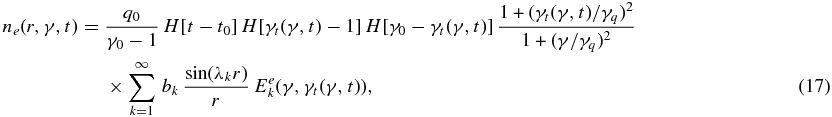
The differential number density of relativistic electrons ne(r, γ, t) and protons np(r, γ, t), respectively, obey the transport equation of ESR12 and takes spatial diffusion, continuous energy losses, and a separable injection term q1(γ, t)q2(r) into account:

Here we idealized that the spatial diffusion is independent of its solid angle, as the anisotropy becomes negligible with increasing time and decreasing Lorentz factor, respectively. Furthermore, the captured relativistic electrons and protons may increase their energy in the emission knot by distributed stochastic acceleration (Schlickeiser & Dermer 2000) and diffusive shock wave acceleration processes (Ball & Kirk 1992; Kirk et al. 1998). However, we do not consider these processes here: (1) stochastic gyroresonant acceleration from dust induced turbulence (Schlickeiser & Dermer 2000) depends sensitively on the details of providing low-frequency MHD turbulence with multiple phase speeds, (2) a relativistic shock (driven by the emission knot) may form upstream of the emission knot by escaping charged particles from the knot (Gerbig & Schlickeiser 2011), but its collision-free properties will be different from pure hydrodynamical shocks.
Our energization of relativistic particles in the emission knot only relies on the relativistic pick-up process (Pohl & Schlickeiser 2000) with subsequent plateauing (Pohl et al. 2002).
According to ESR12 the initial spatial distribution of the injected particles has no significant influence on the temporal synchrotron flare behavior, so that we initially assume them to be homogeneously distributed in the whole emission volume, i.e., q2(r) = 1. The injected particle beam excites electrostatic turbulences, whereby the particles' energy is quickly changed until a plateau distribution in p∥ is established (Pohl et al. 2002), so that the injected particles can be considered as plateau distributed and we obtain

Additionally, electromagnetic turbulences (i.e., Alfvén waves) are excited, which result in pitch angle scattering of the injected charged particles with an energy dependent diffusion coefficient D1(γ). We assume an isospectral power-law turbulence with a spectral index 1 ⩽ q ⩽ 3, so that the spatial diffusion coefficient is determined by (Schlickeiser 2002)

with the magnetic turbulence ∂B, the minimum wavenumber kmin, and the Larmor radius 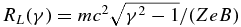 of the relativistic particle. The function F is only determined by the charge Z of the particle, as well as the spectral index q and the helicity parameters which are all independent of the energetic properties of the particle. In the same way, the minimum wavenumber kmin only refers to the maximum Alfvén wavelength λmax = 2πk−1min, which has to be smaller than the size R of the emission knot. In general, the diffusion coefficient is also a function of r and t, as the magnetic field adjusts itself to the actual energy density of the radiating particles (Schlickeiser & Lerche 2008). But we ignore this nonlinear behavior in order to solve the differential equation (1). However, in the special case of q = 2 Equation (3) becomes independent of the Larmor radius and the diffusion coefficient is a constant, as we expect a similar spatial and temporal dependency of the magnetic field B and its perturbation δB. Since most of the microphysical details of the turbulence are unknown, we summarize some of the parameters of Equation (3) by the energy independent mean free path le, p of the electron and proton, respectively. Thus, in the full diffusion limit le, pγβ0 ≪ R the spatial diffusion coefficient at relativistic particle energies (γ ≫ 1) yields

where β = 2 − q.
Furthermore, the relativistic particles cool by different continuous energy loss effects. In case of the relativistic electrons ESR12 have shown that the energy loss is caused by synchrotron and EC effects at high energies and Coulomb interactions with the background plasma at small energies, so that

Here we assume a magnetic field of constant strength B = 1 b G, which is randomly distributed on scales larger than the Larmor radii of the injected electrons, as well as a constant density Nb = 1010N10 cm−3 of the fully ionized background plasma. Furthermore, lEC = 0.093 L46 δ21 τ−2 R−2pc refers to the EC losses due to an isotropic external photon field (Dermer & Schlickeiser 1994), which depends on the luminosity Lad = 1046 L46 erg s−1 of the accretion disk, the scattering optical depth τsc = 10−2 τ−2 and the extension Rsc = 1 Rpc pc of the scattering gas, as well as the Doppler factor δ = 10 δ1 of the emission volume.
In the case of relativistic protons the cross section of electromagnetic interactions is much smaller than that of electrons with the same Lorentz factor, as the Thomson cross section for a proton σT, p = 3 × 10⁻⁷ σT, e, where σT, e is the Thomson cross section for an electron. Thus, the relevant interaction processes are on the one hand hadron–photon interactions with the accretion disk photons with a thermal energy θ = 10θ1 eV and on the other hand hadron–hadron interactions with the thermal background plasma. However, at a particle density N10 > 2.7 × 10⁻⁸ δ21 L46τ−2 R−2pc θ−11 and a Lorentz factor γ6 < 7.3 K θ−11, the dominant proton energy loss rate

results from inelastic interactions with the protons of the background plasma (see Appendix A.1).
2.2. Solution of the Particle Kinetic Equation
In spite of the energy dependent diffusion coefficient D1(γ), the radial diffusion operator is still a Sturm–Liouville type and thus we solve the kinetic transport Equation (1) according to ESR12 in the eigenspace of the operator by using the spatial boundary conditions:
- 1.a finite density at the center of the knot; and
- 2.an exclusively outward directed particle flux at the boundary surface of the knot:


Hence, the particle density yields

where in the full diffusion limit le, p γβ ≪ R of many relativistic particle scattering in the knot the eigenvalues are

with kmax ≪ R/(le, p γβ). Using the ansatz

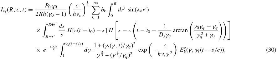
the particle transport Equation (1) becomes

We solve the differential Equation (11) using the Green's function of ESR12, so that the expansion coefficients are

where

and the general functions

as well as

specify the temporal development of the relativistic particle density depending on the particle species. In the case of relativistic electrons the cooling is determined by Equation (5) and thus we obtain

with  . By inserting Equation (12), the relativistic electron density (Equation (8)) yields
in which

and
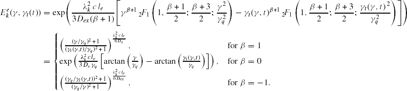
Equation (6) defines the cooling in the case of the relativistic protons and hence with

the relativistic proton density is calculated by

where

and

Figure 1 shows that the continuous energy losses of the relativistic particles result in an increase of the number density (at a Lorentz factor γ < γ0) with increasing time. The electrons cool much faster than the protons by inelastic p–p interactions. In the case of the full diffusion limit (R ≫ γβ0le, p), the different spatial diffusion assumptions (4) have no influence on the particle density, so that the emergent intensity of the generated photons and neutrinos, respectively, is also independent of the spatial diffusion behavior of the relativistic particles. Only the cooling mechanisms determine the temporal development. Thus, the relativistic particles cool down to γ = 1 and due to the third Heaviside function in Equation (17) we obtain for γ0 > γq the maximal electron-generated flare duration

A similar result was already given by ESR12 and hence the energetic distribution of injected particles, as well as the spatial diffusion, has no influence on the upper limit (Equation (24)). In the case of the relativistic protons, the second Heaviside function in Equation (21) yields the maximal proton-generated flare duration

Consequently, an AGN flare generated by relativistic protons can last significantly longer than a flare that is produced by relativistic electrons when the background particle density N10 < 16.7 (b2 + lEC) (1 + ln (γ6)/ln (106))2. However, we have to consider the different particle production rates of each emission process in order to obtain a detailed description of the temporal flare behavior of photons and neutrinos.
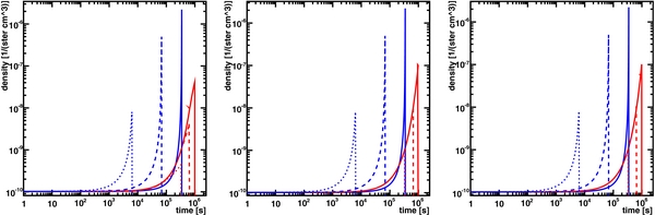
Figure 1. Temporal development of the differential number density of relativistic electrons (blue) and protons (red) at r = 0.1 R in the full diffusion limit, resulting from a spatial homogeneous injection into the whole emission knot. We used a Lorentz factor of γ = 103 (solid line), γ = 104 (dashed line), and γ = 105 (dotted line), as well as β = 1 (left panel), β = 0 (middle panel), β = −1 (right panel), R15 = 1, γ6 = 1, q−4 = 1, and b = 1.
Download figure:
Standard image High-resolution image3. LEPTONIC EMISSION
In this section we consider the radiation resulting from the relativistic electrons of Equation (17) and neglect any further relativistic electrons such as secondary electrons in the emission region.
3.1. Synchrotron Radiation
First, we calculate the synchrotron photon emission generated by the relativistic electron density distribution (Equation (17)). According to ESR12 the spontaneous synchrotron emission coefficient js(r, ν, t) that results from an isotropic relativistic electron distribution ne(r, γ, t) yields

with P0 = 2.647 × 10⁻¹⁰ eV s−1 Hz−1 and the characteristic frequency νs γ2 = 3eBγ2/(4πmec). For an optically thin source, the synchrotron intensity on the surface (r = R) at a time t and an energy  = hν is calculated by (Gould 1979)

with the omnidirectional photon production rate

where the exponential term expresses the survival probability of traveling the distance  from the initial spherical coordinates r', μ' = cos ϕ' to the boundary surface of the knot (Lightman & Zdziarski 1987). Here x = hν/(mec2) is the dimensionless photon energy and
with τKN(x) = R Nb σKN(x)/3, in which σKN(x) denotes the total Klein–Nishina cross section. We use Equation (17) and account for the Heaviside functions in the first integrand, so that the synchrotron intensity (27) yields
where

According to Appendix A.2 the Heaviside functions split the integral expression in several integrands, which are finally solved numerically by a 40-point Gaussian quadrature rule.
Due to the synchrotron cooling of the relativistic electrons the amplitude of the emergent intensity, as well as the total flare duration and the time of maximal synchrotron flare emission, increase with decreasing photon energy (see Figure 2).

Figure 2. Temporal development of the emergent synchrotron intensity at an energy = 1 eV (solid line), = 100 eV (dashed line), and = 1 keV (dotted line). Furthermore, we used β = 0, le = 1010 cm, R15 = 1, γ6 = 1, q−4 = 1, and b2 + lEC = 1.
Download figure:
Standard image High-resolution image3.2. External Compton Radiation
Second, we consider the inverse Compton scattering of low-energy photons by the relativistic electron density distribution (Equation (17)). Since we assume a low number density of injected particles (q0 < 109 R−115 γ−20) to keep the SSC losses negligible, the seed photons for the inverse Compton scattering result from an external photon field. Here, we consider the accretion disk with a temperature θ = 10 θ1 eV and a Planckian distributed spectral luminosity

where the total luminosity Lad = 1046 L46 erg s−1. Assuming that the intergalactic gas scatters the thermal photons to an isotropic distribution, the external photon field in the frame of the emission knot yields (Dermer & Schlickeiser 1993)

with

and has a spectral maximum at

Using the convenient δ-function approximation for inverse Compton scattering (Dermer & Schlickeiser 1993) in the limit γ ≫ 1 ≫ /(mec2) the spontaneous EC emission coefficient results in

Analogous to the previous section the emergent intensity of EC photons at a time t and an energy Eγ is calculated by

with the omnidirectional photon production rate

Inserting the relativistic electron density (Equation (17)) and including the Heaviside functions in the innermost integral, the emergent EC intensity results in
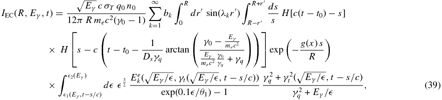
when Eγ > me c2. Here the Heaviside functions yield the integration limits

as well as

Using Appendix A.2 and a 40-point Gaussian quadrature rule, Equation (39) is finally solved analogous to the previous section. Figure 3 shows that the temporal development of the emergent EC intensity is similar to the case of synchrotron radiation and the time of maximal flare emission, and the flare duration increases with decreasing photon energy Eγ. Furthermore, with increasing disk temperature θ the amplitude of the light curves decreases and the time of maximal flare emission shifts to later times, and the flare duration enlarges (especially at low gamma energies Eγ) due to the spectral dependence (Equation (35)) of the maximal external photon density and the δ - approximation in Equation (36).
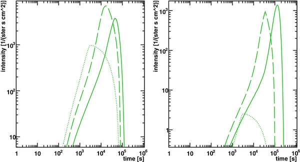
Figure 3. Temporal development of the emergent EC intensity at an energy Eγ = 1 GeV (solid line), Eγ = 10 GeV (dashed line), and Eγ = 100 GeV (dotted line). Furthermore, we used an accretion disk temperature of θ1 = 0.1(left panel) and θ1 = 1, respectively, as well as n0 = 1 cm−3, β = 0, le = 1010 cm, R15 = 1, γ6 = 1, q−4 = 1, and b2 + lEC = 1.
Download figure:
Standard image High-resolution image4. HADRONIC EMISSION
In this section we consider only the relativistic protons of Equation (21) and their interactions with the non-relativistic protons of the background plasma. According to Appendix A.1 the emission knot is considered as a high-density plasma ejection with a small Lorentz factor, so that photohadronic interactions can be neglected. Due to the mathematical complexity, this first approach neglects additional photon products from the secondary electrons (and positrons), which result from the decay of the generated charged pions. However, as the energy spectra of secondary electrons are with approximated good accuracy by the electron neutrinos (Kelner et al. 2006), the temporal behavior of the electron neutrino intensity also shows when the influence of secondary electrons kicks in.
4.1. Gamma and Neutrino Emission by Inelastic p–p Interactions
The relativistic protons with an energy Ep = γ mpc2 collide inelastically with the non-relativistic protons of the background plasma of constant density Nb and generate, among other things, neutral and charged ultrarelativistic π-mesons that decay quasi-instantaneously into gamma-rays (l = γ) and neutrinos (l = {νe, νμ}), respectively, with an energy El. The energy losses of the intermediate particles are also negligible, according to the high mass (in reference to the electron mass) and the short mean lifetime of the pions and muons. In the case of the longer-living muons the mean lifetime in the rest frame of the plasmoid yields τμ ≃ 2.2γμ μs and the energy losses at high Lorentz factors are dominated by synchrotron cooling with the rate  . Thus, the mean total muon energy loss Γμ can be approximated in the first order by

so that the approach Γμ/γμ ≃ 0 is even accurate at the highest considered Lorentz factors when b ≪ 100.
Using the energy spectra F(El/Ep, Ep) of secondary particles in the energy range El ⩾ 100 GeV (Kelner et al. 2006), as well as the cross section of hadronic pion production

the omnidirectional production rate of the particle species l is calculated by

where high-energy photons (x ⩾ 1) and neutrinos have the same escape probability exp (− s/R).
Consequently, the emergent intensity of gamma-rays and neutrinos by inelastic p–p collisions yields
with the upper limit of integration

According to Appendix A.2 we finally compute the emergent intensity (Equation (45)) like in the previous sections.
Due to the slower cooling mechanism (Equation (6)) of the relativistic protons, the flare duration of gammas and neutrinos considerably increases with a decreasing number density Nb of background protons. Furthermore, the flare duration slightly increase with decreasing El, which refers to the energy spectra of the secondary particles, whose maximum is around El/Ep ≃ 0.05–0.1, so that the cooling time of relativistic protons increases with decreasing secondary particle energy in order to obtain this quotient for most of the primary particles. However, the time of maximal emission hardly increases with decreasing El (see Figure 4). Except for the amplitudes of the emergent intensities there is only a marginal difference in the emission of gammas and neutrinos.
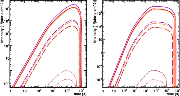
Figure 4. Temporal development of the emergent intensity of gammas (red), muon–neutrinos (magenta), and electron–neutrinos (orange) by inelastic p–p interactions with a background particle density of N10 = 10 (left panel) and N10 = 0.1 (right panel), respectively. We considered the emission at an energy El = 0.1 TeV (solid line), El = 1 TeV (dashed line), and El = 100 TeV (dotted line) and used β = 0, lp = 1010 cm, R15 = 1, γ6 = 1, and q−4 = 1.
Download figure:
Standard image High-resolution imageIn order to observe the calculated neutrino flare with the half-completed IceCube 40 detector the muon neutrino flux has to be above  , where the factor
  has a 90% confidence level and depends on the declination of the neutrino source (Abbasi et al. 2011). Assuming a Doppler factor of δ = 10 δ1, as well as the distance source-observer of D = 1 DMpc Mpc, the intensity of neutrinos with an energy E*ν = δ Eν in the observers frame yields I*ν(E*ν) = 1.1 × 10⁻¹⁶ δ31 R215 D−2Mpc Iν(Eν = E*ν/δ) at the detector. A crude comparison with the detection limit demonstrates that the maximal muon neutrino intensity
  has to satisfy the following relation:

Using Figure 4 we reason that N10 = 1 is the minimal background proton density in order to obtain a detectable neutrino flare with the energy  of a source at 1 Mpc distance and optimal declination condition (
 ). Furthermore, the emergent neutrino intensity also increases by increasing the injected proton density q0, according to Equation (45) and the upper flux limit of the recently completed IceCube 86 detector is expected to decrease slightly (Argüelles et al. 2010).
5. TIME LAGS AND CONCLUSIONS
In the following we summarize the temporal development of the leptonic and hadronic flares and focus on the differences in the time of maximal emission, as well as the half-life of the flare, i.e., the time at which the emergent intensity is decreased to the half of its maximum. The amplitude of the emergent intensity by the leptonic and hadronic scenarios strongly depends on several unknown parameters, like the spatial distribution of seed electrons and protons, respectively, as well as the properties of the emission volume (R, Nb, B) or the external photon field (n0, θ). However, the temporal development of the emergent intensity is mainly defined by the parameters B, θ, and Nb of the particular cooling and emission process. The different spatial diffusion assumptions do not change the flare emission in the full diffusion limit (R ≫ γβ0 le, p). Furthermore, the calculations of ESR12 have shown that the temporal flare behavior is also not affected by the injection assumptions (like the initial energy spectrum), but a finite injection duration Tid ≫ R/c enlarges the flare duration significantly by Tid. Nevertheless, the remaining question is the influence of significant particle acceleration within the emission region and during the flare development.
Based on the leptonic and hadronic scenarios, respectively, Figure 5 shows the half-life of the emergent intensity and the time of maximal flare emission at an energy range from 1 eV up to 100 TeV. The flare duration as well as the time of maximal emission for each radiation scenario increases with decreasing photon energy and/or decreasing cooling parameters B and Nb, respectively. Especially, the EC emission gets increasingly delayed (especially at low Eγ) with decreasing plasma density Nb, whereas the high-energy synchrotron emission is independent of Nb. Furthermore, there is a distinct difference between the hadronic and the leptonic scenario, since the time of maximal emission of gammas and neutrinos by pion production hardly differs by changing the cooling parameter Nb or the energy El. The minimal flare duration is limited by the radius of the emission knot due to the light crossing time R/c and the maximal flare duration is limited by the cooling mechanism of the primary particles according to Equations (24) and (25), respectively. Thus, the relativistic protons can generate significantly longer flare durations than the relativistic electrons, when the background particle density N10 < 16.7 (b2 + lEC) (1 + ln (γ6)/ln (106))2. Another important feature of Figure 5 is the small time lag in the half-life between the neutrino and the gamma-ray emission by p–p interactions, whereas the time of maximal emission shows no difference between neutrino and gamma-ray emission. The steeper decay of the half-life in the case of neutrinos results from the bigger difference in the maximal value of its energy spectra  and
and  , respectively, at different proton energies (see Figures 7–9 in Kelner et al. 2006).
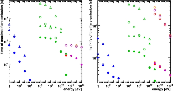
Figure 5. Characteristical temporal features of the emission of synchrotron photons (blue symbols), EC gammas (green symbols), as well as gammas (red symbols), muon-neutrinos (magenta symbols), and electron-neutrinos (orange symbols) by inelastic proton–proton interactions. The features are calculated by using two different plasma densities: N10 = 0.1 (non-filled symbols) and N10 = 10 (filled symbols) and in the case of the leptonic emission scenario we additionally vary the magnetic field strength, so that b2 + lEC ≃ 1 (circles) and b2 + lEC ≃ 0.1 (triangles), respectively. Furthermore, we used θ1 = 1, β = 0, R15 = 1, γ6 = 1, and q−4 = 1 in the full diffusion limit.
Download figure:
Standard image High-resolution imageApart from the intrinsic time lags between photons and neutrinos, we have to discuss other temporal effects on the propagation of these particles. According to Appendix A.3 the high-energy photons are not significantly pair attenuated in collisions with the synchrotron photons of Equation (30). Thus, there is no temporal varying absorption of gamma-rays that results in a further time lag between high-energy photons and neutrinos. However, as shown in Appendix A.4 the finite neutrino mass retards the propagation speed while the neutrinos propagate from the emission knot to the observer, which depends quadratically from the neutrino rest masses and its energy. Since at the current state of knowledge there is a high inaccuracy in the rest masses of the three neutrino flavors (especially in case of muon and tau neutrino) the influence of a finite neutrino mass on the propagation time is indefinite. But using the theoretical upper limit  of the mean rest mass (Fukugita & Yanagida 2003), the retardation of the propagation speed is negligible. In summary, Figure 5 demonstrates that our model yields significant time lags between the time of leptonic and hadronic emission maxima, as well as different flare durations of gammas and neutrinos resulting from a hadronic emission scenario.
This work was supported by the Deutsche Forschungsgemeinschaft through the grants Rh 35/6-1, Schl 201/20-1, Schl 201/23-1 and by the German Ministry for Education and Research (BMBF) through the Verbundforschung Astroteilchenphysik grant 05A11PC1.
APPENDIX
A.1. Continuous Energy Losses of Relativistic Protons
Here we examine the different continuous energy losses of protons with thermal photon and proton fields. Due to the thermal radiation field of the accretion disk with a photon energy θ = 10θ1 eV, the production of K pions by photohadronic interactions occur only for ultrarelativistic protons with a minimum Lorentz factor of (Mannheim & Schlickeiser 1994)

Hence, the photohadronic pion production is negligible for protons with a Lorentz factor γ6 < 7.3 K θ−11. The pair production in the field of the relativistic proton has a smaller minimal Lorentz factor of 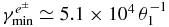 and with the thermal isotropized radiation density of the accretion disk the pair production energy loss rate for protons at threshold yields

The cross section of inelastic proton–proton interactions (Kelner et al. 2006)

can be approximated by the first summand at a Lorentz factor of γ ≪ 1011 and thus we obtain the energy loss rate

of proton–proton pion production. We examine only the case of relativistic protons, so that the Heaviside function equals one. Comparing the rate (Equation (A2)) with (Equation (A4)) yields a dominant energy loss by the hadronic pion production at a density N10 > 2.7 × 10⁻⁸ δ21 L46τ−2 R−2pc θ−11. Furthermore, the Coulomb interactions with the fully ionized background plasma are negligible, as its loss rate

is independent of the parameters much smaller than  .
.
A.2. General Split of a Two-dimensional Integral by Heaviside Functions
In order to calculate the two-dimensional spatial integral expressions of the emergent intensity (30), (39), and (45), respectively, we have to take the limitation of the integrals by the Heaviside functions into account. Hence, we consider the general Heaviside functions H[A − s] and H[s − B], so that after multiple but simple calculations we obtain
After specifying the parameters A and B the emergent intensities can be calculated by a numerical algorithm of integration.
A.3. Photon–Photon Pair Attenuation of Gamma-rays
There are several different matter and photon fields of the inter- or extragalactic medium, which can be discussed in reference to the attenuation of the emitted gamma-rays; however, only a temporal correlated and varying particle field can change the general temporal development (flare duration, time of maximal flare emission) of the high-energy photon intensity (39) or (45). Consequently, the number of relevant interaction particles reduces to those who are related to the initial pick-up of the relativistic electrons and protons, respectively. In the following, we examine the photon–photon pair attenuation with the low-energy synchrotron photons of Section 3.1. From Dermer & Schlickeiser 1994 the absorption coefficient for an isotropic radiation field nph(, r, t) can be approximated by

and the optical depth is determined by

According to ESR12, the emission knot is optically thin for gamma-rays independent of the temporal and spatial development of the synchrotron photon density. Here we confirm this result, when we neglect the spatial, temporal and energetic dependence of the synchrotron photon density Isy(R, = 2m2ec4/Eγ, t)/c and take its maximum Imaxsy/c, so that the maximal optical depth yields

Based on observations of flaring blazars, we consider a maximal luminosity of L* ≃ 1046 erg s−1 at the low synchrotron energies and with a Doppler factor δ = 10 δ1 the emergent synchrotron intensity in the frame of the emission knot becomes Imaxsy(R, = 2me2c4/Eγ, t) ≃ 9 × 10²³ (Eγ/1 TeV) R−215 δ−31 s−1 cm−2. Hence the optical depth yields

and the emission knot is optically thin for gamma-rays independent of its energy. Consequently, there is no relevant systematic influence on the temporal behavior of the emergent gamma-ray intensity.
A.4. Retardation Effects of Heavy Neutrinos
In the following we account for the non-vanishing neutrino mass, which retards the propagation speed and results in a delay between the photon and the neutrino observation. Due to the large distance between the emission knot and the observer, we have to consider the structure of the four-dimensional space-time. In the case of an homogenous and isotropic expansion of the universe, Einstein's field equations yield the Robertson–Walker metric, so that a particle k with the rest mass mk and the energy Ek has at a distance z the delay (Visser 2004)

to a simultaneous produced massless particle. According to the analysis of 307 supernovae type Ia in the redshift range 0.015 ⩽ z ⩽ 1.62 by Guimarães et al. 2009, we assume the Hubble constant H0 = 72 km s−1 Mpc−1, the deceleration parameter q0 = −0.57 and the jerk parameter j0 = −1.
The pion decay generates different neutrino flavors with the mixing ratio νe: νμ: ντ = 1: 2: 0; however, the ratio changes as a result of neutrino oscillation and we obtain νe: νμ: ντ = 1: 1: 1 at a distance much larger than the oscillation length Losc = 4πℏcE Δm−2ij. Consequently, we have to consider the mean neutrino mass  . To date there are only upper limits of the three neutrino masses, so that we can just calculate an upper limit of the delay (Equation (A11)). The experimental observed upper limits (Altarelli & Winter 2003) yield the mean neutrino mass
 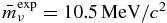 , whereas theoretical considerations claim a maximal neutrino mass of 2.5 eV/c2 independent of the flavor (Fukugita & Yanagida 2003). Figure 6 shows that in the case of the theoretical upper limit the delay is negligible even at large redshifts and small neutrino energies, but in the case of the experimental upper limit the delay (Equation (A11)) can increase to several months or years. Thus, the mean neutrino mass is the crucial parameter and only an improved accuracy of the muon and tau neutrino mass can resolve whether the delay (Equation (A11)) is significant or not. Vice versa, the observation of a delay between a correlated gamma and neutrino flare can be used to determine the mean neutrino mass.
Figure 6. Delay between simultaneous-generated neutrinos and photons dependent of the redshift and the neutrino energy. (a)  ; (b)
; (b)  .
.
Download figure:
Standard image High-resolution image