


ABSTRACT
Based on scanning spectroscopic observations with the Hinode EUV imaging spectrometer, we have found a loop-top hot source, a fast jet nearby, and an inflow structure flowing to the hot source that appeared in the impulsive phase of a long-duration flare at the disk center on 2007 May 19. The hot source observed in Fe xxiii and Fe xxiv emission lines has the electron temperature of 12 MK and density of 1 × 1010 cm−3. It shows excess line broadening, which exceeds the thermal Doppler width by ∼100 km s−1, with a weak redshift of ∼30 km s−1. We have also observed a blueshifted faint jet whose Doppler velocity exceeds 200 km s−1 with an electron temperature of 9 MK. Coronal plasmas with electron temperature of 1.2 MK and density of 2.5 × 109 cm−3 that flow into the loop-top region with a Doppler velocity of 20 km s−1 have been identified in the Fe xii observation. They disappeared near the hot source, possibly by being heated to the hotter faint jet temperature. From the geometrical relationships of these phenomena, we conclude that they provide evidence for magnetic reconnection that occurs near the loop-top region. The estimated reconnection rate is 0.05–0.1, which supports the Petschek-type magnetic reconnection. Further supporting evidence for the presence of the slow-mode and fast-mode MHD shocks in the reconnection geometry is given based on the observed quantities.
Export citation and abstract BibTeX RIS
1. INTRODUCTION
Solar flares are explosive events on the Sun that produce >10 MK plasmas and high-energy particles by heating and particle acceleration processes. Magnetic reconnection is thought to be a key process for producing solar flares and coronal mass ejections (CMEs) after many discoveries from observations by Yohkoh and Solar and Heliospheric Observatory (SOHO). The following observations provide evidence of magnetic reconnection and its resultant phenomena: (1) cusp-shape arcade structures (Nolte et al. 1979; Moore et al. 1980) with a higher temperature than the inner part (Tsuneta et al. 1992; Tsuneta 1996; Hara et al. 2008); (2) plasma ejecta appearing above flare loops, known as plasmoid or loop ejection (Shibata et al. 1995; Ohyama & Shibata 1998; Hara et al. 2008); (3) loop-top hard X-ray (HXR) source (Masuda et al. 1994; Krucker et al. 2008); (4) turbulent motion seen in emission lines from highly ionized ions known as nonthermal velocity (Grineva et al. 1973; Doschek et al. 1980; Culhane et al. 1981; Antonucci et al. 1982; Tanaka 1986; Khan et al. 1995; Harra-Murnion et al. 1997; Mariska & McTiernan 1999); (5) reconnection inflow from apparent motions of coronal plasmas (Yokoyama et al. 2001; Narukage & Shibata 2006; Hara et al. 2008) and from Doppler shift in a spectroscopic observation (Lin et al. 2005; Hara et al. 2006); (6) hot downflow from apparent motions (McKenzie & Hudson 1999; McKenzie 2000; Asai et al. 2004; Sheeley et al. 2004) and from a spectroscopic observation (Innes et al. 2003); and (7) hot outflow as reconnection outflow from a spectroscopic observation (Wang et al. 2007).
Apart from the SUMER results, most of the observations listed above are from imaging systems. Several flare observations by spectrometers, e.g., the Bragg Crystal Spectrometer (BCS) of Yohkoh (Culhane et al. 1991), could not resolve spatial structures. In these cases, the position of spectroscopic signatures in a flare structure cannot be known without other supporting observations. In addition, coronal observations by imaging spectrometers in the visible and extreme-ultraviolet (EUV) ranges require a significant exposure duration at a single slit position to obtain sufficient photons for high-precision spectroscopy. Hence, the probability of detecting specific plasma motions in a flare structure cannot be high in slow spatial scanning observations. However, spectroscopic observations by scanning spectrometers are at present the only way to diagnose flare-associated plasma parameters such as the line-of-sight Doppler velocity, Doppler line broadening, and enhanced line broadening at a specific point. These parameters cannot be investigated by imaging observations. Spectroscopic observations with multiple emission lines can also provide the temperature structures of solar flares from line pair ratios of two different ionization stages and the electron density of reconnection inflow from density-sensitive line pair ratios. A higher-throughput imaging spectrometer can largely improve the situation for detecting phenomena that are associated with magnetic reconnection with a high probability of success.
The EUV Imaging Spectrometer (EIS; Culhane et al. 2007) on board Hinode (Kosugi et al. 2007) has ∼2 arcsec spatial resolution with the highest throughput so far available in two wavelength ranges of 166–212 Å and 246–291 Å. These wavelength ranges contain many emission lines that are formed at 104.6–107.3 K (Young et al. 2007; Brown et al. 2008). The high throughput available with the Hinode EIS allows high cadence raster scanning for flare hunting, and provides flare spectra with sufficient photons for observing low-emission flares that occur during the course of active-region studies. The probability of detecting flare-associated phenomena can be increased substantially with the EIS scanning imaging spectroscopy. In addition, simultaneous observations of multiple emission lines with EIS may reveal how hot flare plasmas are produced in the outer solar atmosphere by detecting such phenomena at the same time. In particular, plasma flows associated with the magnetic reconnection episodes that give rise to solar flares may be more easily detected.
In the present paper, we report a Hinode EIS observation of a solar flare that occurred on 2007 May 19. The instrument was scanning near the loop-top region at the HXR impulsive phase. The location is thought to be the site of magnetic reconnection that plays a key role in producing solar flares. As we report later, we find an isolated hot loop-top source with significantly enhanced line broadening near the HXR peak time, a fast hot outflow from the nearby site, and an inflow structure flowing to the hot source. These are explained in a framework of the standard magnetic reconnection geometry in Shibata et al. (1995) and Tsuneta (1996), which are extensions of the CSHKP model (Carmichael 1964; Sturrock 1966; Hirayama 1974; Kopp & Pneuman 1976). The uniqueness of the present study is that the region around the magnetic reconnection point was spectroscopically observed with the Hinode EIS in detail at the impulsive phase of a long-duration solar flare. It is demonstrated that the bright loop-top source showing enhanced ion motions is located at the downstream side of the fast-mode MHD shock created by the fast reconnection outflow and that the distance between the reconnection point and the flare loop top is short at the start of a solar flare, impulsive phase, as expected. The structure of the slow-mode MHD shock in the reconnection region and the internal structure within the reconnection outflow are discussed based on emission-line spectroscopy.
2. OBSERVATIONS AND THE SPATIAL CONTEXT
The Hinode EIS observed a solar flare on 2007 May 19 in the active region 10956 (AR10956) located near the disk center. EIS was operated in a slit scanning mode with a 1'' wide slit and 1'' step size. The spatial sampling along the slit is 1''. Twenty-one spectral windows in two EUV bands, 166.3–211.9 Å and 245.8–291.4 Å, were obtained with 40 s exposure duration and each window contains multiple emission lines.
Associated with this flare, Veronig et al. (2008) have reported a filament disappearance and a bright two-ribbon structure in Hα observations, a coronal dimming, and a propagating global wave in the EUV imaging observations along with the occurrence of a CME that resulted in an interplanetary magnetic cloud observed by an in-situ measurement on 2007 May 22 (Liu et al. 2008).
Figure 1(a) shows the X-ray flux from the Geostationary Operational Environmental Satellites (GOES) with an X-ray image from the Hinode X-ray telescope (XRT; Golub et al. 2007; Kano et al. 2008). The flare started at 12:46 UT and reached its peak phase at 13:05 UT, when the X-ray peak level for the 1–8 Å channel is B9.5 or 9.5 × 10⁻⁷ W m−2. It occurred at the western part of AR10956 in the box shown in the Fe xii 195.12 Å raster-scan image (Figure 1(b)). The single raster-scan duration of the whole area in Figure 1(b) was 5 hr. The vertical stripes in the scan area of 317'' × 304'' display periods of eclipse due to the Earth and its atmosphere. Figures 1(c) and (d) show a continuum image and an image of the vertical component of photospheric magnetic fields from the spectropolarimeter (SP) of the Hinode Solar Optical Telescope (SOT; Tsuneta et al. 2008; Ichimoto et al. 2008; Suematsu et al. 2008; Shimizu et al. 2008). A group of small sunspots and largely distributed magnetic polarities is seen in the SP map while ∼10 MK hot plasmas were observed in Fe xxiii at 263.76 Å (Figure 1(e)), Fe xxiv at 192.03 Å, and Fe xxiv 255.11 Å (see Figure 13 in Appendix A). Three representative tick marks are shown by vertical bars in Figure 1(e) to clarify the timing of the EIS scanning observations. The brightest source S1 in Fe xxiii at 263.76 Å appeared near the loop-top region of a loop structure seen in Fe xvi at 262.98 Å (Figure 1(f)) at the HXR peak time that is indicated by dotted lines in Figures 1(a), (e), and (f). The loop is indicated by the arrow in Figure 1(f), and is also seen in Fe xvii at 254.87 Å and in Ca xvii at 192.86 Å (see panels in Figure 13). The right-hand (or west) side of the dotted lines in Figures 1(e) and (f) corresponds to the area observed in the pre-flare stage.
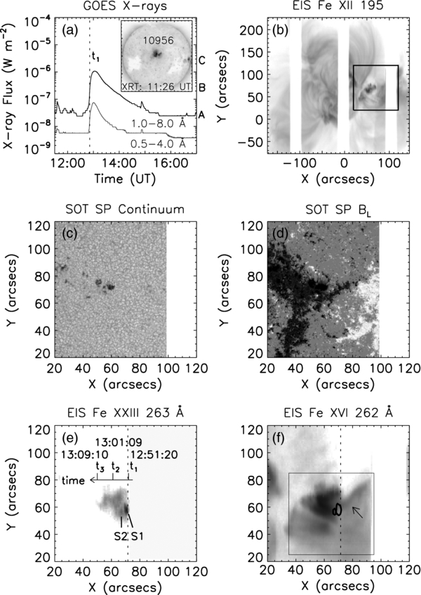
Figure 1. (a) GOES X-ray flux with an X-ray image (Ti-Poly filter) at 11:26 UT. (b) EIS raster-scan map in Fe xii at 195.12 Å with a square showing the area for panels (c) to (f). Vertical white areas show periodic eclipse durations. (c) Continuum intensity and (d) line-of-sight component of magnetic field strength from a SOT SP observation. (e) Hot coronal structures with loop-top sources S1 and S2 in Fe xxiii at 263.76 Å, and (f) in Fe xvii 262.98 Å. Top is north and right is west. Logarithmic and reversed gray scales are used in EUV and X-ray intensity maps. Contours corresponding to S1 and S2 and a square area in panel (f) indicate the bright sources in Fe xxiii and the image area shown in Figures 3, 9, 10, 13, and 19.
Download figure:
Standard image High-resolution imageThe co-alignment among different data sets is performed by using data from the Michelson Doppler Imager (MDI; Scherrer et al. 1995) on SOHO (Domingo et al. 1995) and the Transition Region and Coronal Explorer (TRACE; Handy et al. 1999). The MDI continuum image and magnetogram become a reference for co-alignment to TRACE continuum and SOT SP data. The TRACE EUV coronal images connect EIS and XRT data to be co-aligned to the SP data. The accuracy of the alignment is within 3 arcsec for the whole EIS raster-scan area shown in Figure 1(b). The largest errors originate from the pointing jitter of the scanning spectrometers, because the pointing jitter over the whole scan time was not corrected when the raster-scan data were assembled into a map. The pointing jitter is smaller for a short scanning time corresponding to the small scanning area that is shown in Figures 1(e) and (f). Note that the heliocentric coordinate at 12:47 UT, when the MDI data were obtained, is used for the panels in Figure 1 to allow easy comparison of the different data sets. The coordinate system is fully used throughout this study. Finally, it should be noted that a target region in the EIS long-wavelength band is located to the west of its counterpart in the short-wavelength band by about 2 arcsec (see Appendix B and Figure 14).
The flare was also observed with many imaging instruments, Hinode XRT, TRACE, and the EUV Imager (EUVI) of the Sun–Earth Connection Coronal and Heliospheric Investigation (SECCHI) instruments (Howard et al. 2008) on board the Solar Terrestrial Relations Observatory (STEREO; Kaiser et al. 2008). Figure 2 shows the XRT thick-Be, TRACE 171 Å band and STEREO A EUVI 195 Å band observations with GOES flux light curves. A hot loop is seen in the X-ray image at 12:46 UT, and became bright at 12:52 UT in the flare impulsive phase. Two loop systems are identified; one connects X1 and X2, while the other connects X2 and X3. The footpoints of the loops are rooted on the bright structures observed in the TRACE image at 12:52 UT. It is the so-called bright two-ribbon structure indicated by R1 and R2 in the image with an additional faint ribbon R3. It is known from Figure 1(d) that R1 has positive polarity while R2 and R3 have negative polarity. The bright hot source in Figure 1(e) is located near the loop-top region of the X-ray loop connecting X2 on the ribbon R2 and X3 on the ribbon R1 (see details in Figures 18(a) and (b)). The X-ray loop was cooled down later, and was observed at the arrow in the TRACE 171 Å image at 13:04 UT (Figure 2). The X-ray loop connecting X1 and X2 was also observed at 13:10 UT after cooling down to about 1 MK.

Figure 2. Imaging observations of Hinode XRT (thick-Be filter), TRACE 171 Å, and STEREO A 195 Å with GOES X-ray plot. The hatched area in the GOES plot is the hard X-ray impulsive phase. Logarithmic and reversed gray scales are used.
Download figure:
Standard image High-resolution imageSince there is no counterpart of the Fe xxiii 263 bright source in the TRACE 171 Å image at the impulsive phase (12:52 UT), the hot source S1 must be located in the corona and not near the chromosphere. It may be asked whether the Fe xxiii 263 isolated source S1 could be an artifact due to the change of EUV intensity in a hot loop with time because the EIS was slowly scanning the loop-top region of the X-ray flare loop. However, in Figure 3 we show evidence indicating that the X-ray loop has a faint short-lived loop-top intensity enhancement.
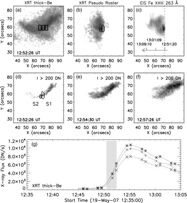
Figure 3. XRT thick-Be filter observations (a) during the hard X-ray impulsive phase, and (d), (e), (f) their contrast enhanced XRT images to find a faint isolated X-ray source near the loop-top region. (b) XRT pseudo raster from a sequence of thick-Be observations simulating (c) EIS Fe xxiii 263 Å raster. (g) Light curves of the XRT observations in square areas shown in panel (a). Plus, asterisk, and cross signs show the X-ray flux in the rectangle box at left, center, and right in panel (a), respectively. Logarithmic and reversed gray scales are used for EUV and X-ray intensity maps.
Download figure:
Standard image High-resolution imageFigure 3(d) is a contrast-enhanced image of Figure 3(a). A faint intensity enhancement is found at S1 denoted by a contour. The area brightened as seen in Figure 3(e), and had faded by the time shown in Figure 3(f). Although these images show that there is a faint local X-ray enhancement in the X-ray loop with a short duration, the pseudo raster-scan X-ray map (Figure 3(b)), which is made from the XRT thick-Be data observed in an interval between 12:46 and 13:12 UT at the EIS slit positions, does not have a clear isolated source, and is rather similar to the EIS Fe xvii raster-scan map in Figure 13. This suggests that the XRT instrument has a better sensitivity for plasmas with a temperature less than 10 MK for the range of multi-temperature flare structure and the differential emission measure of this flare. The X-ray light curves for the three rectangular areas in Figure 3(a) are shown in Figure 3(g). The figure indicates that the intensity of the X-ray loop was increasing at the impulsive phase, and continued up to 12:55 UT, when EIS was scanning the area at the left border of the Figure 3(a) middle box. On the other hand, Fe xxiii 263 intensity drops toward the left border of the S1, while Fe xvi 262 and Fe xvii 254 intensities increase similar to the X-ray flux in the Figure 3(a) middle box. From this information, we speculate that the flare loop has at least two components; one is the hot isolated component near the loop top with a different intensity change with time from the other component that consists of a flare loop structure with a lower temperature.
The above speculation leads to a picture that a hot isolated source is hidden in a bright loop structure with a lower temperature. Figure 4 supports this picture. These three panels (Figures 4(a)–(c)) show the difference images between an image obtained at the flare impulsive phase and the image at the previous timing, in which the solar rotation effect is allowed for. A localized enhancement at the S1 source with a slight extended faint structure to the east–west direction is found in the STEREO A EUVI 195 Å difference image, while it is not in STEREO A EUVI 171 Å and TRACE 171 Å difference images. The EUVI 195 Å band contains the Fe xxiv line at 192.03 Å and the enhancement must be attributed to this line. It provides evidence of an Fe xxiv localized hot source at the flare loop top while the whole flare loop structure like the X-ray loop is not seen in the EUVI 195 Å difference image, suggesting that the Fe xxiv emission of the flare loop is weaker due to a lower temperature.

Figure 4. STEREO A EUV difference images of (a) the 195 Å and (b) 171 Å bands during the flare impulsive phase in reversed gray scale. The enhanced structure in the 195 Å band is found at S1, and is pointed by an arrow. (c) The TRACE EUV difference image at the 171 Å band shows no significant EUV enhancement at the same site.
Download figure:
Standard image High-resolution image3. ANALYSIS
3.1. EIS Spectral Analysis
We used the Solar Software eis_prep routine to correct the dark current and cosmic-ray signals for the EIS raw spectral data. The calibrated spectrum at each data point is fitted by a single Gaussian function to estimate the Doppler velocity and the FWHM. We fit multiple lines by multiple Gaussian components when a spectral window contains multiple emission lines or lines blended with other lines. The tilt of the spectrum on the CCD, a systematic line shift in the spacecraft orbit around the Earth, and the spacecraft Doppler motion with respect to the Sun, are taken into account for estimating the Doppler velocity of purely solar origin.
We select a quiet Sun area outside AR10956, corresponding to the right bottom section in Figure 1(b), at a time prior to the occurrence of the flare as a reference point for the Doppler velocity measurement. The reference wavelengths for the Doppler velocity are the Fe xii (Fe xi) lines at 192.394 Å and 193.509 Å (256.925 Å) for the short- (long-) wavelength band. The reference Doppler velocity of −6 km s−1 (blueshift) in the quiet Sun area is adopted from the measurement of Sandlin et al. (1977). The Fe xii average velocity in the quiet Sun may sometimes be treated as zero velocity in other EIS papers. Fe xi at 256.925 Å is selected as the reference line for the long-wavelength band because it has been regarded as Fe xii until recently identified by Del Zanna (2010). Since the observed Doppler velocity measured in the Fe xii lines at 192.394 Å and 193.509 Å is very close to that in the Fe xi line at 256.925 Å, to within a few km s−1 after the wavelength calibration, the Doppler velocity measurement discussed in the present paper is not affected by the wavelength calibration adopted here.
The instrumental line broadening has been estimated from campaign observations between EIS and a ground-based observatory, Norikura Solar Observatory in Japan, which operated a coronagraph with a high-dispersion scanning spectrometer (λ/Δλ ∼ 1 × 10⁵) and 2'' × 3'' spatial sampling. Appendix C briefly shows how we estimate the instrumental line broadening of the EIS from the campaign data.
3.2. HXR Data Analysis
The HXR data obtained with RHESSI (Lin et al. 2002) are analyzed to understand the characteristics of HXR sources in this flare. For imaging of selected energy bands, we use an image reconstruction method based on the CLEAN algorithm, which is provided in the Solar Software, and is applied to obtain the HXR images. For fine-tuning of photon energy, one of the RHESSI detectors, Detector 1, is used to make the energy spectrum. The analysis of the energy spectrum is also performed using the RHESSI analysis software package in the Solar Software.
4. RESULTS
4.1. A Loop-top EUV Bright Blob at HXR Impulsive Phase
Figures 5(a) and (b) show the relationship between flare structures in the EIS raster-scan observations and HXR sources observed with RHESSI at the impulsive phase, t1, indicated in Figure 5(a), with a corresponding RHESSI HXR photon energy spectrum of two minutes integration time (Figure 5(c)). The HXR spectrum is fitted well in the energy band of 4–30 keV by a combination of a thermal spectrum from a plasma characterized by an electron temperature of 12.0 MK with emission measure of 7 × 1046 cm−3 and a thick-target model that assumes a low-energy cutoff at ∼10 keV in the power-law energy spectrum for high-energy electrons.
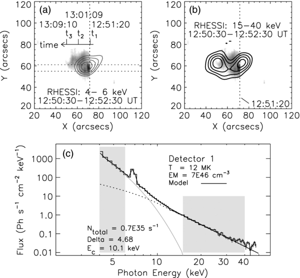
Figure 5. RHESSI synthetic X-ray image contours in (a) 4–6 keV and (b) 15–40 keV energy bands near the impulsive phase (12:50:30–12:52:30 UT) are shown with the EIS raster-scan map in Fe xxiii 263.76 Å. Contour levels are 60%, 70%, 80%, and 90% of each maximum value. Three EIS scanning times (t1, t2, and t3) shown in panel (a) indicate the speed of the raster scan. (c) RHESSI X-ray spectrum near the impulsive phase in solid line. A model spectrum consisting of thermal bremsstrahlung (in gray line), line emission near 7 keV, and a nonthermal component (in dotted line) based on the thick-target model with a low cutoff energy Ec is overlaid in thick line. The energy range of the model fitting is 4–30 keV.
Download figure:
Standard image High-resolution imageThe site of the brightest source in Fe xxiii 263 coincides with the location of the 4–6 keV RHESSI source. There are two high-energy HXR sources at the impulsive phase (Figure 5(b)). One is at the footpoints of flare loops that are located on the bright ribbon structures in the TRACE 171 Å image and the other is found between the two ribbon structures (see Appendix D and Figure 18(a)), suggesting that one of the nonthermal sources appears to be located in the corona close to the hot S1 source. The motion of the centroid of the HXR sources nearly along the X-ray loops is shown in Figures 18(c) and (d). The motion to the west toward the flare peak phase is similar to that is observed in XRT data (Figure 2). It may appear that the co-alignment of the HXR images is inadequate, so that it may be possible to move the RHESSI nonthermal sources by about 10 arcsec for the HXR source on the right to lie on the ribbon structure by sacrificing the positional coincidence between the 4–6 keV HXR source and the hot loop-top source that was observed in EIS, XRT, and STEREO. All the images except for those from RHESSI are co-aligned with the data from full-disk observations with a short difference in the observing time. The remaining positional uncertainty is due to the relation of RHESSI imaging to the solar coordinates. Since we cannot fully check the RHESSI imaging software, and since we do not focus on the high-energy HXR sources in the present paper, we will not argue strongly that the position of the western HXR source is not on the western ribbon structure in TRACE observations. However, the position of the 4–6 keV HXR image at the impulsive phase that coincides with the EIS Fe xxiii bright blob is not just due to coincidence as we will see below.
Figure 6 displays light curves from the RHESSI channels and for the EIS spectral lines for Fe xvii 254, Fe xxiii 263, and Fe xxiv 255 plotted as a function of time along the scanning direction. The spatial averages (EW × NS = 1'' × 7'') along the EIS slit between the two horizontal dotted lines in Figure 5(a) are applied to estimate the parameter values in Figures 6(d)–(h). The Y range for the vertical average is the same as that of each rectangle box in Figure 3(a). The EIS was scanning the area in the Figure 3(a) central box in the interval between 12:50 and 12:55 UT from the right to left. It is difficult to estimate intensities for the Fe xxiii 263 and Fe xxiv 255 lines before the time t1 due to low count rates.
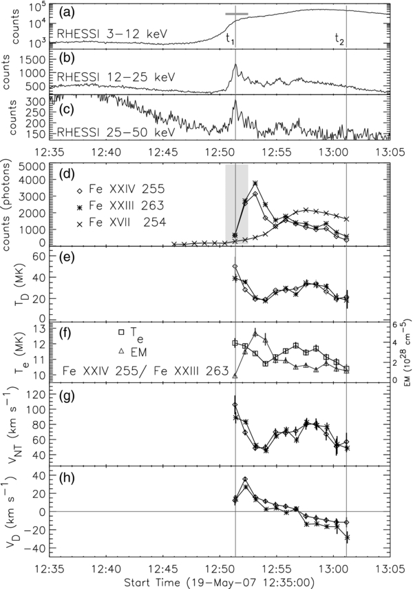
Figure 6. RHESSI X-ray flux in (a) 3–12 keV, (b) 12–25 keV, and (c) 25–50 keV energy bands. EIS observations of (d) EUV flux, (e) Doppler-width temperature TD, (f) electron temperature Te and emission measure EM from line ratio of Fe xxiv 255/Fe xxiii 263, (g) nonthermal velocity VNT, and (h) Doppler velocity VD. Data for Fe xxiii 263, Fe xxiv 255, and Fe xvii 254 are indicated in asterisk, diamond, and cross, respectively. Bright main components, not fast blueshift components, shown in Figures 7(a) and (e) are only presented here. The horizontal bar in panel (a) and hatched area in panel (d) show the integration time to make the RHESSI synthetic maps (Figures 5(a) and (b)) and spectrum (Figure 5(c)).
Download figure:
Standard image High-resolution imageIn the RHESSI light curves, a gradual change in soft X-rays is observed in the 3–12 keV range (Figure 6(a)), while an impulsive HXR structure is seen in higher-energy bands (Figures 6(b) and (c)). The Fe xxiii and Fe xxiv intensities, which are proportional to the number of photons detected and rise and fall sharply in the impulsive phase, correspond to the isolated spatial structure S1 and its eastern part, while the Fe xvii signals show more gradual behavior in the flare loop structure (Figure 6(d)). The soft X-ray light curves in the loop-top region (Figure 3(g)) show a monotonic increase while the EIS was rastering in the region of Figure 3(a) central box. From the comparison with the soft X-ray light curves in Figure 3(g), it is found that the S1 source seen in Fe xxiii and Fe xxiv is an essentially different component from the flare loop observed in soft X-rays, which has been shown as the difference between Figures 3(b) and (c) in the intensity distribution.
Observed Doppler temperatures TD, defined by MiW/(8 ln2 kB), where Mi is the mass of ion, W is the intrinsic line FWHM (with instrumental linewidth removed), and kB is the Boltzmann constant, are high for Fe xxiii and Fe xxiv at the peak of the HXR impulsive phase and then fall rapidly (Figure 6(e)). TD reaches 40–50 MK, implying that the random motion of highly ionized ions is significantly enhanced in the impulsive phase at the loop-top region.
Figure 6(f) shows the electron temperatures deduced from the line intensity ratio of Fe xxiii 263 and Fe xxiv 255 assuming ionization equilibrium. We used the CHIANTI spectral software package (Dere et al. 1997, 2009; Landi et al. 2006) with the ionization fractions of Mazzotta et al. (1998) and the coronal abundances of Feldman (1992) to obtain the line-ratio temperature relations from the contribution function of each emission line. The electron temperature of 12 MK at the impulsive phase is consistent with that of the RHESSI thermal source that is located at the same position in the plane of the sky. The emission measure of the bright blob EMblob is ∼4 × 1028 cm−5.
Nonthermal velocities VNT in Figure 6(g) are derived from the Doppler temperature TD and electron temperature Te. The resulting values show that VNT ∼ 100 km s−1 is observed at the HXR peak time of the impulsive phase, but the value falls rapidly as the Fe xvii signals representing a lower-temperature structure increase. Such nonthermal velocities have been reported by spectrometers with no spatial resolution (Grineva et al. 1973; Doschek et al. 1980; Culhane et al. 1981; Antonucci et al. 1982; Tanaka 1986; Khan et al. 1995; Harra-Murnion et al. 1997; Mariska & McTiernan 1999) and from SUMER observations (Doschek 2006). Our EIS observation, which is indirectly supported by an independent observation at Norikura Solar Observatory for estimating the EIS instrumental width (see Appendix C), identifies an isolated component at 12 MK electron temperature, showing an enhanced ion motion that appears at the loop-top region of the flare loops during the impulsive phase.
Figure 6(h) shows that the component showing enhanced nonthermal velocities or bright Fe xxiii/xxiv intensities near the HXR peak time shows a redshift, while the area of the bright Fe xvii loop top corresponding to scanning points at 12:58–13:01 UT or the area of the left rectangular box in Figure 3(a) shows a blueshift in the Fe xxiii/xxiv observations. This suggests that the former is created by a heating mechanism occurring in the high corona, while the latter could come from the bottom of the corona due to upward chromospheric evaporation flows.
An isolated dense blob moving downward has been found at the loop top in an MHD simulation of a solar flare by Yokoyama & Shibata (2001), which shows the dynamics of the Petschek-type magnetic reconnection. The blob is created by the fast MHD shock at the colliding site of the reconnection jet with flare loops located below and shows a downward motion with a low velocity. The bright blob showing a redshift with a high nonthermal velocity of ∼100 km s−1 in the EIS observation is possibly an example of the dense blob in the MHD simulation by Yokoyama & Shibata (2001). If the bright isolated hot source observed with EIS is actually created by the fast-mode MHD shock, a high-speed jet, a density jump or a density increase at the bright blob, and a temperature jump or a higher temperature at the bright blob than the temperature of the fast jet must be observed near the S1 source. The presence of the fast jet and the density and temperature structures near the S1 source are shown later. The decrease of the Fe xxiv/Fe xxiii temperature in the scanning points corresponding to 12:51–12:54 UT in Figure 6(f) is due to a spatial temperature gradient in the bright blob or a cooling by thermal conduction and radiation. The temperature variation from 12:51 UT to 12:54 UT is also known from a radiance map of Fe xxi 270.55 Å showing a lower-temperature isolated source (Figure 19(d) in Appendix E) that is found at the east side of the hotter Fe xxiii S1 source, where it is observed ∼3 minutes after the hard X-ray peak time. The positional difference between Fe xxiii and Fe xxi isolated sources in the EIS raster-scan images is explained by conductive cooling as shown in Appendix E.
The redshift component in our observation may be associated with downward-moving plasmas that have been found by McKenzie & Hudson (1999) as dark features in Yohkoh soft X-ray observations at the late phase of a long-duration event (LDE) flare. Such downward motions were also observed at the impulsive phase from TRACE 195 Å observations (Innes et al. 2003; Asai et al. 2004; Sheeley et al. 2004), and the slowing of the motion was reported in these papers as occurring when the component is approaching the reconnected loop system located below. In a large flare event, a downflow component was also observed as a large line shift of a hot line in observations with SUMER (Innes et al. 2003). This downflow is interpreted as a signature of reconnection outflow. Such a fast jet near the bright blob but in the opposite direction is shown below.
4.2. Fast Outflows Near the Brightest Fe xxiv/xxiii Source
4.2.1. EUV Spectral Features
Figure 7 shows dark-subtracted spectra in spectral windows containing the Fe xvii, Fe xxiii, and Fe xxiv emission lines for the first two scanning intervals, 12:51:00–12:51:40 UT and 12:51:53–12:52:33 UT, in Figure 6(d). Broad Fe xxiii and Fe xxiv line profiles are prominent for the first interval (Figures 7(a), (c), and (e)). Although redshifts of emission lines are found for Fe xvii, Fe xxiii, and Fe xxiv, fast redshifted components exceeding 100 km s−1 are not found near the S1 source. On the other hand, we observed a fast component at the blue wing in Fe xxiii 263 and Fe xxiv 192 during the first interval (12:51:00–12:51:40 UT; Figures 7(a) and (e)). It is not found in Fe xxiv 255 (Figure 7(c)) because there is another line, Fe xvii 254, at its blue wing. This data set covers a wide wavelength range around the Fe xxiii 263 emission line. We could not find any unexpected enhancement in the raw spectra in the velocity range of ± 400–1500 km s−1 for the emission line.
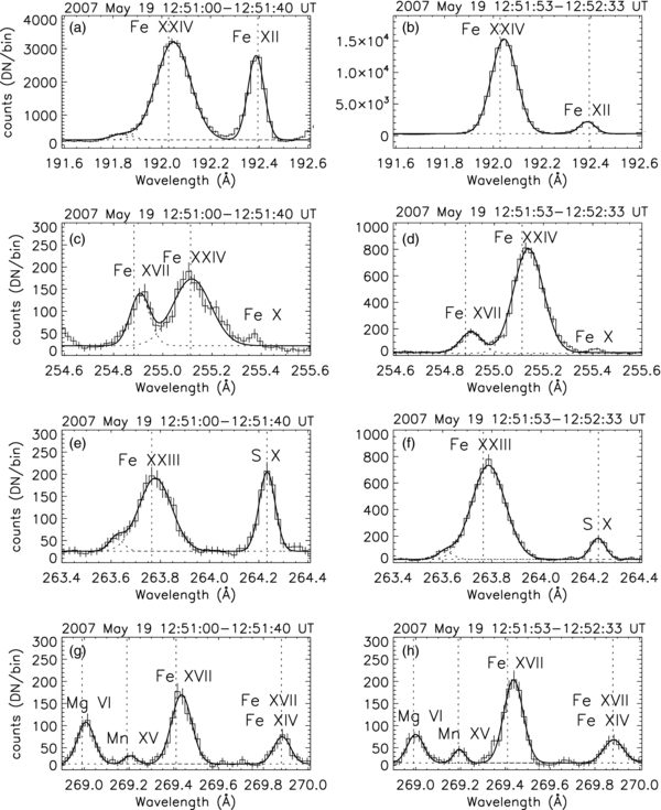
Figure 7. EUV spectra in four wavelength bands at two scanning positions corresponding to two different intervals (12:51:00–12:51:40 UT and 12:51:53–12:52:33 UT). The spatial averages along the EIS slit between two horizontal dotted lines in Figure 5(a) (EW × NS = 1'' × 7'') are applied to observed spectra. Note that the observing point for the Fe xxiv 192 observations is at the east side of that shown in other wavelength ranges by about 2 arcsec. Vertical dotted lines show the wavelength of zero Doppler velocity.
Download figure:
Standard image High-resolution imageIn order to distinguish this blue wing enhancement from potential weak blend lines, we use spectra from the 12:50:06–12:50:46 UT time interval (or at the west position by 1 arcsec), when (or where) the hot line emission is not evident. We show both the Fe xxiii 263 [Fe xxiv 192] spectrum at (X, Y) = (72, 55–61) [(70, 55–61)] or at 12:51:00–12:51:40 UT with a thick line, and the spectrum at the previous scanning point at (X, Y) = (73, 55–61) [(71, 55–61)] for Fe xxiii 263 [Fe xxiv 192] line with a gray line in Figures 8(a) and (b). It is clear that the enhancements have little blend emission at the blue wing. When we select a point, (X, Y) = (70, 50–51), so as not to directly see the S1 bright component, an Fe xxiv 192 Å enhancement above the Fe xiv and Fe xi blend components is evident (Figure 8(c)). Similar line profiles are found in an area extended to the southern part of the hot source S1 as if there is an outflow structure. This observation suggests a reconnection outflow from a site near S1. When we take the difference of the two spectra in Figure 8(c), we can extract a fast flow component of ∼200 km s−1 in the corona (Figure 8(d)). In the same figure, a fast redshift component may be detected, which indicates a downflow of ∼130 km s−1 in Doppler velocity. The radiance of the Fe xxiv blueshift component at (X, Y) = (70, 50–51) is 88 erg cm−2 s−1 sr−1.
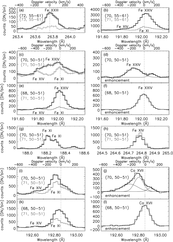
Figure 8. EUV emission-line spectra near the S1 source. (a) Fe xxiii 263 spectra at X = 72, Y = 55–61 (12:51:00–12:51:40 UT), and X = 73, Y = 55–61 (12:50:06–12:50:46 UT), showing no strong blend components at the blue wing of each emission line outside the S1 source. (b) Fe xxiv 192 spectra with the same interval as panel (a) and the same Y positions, but the X positions has an offset of 2 arcsec. Fe xxiv 192 spectra at different positions (c) (X, Y) = (70, 50–51) and (e) (68, 50–51) with (70, 50–51). Panels (d) and (f) display the difference of two spectra in panels (c) and (e), respectively, to reduce the contamination of two blend lines, Fe xi and Fe xiv, in Fe xxiv 192 observations. Panels (i)–(l) are similar to panels (c)–(f) for Ca xvii observations. (g) Fe xi and (h) Fe xiv spectra show that emission lines from the same ions change little at two adjacent areas. Vertical dotted lines show the wavelength of zero Doppler velocity.
Download figure:
Standard image High-resolution imageThe two blended lines near Fe xxiv 192, Fe xiv, and Fe xi in Figure 8(c), must be almost stable at the two adjacent areas because lines from the same ionization states at different wavelengths are also stable at these areas as seen in Figures 8(g) and (h). Hence, there is no possibility that the line shift of blended lines leads to the presence of the additional component. When we look at (X, Y) = (68, 50–51), at 2 arcsec east of the fast flow, the fast outflow component disappears (Figures 8(e) and (f)), suggesting that the fast flows have a width of ∼4 arcsec at least in the X coordinate direction or a short lifetime of a few minutes. Note that the FWHM of the blueshift component (Wobs1) in Figure 8(d) is significantly broader than that in the stationary component (Wobs2) in Figure 8(f) ( = 67.6 km s−1).
When the same method is applied to Ca xvii 192 data as shown in Figures 8(i)–(l), a result similar to that in the Fe xxiv 192 observation (Figures 8(c)–(f)) is obtained. Fast blueshifted flows with velocity up to 400 km s−1 are found at (X, Y) = (70, 50–51) and they disappear at (X, Y) = (68, 50–51). The enhanced component in Figure 8(j) is fitted by three Gaussian functions. There is larger Ca xvii emission at the low Doppler velocity portion in Figure 8(j) compared with the Fe xxiv profile in Figure 8(d). The interpretation of this component is given later.
4.2.2. Spatial Structures of Fast Outflows
It is not easy to make a Doppler velocity map for this flare from hot lines, such as Fe xvii 254/269, Ca xvii 192, Fe xxiii 263, and Fe xxiv 192. The number of detected photons is small for Fe xvii 254/269 and Fe xxiii 263. Ca xvii 192 and Fe xxiv 192 contain blends. In Figure 9, we show an alternative map for the high-velocity component that is seen in the linewidth index of Ca xvii 192. There are blend lines of Fe xiv, Fe xi, and O v lines near Ca xvii 192. When a high-speed flow takes place, the combined emission will have a broad line shape as seen in Figure 8(i). In Figure 9(b), we show the width of a spectral line, which is defined by the width at the level of e−1 for the spectral-line maximum value without fitting a distorted line shape. The white arrow in Figure 9(b) actually shows such features that have a narrow shape in the east–west or X direction as has been mentioned. When we look at the raw line profile, blue-wing enhanced line profiles are found in the area of X = 69–72 and Y = 43–58, whose boundary is shown by a red rectangular box in Figure 10(d) as the area of hot outflow. The outflow can also be identified in the radiance map (Figure 9(a)), which implies that some heating of plasmas takes place there, and that a candidate for the heating mechanism is slow-mode MHD shocks in the Petschek-type magnetic reconnection geometry (Petschek 1964; Cargill & Priest 1982) located above the X-ray flare loop. There are two other enhancements in linewidth: one is near Y = 70, and the other is indicated by a red arrow in Figure 9(b). The former is located at the footpoint region of the flare loops and is due to a stronger contribution of O v 193 that is found at the red wing of Ca xvii 192 and to a contribution of upflow components in Ca xvii 192. The latter might be associated with an erupting structure above the reconnection jet because a blueshifted structure with a similar shape is found in the Fe xv Doppler velocity map (Figure 9(f)).
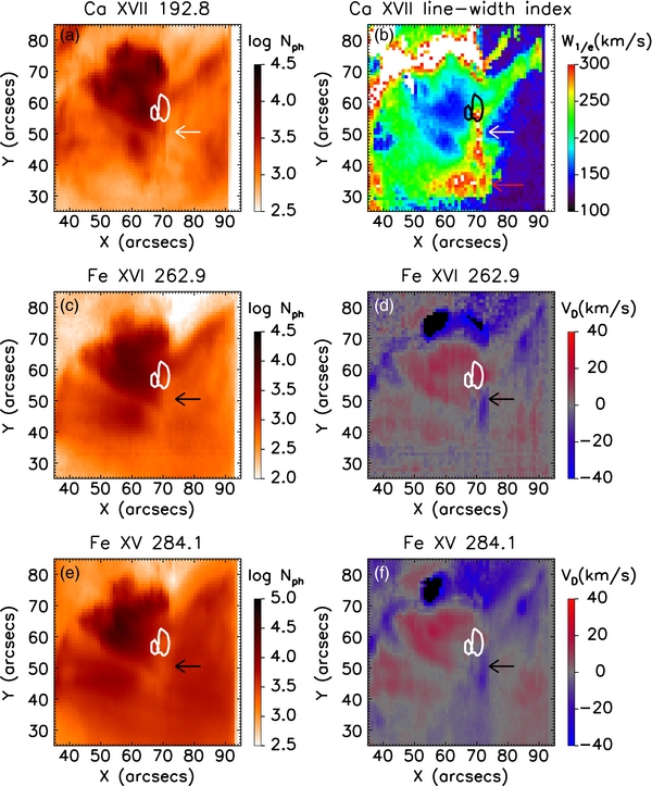
Figure 9. (a) Ca xvii 192 radiance and (b) linewidth index maps. The line profile is significantly distorted from a Gaussian shape in areas showing enhanced linewidth values. The hot outflow is shown by white arrows (−VD = −Vcos i = 200–400 km s−1, where i is the angle between the flow-velocity and line-of-sight vectors). Warm outflows are indicated by black arrows in panels (c)–(f). (c) Fe xiv 262 radiance and (d) Doppler velocity maps. (e) Fe xv 284 radiance and (f) Doppler velocity maps. Contours indicate the Fe xxiii S1 and S2 sources. Unit of radiance here (Nph) is the number of detected photons in an emission line per 1 arcsec2 for exposure time of 40 s.
Download figure:
Standard image High-resolution image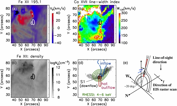
Figure 10. Spatial relationships among (a) Fe xii 195 line-of-sight Doppler velocity VD showing an inflow structure to a site near S1, (b) enhancement in the Ca xvii 192 linewidth index as a signature of hot outflows, and (c) electron density from the intensity line ratio of Fe xii 186/Fe xii 195. (d) Schematic picture of what we see in the EIS velocity observations near the loop-top region with the RHESSI 4–6 keV thermal source at 12:50:30–12:52:30 UT in green contours. (e) Interpretation of observed flows by a geometry of magnetic reconnection viewed from a different perspective.
Download figure:
Standard image High-resolution imageOutflows are also observed in Fe xvi at 262.98 Å and Fe xv at 284.16 Å near the Ca xvii 192 and Fe xxiv 192 hot outflows as shown in Figures 9(d) and (f). The Doppler speed of the flow, which is calculated from the mean wavelength of the line profile with a distorted shape, is −15 km s−1. The broadening of the line profile is observed in the flow with a high-speed component with 150 km s−1 at the blue wing. On the contrary, for the Ca xvii outflow, local enhancement of the radiance is not observed in the Fe xv and Fe xvi outflows as seen in Figures 9(c) and (e), which suggests that these flows are not heated by the process in the flare, but may be pushed out by the flow structure, that is, by the hot outflow. Note that these outflows are seen in the high corona near S1 and that they become visible a few minutes before the appearance of S1. Thus, S1 started to brighten a few minutes after the warm fast outflow began. This suggests that weak magnetic reconnection occurs a few minutes before the impulsive phase. Although remarkable upflow structures of ∼−90 km s−1 are seen in Figures 9(d) and (f) at (X, Y) = (55, 75), we do not discuss these structures here because they appear not to be connected to the S1 source. The line center positions in the bright post flare loops seen in Fe xv and Fe xvi are redshifted and their Doppler velocities are ∼+10 km s−1 near the footpoints.
The vertical alignment of the outflow structure (Figure 9(b)) may be coupled to the EIS slit direction and scanning observation. The perfect alignment of outflow structures to the Y axis at the right or western border of the observed outflow is due to the sudden transition from the pre-flare to flare stage during the slow raster scan. The feature at the left or eastern border of the hot and warm outflows is also nearly aligned to the Y axis. The latter observed feature happens (1) when the projected outflow structure is actually nearly aligned to the north–south direction, or (2) when the wider outflow structure disappears during a short time of a few minutes. In either case, the outflow from a point near the S1 source has the width of at least 4 arcsec in the east–west direction as has been stated in Section 4.2.1.
4.2.3. Te and EM of Fast Outflows
If the fast blueshifted flow is one of a pair of reconnection outflows and if the S1 source is due to plasmas located at the downstream side of the fast MHD shock that is created by the Sun-directed outflow, the temperature of the outflow is expected to be lower than that of the S1 source, because the downstream side is heated by the shock. Although a fast flow is observed at the S1 source as blue-wing enhancement in Fe xxiii 263 and Fe xxiv 192 as shown in Figures 7(a) and (e), the line ratio cannot be used to estimate the electron temperature because the position on the Sun is slightly different between two observations as mentioned before (see Appendix B). When we assume that the outflow plasma observed in Fe xxiv at 192.03 Å and Ca xvii at 192.86 Å moving toward observers is isothermal and in ionization equilibrium, the electron temperature Te and emission measure EM of the outflow component of ∼200 km s−1 Doppler velocity are estimated to be 9.35 ± 0.06 MK and 1.6 ± 0.2 × 1028 cm−5, respectively, from the ratio of the two lines, although the uncertainty of elemental abundance is included. The observation that the temperature of the outflow component is less than that of the loop-top blob is consistent with the following facts: (1) observation of the fast outflow both in Fe xxiv and Ca xvii and (2) no isolated dense structure in Ca xvii at S1, where the hot blob is found in Fe xxiii and Fe xxiv.
4.3. Inflow toward the Site Near the Brightest Fe xxiv/xxiii Source
Figure 10(a) gives the Doppler velocity map from the Fe xii 195 observation showing flows of ∼20 km s−1 in Doppler speed with normal coronal temperatures (∼1.5 MK) toward the hot S1 source. The Fe xii 195 intensity of the inflow at the border of S1 contour is 1.0 × 10³ erg cm−2 s−1 sr−1. A flow structure with the same shape as that of the Fe xii observation is also observed in the Doppler map of Fe x at 184.54 Å. We estimate the line ratio temperature from the intensity of Fe xii at 195.12 Å and Fe x at 184.54 Å. The derived temperature is 1.23 ± 0.02 MK.
The flow was observed at the west side of the S1 source, implying its existence a few minutes before the appearance of the hot source, which has a timing similar to the Fe xv and Fe xvi outflows shown in Figures 9(d) and (f). Although the blueshift structure is located near the west side of the X-ray flare loop structure, they are not the same magnetic structure. An X-ray loop structure that is similar to the flare loop in Figure 10(d) was observed in the pre-flare stage, and it is recognized in the EIS Fe xvi raster-scan map shown by an arrow in Figure 1(f). The loop structure is also seen in Fe xvii and Ca xvii raster-scan maps in Figure 13, but not in Fe xxiii and Fe xxiv maps. The blueshifted flows appear to largely weaken inside the S1 area indicated by a white contour in Figure 10(a), while a part of the hot outflow in the Ca xvii 192 linewidth index (Figure 9(b) or 10(b)) starts within the S1 area. It appears that the inflowing plasmas are heated near S1 and they are flowing out to the outer corona with a higher Doppler speed of a few hundred km s−1.
Figure 10(d) summarizes the spatial relationships with a projection effect among the coronal inflows, the heated hot outflows, the redshifted hot S1 source with a high nonthermal velocity VNT, the flaring loops, and the RHESSI HXR thermal source during the HXR impulsive phase. We suggest that there is a reconnection point near the S1 source at a higher altitude, and that the slow coronal flows are heated and accelerated as the hot reconnection outflow in a geometry of magnetic reconnection as indicated in Figure 10(e). When the system is seen from the line-of-sight direction, the reconnection point is projected to the S1 area, so that the outflow appears to start within S1.
The inflow structure does not show a pair of flows with opposite directivity to a hypothetical reconnection point near the S1 source. Three explanations are possible.
- 1.Line-of-sight integration effect for low-density inflow structure.
- 2.Angle between the direction of flow and line-of-sight direction of the undetected inflow.
- 3.Motion of the diffusion region of magnetic reconnection to the observer.
The third point has been adopted for the spectroscopic observation of reconnection inflow in Hara et al. (2006) from the gradual change of Doppler velocity in the same direction as a function of time near the assumed region of magnetic reconnection.
Figure 10(c) shows the electron density map estimated from the density-sensitive line ratio of Fe xii at 195.12 Å and Fe xii at 186.88 Å, as was done by Young et al. (2009), using the CHIANTI spectral software package (Dere et al. 1997, 2009; Landi et al. 2006). It is apparent that the inflowing structure in blueshift has a low density, while the opposite side of the inflow has a higher density. A footpoint of the X-ray flare loop, which is shown in Figure 10(d), is redshifted and has a high density during the flare decay phase. The electron density in the inflow structure near the S1 source is 2.5 ± 0.5 × 109 cm−3. If the high-density structure shows different Doppler motions, a low-density inflow that is located along the same line-of-sight direction may not be directly detected. Since the fast Ca xvii outflows from the S1 site are only seen for a short duration, the inflow at the opposite side may have disappeared by the time it was reached by the EIS raster scan.
5. DISCUSSION
5.1. Interpretation of Observations by Magnetic Reconnection Process
We have determined the properties that are found at the loop-top region of a long-duration flare. The schematic picture in Figure 11 summarizes the structures of the 2007 May 19 flare site that we have investigated. Multiple flare arcades are formed by the magnetic reconnection process. A local energy release happens in a short time of a few minutes as indicated by the presence of short-lived outflow structures. Although we have not discussed how the flare is triggered, we have shown for the first time all of the relationships among phenomena occurring near the site of magnetic reconnection by means of spectroscopic observations.
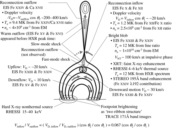
Figure 11. Summary of observations in the present study.
Download figure:
Standard image High-resolution imageWhat we found in the current study is as follows.
- 1.
- 2.Reconnection outflow to the higher corona in Fe xxiii, Fe xxiv, and Ca xvii observations (Figures 8(d) and (j)).
- 3.Outflows of plasmas at the active-region temperature starting a few minutes before the first impulsive-phase HXR peak with little intensity enhancement as a sudden appearance of a flow in the high corona near the site of magnetic reconnection (Figures 9(d) and (f)).
- 4.
- 5.Footpoint HXR emission due to the bombardment of chromosphere by high-energy nonthermal electrons (Figure 5(b)) that appeared at the first HXR peak.
- 6.
- 7.
These observations can be explained by a schematic figure in a framework of the Petschek-type magnetic reconnection process. In order to understand the property of the magnetic reconnection for the 2007 May 19 flare further, we look into the reconnection rate and expected shock structures.
5.2. Reconnection Rate
The Alfvén mach number of the reconnection inflow MA, inflow gives the reconnection rate, and is almost equivalent to the ratio of the inflow speed Vinflow to the outflow speed Voutflow. The Alfvén mach number for the reconnection inflow is calculated as
where VD, inflow, ne, Bc, and θ1 are the Doppler speed, electron density, coronal magnetic field strength, and line-of-sight angle of the reconnection inflow, respectively. The electron density of 2.5 × 109 cm−3 is given from the Fe xii emission-line ratio. The coronal magnetic field strength Bc of 20 G is estimated from the Potential Field Source Surface model (Schrijver & DeRosa 2003) and an assumption that the distance between the top of the flare loop observed with XRT and the line connecting two footpoints is the same as the separation between two footpoints. The extrapolated coronal magnetic field near that height by the potential field approximation is almost horizontal to the line-of-sight direction. MA, inflow is also described by the observed Doppler speed of reconnection outflow VD, outflow as
where θ2 is the line-of-sight angle of the reconnection outflow. If the reconnection outflow originates in the plane that contains the XRT flare loop structure with the shape assumed above, θ2 is about 20 deg (cos θ2 = 0.94). The angle θ1 will be large judging from the geometry, and may be about 60 deg (1/cos θ1 ∼ 2.0). In this case, the MA, inflow value becomes 0.05–0.1, which suggests that Petschek-type magnetic reconnection was actually occurring in the flare site.
5.3. Shock Structures Near the Reconnection Site
The morphology and flows observed in the 2007 May 19 flare are shown in Figure 11. We examine here in greater detail whether the observed plasma parameters support the Petschek-type magnetic reconnection. One way may be to show expected MHD shock structures. The standard reconnection geometry is divided by the MHD shock structures into five regions as shown in Figure 12: (1) inflow region, (2) outflow region in which the direction of outflow is toward the loop structure located below, (3) downstream region of the reconnection outflow, (4) outflow region in which the direction of the flow is away from the solar surface, and (5) hot inflow region that is heated by thermal conduction due to heating at the slow-mode shock. As has been reported above, the reconnection outflow in Region 2 is not found, probably because this region is overlapped with Region 3, where the EUV intensity is much larger than the flow structure.
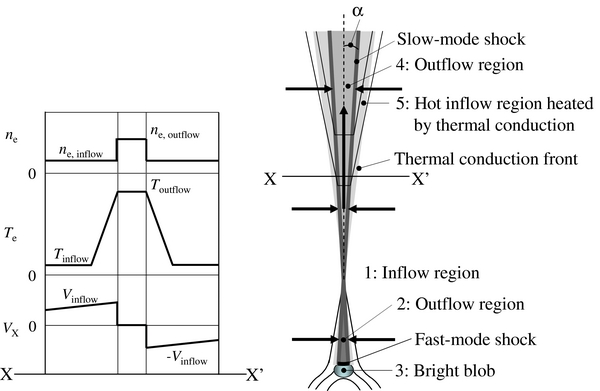
Figure 12. Right: schematic picture of reconnection geometry. Left: model profile in the intersection between X and  in the right panel.
Download figure:
Standard image High-resolution image5.3.1. Slow-mode MHD Shock
The presence of a slow-mode MHD shock structure may be identified by whether or not the plasma parameters meet the jump condition there. The plasma beta β, the ratio of gas pressure to the magnetic pressure, in the inflow region is 0.051, which is estimated from the electron density, electron temperature, and magnetic field strength of the inflow region (ne, 1 = 2.5 × 109 cm−3, Te, 1 = 1.23 MK, and B1 = 20 G). When the inflow plasma is adiabatically heated at the slow-mode MHD shock, the temperature and density ratios that are expected from the Rankine–Hugoniot equations, T4/T1 and ne, 4/ne, 1, are described in terms of β1 as 1 + 2/5β1 and 5(1 + β1)/(2 + 5β1), respectively (Forbes et al. 1989; Aurass et al. 2002). The respective calculated values of these are 8.8 and 2.3 for β1 in our case. The former can be compared with 7.6 ± 0.2 (Te, 4/Te, 1 = 9.35 ± 0.06 MK/1.23 ± 0.02 MK). This observed ratio is equivalent to β1 = 0.061 in the slow-mode shock structure, which is consistent with 0.051, considering the uncertainty of the magnetic field strength in the inflow region.
For a crude estimate of the density ratio at the slow-mode MHD shock, the assumption of the line-of-sight length is required. If the thickness of the outflow region is the same as the width of the X-ray flare loop (w ∼ 4000 km) and the tilt angle of θ2 ∼ 20 deg in the flare loop geometry shown in Figure 10(e), the electron density is estimated to be 3.7 × 109 cm−3, which is higher than that in the inflow region. These ratios provide additional support for the presence of the slow-mode MHD shock in the reconnection geometry that we observed.
5.3.2. Fast-mode MHD Shock
We now discuss the evidence for the existence of the fast-mode MHD shock that is found in the flare impulsive phase as a bright isolated structure at the loop-top region. For simplicity, let us assume that there is an inward or Sun-directed reconnection outflow that has the same temperature as that of the outgoing observed outflow. The temperature ratio Te, 3/Te, 2 ≃ Te, 3/Te, 4 is 1.22 ± 0.02. This temperature ratio is roughly consistent with the value 1.3 in the numerical simulation of Yokoyama & Shibata (2001), which shows that the temperatures of the reconnection outflow and bright blob are ∼9 MK and 12 MK for plasma beta β1 of 0.04 (see Figure 9 in Yokoyama & Shibata 2001).
It is reasonable to assume that the size of the loop-top bright blob in the direction of fast outflows does not significantly exceed the width of the X-ray flare loop (w ∼ 4000 km). In this case, the electron density of the bright blob is 1 × 1010 cm−3 from the emission measure of 4 × 1028 cm−5 in Figure 6(f). Even if we use 10,000 km for the line-of-sight length of the blob structure as an unexpectedly large value, the electron density of the loop-top blob (ne, 3) is estimated to be 6 × 109 cm−3, which is significantly higher than that in the reconnection outflow evaluated above.
In addition to the enhanced highly ionized Fe ion motions in the bright blob with a Sun-directed flow, these observations support the presence of the fast-mode MHD shock that is located just above the bright blob. However, the fast outflow with the Alfvén speed in the inflow region, VA ∼ 870 km s−1 (ne, 1 = 2.5 × 109 cm−3, Bc, 1 = 20 G), is not observed for this flare.
5.3.3. Width of Outflow Region
When the Alfvén speed in the inflow region is 870 km s−1, the angle between two slow-mode shocks 2α in the Petchek-type reconnection geometry (Figure 12) can be calculated from mass conservation between the inflow and outflow as tan α = (Vinflow/VA)(ne, inflow/ne, outflow). Here, α becomes 0.89 deg when values of 20 km s−1, 870 km s−1, 2.5 × 109 cm−3, and 3.7 × 109 cm−3 are used for Vinflow, VA, ne, inflow, and ne, outflow, respectively. The expected width of the outflow region at the point of measurement for Figure 8(j) in the Petchek-type reconnection geometry is calculated as Ltan 2α, and is 530 km for a length L(∼ 8 arcsec/sin θ2) of ∼17,000 km between the reconnection point and the point of measurement for the Figure 8(j) line profile. The width is slightly narrower than the EIS slit width (1 arcsec ∼ 730 km). The convolution of the narrow outflow structure with the EIS spatial resolution of ∼2.5 arcsec cannot completely explain the width of observed outflow (>4 arcsec) that is reported in Section 4.2.1. The warm outflow is located at the west of the hot outflow. If this is regarded as a sign of magnetic reconnection, the width of outflow region in the east–west direction is further extended. Hot outflows might have been observed there a minute later if the same observation had been performed.
In order to reconcile both the expected narrow outflow structure and the observed width of the outflow region, multiple outflow structures side by side above unresolved bright blob structures need to be adopted. This might be consistent with the motion of the thermal HXR sources near the top of the X-ray loop with time as shown by arrows in Figure 18(d), which indicates the multiple magnetic reconnection at different positions. In this case, what we observed with EIS is a mixture of contributions from the hot reconnection outflow (Region 4), a thin slow-mode shock region, and the hot inflow region heated by thermal conduction (Region 5) because these are all observed in an EIS resolution element at the same time.
The density estimate in the high-speed outflow might be slightly higher by a factor of 1.4 (=730/530) than 3.7 × 109 cm−3 because a filling factor of unity is assumed in the estimate. The corrected density ne, 4 is 5.1 × 109 cm−3. The electron density at the bright blob ne, 3 is still higher than the corrected density in the outflow.
5.3.4. Low-velocity Ca xvii Component Near Reconnection Outflow
There is a Ca xvii component showing a low-speed blueshift in Figure 8(j). A similar component was not observed at the same position in the Fe xxiv line profile (Figure 8(d)). Based on these observations and on the Ca xvii line emissivity shown in Figure 13, the temperature of the Ca xvii component is in the range of 4–8 MK. This may reflect the temperature structure near the reconnection outflow. We consider two possibilities.
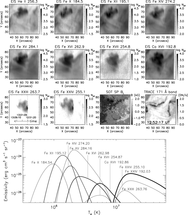
Figure 13. EIS raster-scan images in representative emission lines near the flaring region with the line-of-sight magnetic field strength from SOT SP BL and TRACE 171 Å images. Nph is the number of photons detected with EIS for the exposure duration of 40 s. Logarithmic scale in reverse color is used except for the BL map, while the BL map is shown in linear scale. Emissivity of coronal lines as a function of electron temperature from CHIANTI database is shown at the bottom.
Download figure:
Standard image High-resolution imageOne is a component heated in Region 5 by thermal conduction (Figure 12). As shown in Yokoyama & Shibata (2001), the plasma that is located just outside the slow-mode shock is heated by thermal conduction from hot plasmas heated by this shock. The temperature of the region changes from the outflow temperature to the inflow temperature across the line X–X in Figure 12. In our case, the emission from this region essentially contributes to the Fe xxiv and Ca xvii EUV intensities when the outflow region is not resolved in the observation. The fast flow is not expected here, which is consistent with the low Doppler shift component in the line profile that is seen in Figure 8(j). Since the temperature in the region decreases from that of the slow-mode shock region, with a temperature 9.4 MK, to the inflow region with 1.2 MK, as schematically shown in the left panel of Figure 12, the contribution of the Ca xvii intensity in the region may become comparable to that in the fast outflow because the peak of the Ca xvii contribution function is at ∼5 MK, while the Fe xxiv contribution with a peak contribution function at ∼16 MK rapidly becomes negligible when the temperature decreases from 9 MK to a lower temperature. This can be seen in the contribution functions shown in the bottom panel of Figure 13.
The other is a component in the outflow. In the outflow region, there may be many small-scale magnetic islands or plasmoids that are created in a current sheet as simulated by Shibata & Tanuma (2001) or in multiple current sheets along the line of sight in association with this flare activity. This is the case in which the multiple O-type magnetic structures exist in the reconnection outflow. If the magnetic islands are also heated close to 4–8 MK, the components contribute to the EUV emission that we observe. The map of the Ca xvii linewidth index (Figure 10(b)) shows the presence of non-uniformity in the outflow structure, which in turn supports the existence of small magnetic islands. The structures in the flow may also explain why the Alfvénic flow was not found at the impulsive phase of this flare, because the outflow plus small plasmoids are observed at the same time during the acceleration phase when their combined speed is initially slower than the Alfvén speed of the inflow region.
6. SUMMARY
EIS observed a GOES B9.5 flare on 2007 May 19 during a raster scan. The gradual soft X-ray light curve suggests an LDE with a standard model reconnection geometry, while our observations of the topology of the flare loop show a simple loop structure with characteristics of magnetic reconnection above the loop-top region. The unique feature of the EIS raster-scan observation for this flare comes from the deep exposure for the reconnection region during the impulsive phase, which enables us to investigate the processes occurring near the site of magnetic reconnection.
During the impulsive phase, the brightest source of Fe xxiii and Fe xxiv emission is observed above the top of a soft X-ray flare loop. The presence of Fe xxiii and Fe xxiv ions very early in the flare with emission light curves slightly lagging the RHESSI hard X-rays may indicate direct shock heating in the high corona. A value of VNT ∼ 100 km s−1 or (4–5) × 107 K ion motions is obtained from the Fe xxiii and Fe xxiv profiles for the brightest source that shows an electron temperature of 1.2 × 10⁷ K in the EIS and RHESSI observations during the impulsive phase peak. The maximum Fe xxiii VNT value is seen at the peak of the HXR light curve and then declines rapidly. This rapid decrease may indicate that magnetic reconnection is not progressing steadily. This is supported by the presence of fast outflows from the loop-top region −VD ∼ 200–400 km s−1 in Doppler speed, with a few minutes duration.
A detailed analysis of the line profile in the impulsive phase shows the presence of a collimated high-velocity blueshifted component whose Doppler speed exceeds 200 km s−1. This must be due to reconnection outflow toward the outer corona, though the speed is not high compared with an event shown by Wang et al. (2007). We think that the redshift of the brightest Fe xxiii and Fe xxiv component is a signature of inward-directed flows that were originally faster before colliding with structures below. The outflow temperature is about 9 MK, which is lower than that of the bright blob. A structure inflowing to the brightest region in Fe xxiv 192 is observed in Fe xii 195 with Doppler speed of 20 km s −1. It appeared a few minutes before the impulsive phase. These observations all provide evidence for magnetic reconnection. The reconnection rate (Vinflow/VA) of 0.05–0.1 that is estimated from the observed parameters suggests that Petschek-type fast reconnection was occurring in the flare site.
We further examine whether the observed quantities can support the Petschek-type magnetic reconnection by considering the interface relations at the expected shock structures. The observed temperature ratio at the expected slow-mode MHD shock located between the reconnection inflow and outflow is consistent with the ratio determined from plasma beta estimated in the inflow region, while a density enhancement in the outflow to the inflow region is also derived. These suggest the presence of the slow-mode MHD shock in the flare site. The Ca xvii enhancement in the outflow region has a low Doppler velocity component which is not found in Fe xxiv observations. The candidate for the low-velocity component is a contribution from the inflow region heated by the thermal conduction or from small magnetic islands in the outflow region. The temperature and density of the bright blob are higher than those of the fast outflow. The temperature ratio between the bright blob and the outflow is consistent with the MHD simulation by Yokoyama & Shibata (2001) for a condition of plasma beta that is nearly the same as that estimated from observed parameters. These observations provide supplementary support for the presence of the fast-mode MHD shock located above the bright blob, in addition to the enhanced highly ionized Fe ion motions and the redshift of the bright blob.
The only missing observable is the fast reconnection outflow with the Alfvén speed of the inflow region. A large tilt angle of the outflow to the line-of-sight direction cannot be adopted, because the height of the loop-top region becomes lower. This would result in a stronger magnetic field strength near the loop-top region, which becomes too strong to explain the jump condition in temperature at the slow-mode shock by the reduction of plasma beta in the inflow region. It is likely that the outflow speed is reduced by the obstacle in the current sheet. When magnetic islands such as small plasmoids are contained in the current sheet, the flow speed could be lower than the Alfvén speed in the acceleration phase as shown by Shibata & Tanuma (2001). Non-uniformity of the flow structure in Ca xvii observations may support this view. Note that the observed flow cannot be interpreted as evaporation flow, because the observed outflow starts near the bright blob, which is located in the corona and not on the bright two-ribbon structure near the chromosphere that was observed in TRACE 171 and STEREO 171 observations.
A sit-and-stare observation offers the best way to track the temporal evolution of plasma flows and heating that are associated with magnetic reconnection. However, the probability of detecting a flare in this way is very low. An alternative method for achieving a higher detection probability for flares in an EIS observation would be to perform (1) a continuous raster scan with a narrow scanning range or (2) a sparse raster scan with a periodic spatial interval to speed up the scan time. These studies have already been run for flare-producing active regions after the solar minimum of the Cycle 23, and we will report further from these EIS observations on the site of magnetic reconnection for the observed events.
The authors express appreciation to Dr. Ryan Milligan for his comments on the RHESSI data analysis and to Dr. Shinsuke Imada and Professor Kanya Kusano for discussion on the magnetic reconnection process. Hinode is a Japanese mission developed, launched, and operated by ISAS/JAXA, in partnership with NAOJ, NASA, and STFC (UK). Additional operational support is provided by ESA and NSC (Norway). TRACE, RHESSI, and STEREO are US NASA mission. SOHO is a joint mission of NASA and ESA. This work was carried out at the Hinode Science Center in NAOJ, and was supported by the JSPS Core-to-Core Program 22001. The work of P.R.Y. was performed under a contract with the U.S. Naval Research Laboratory and was funded by NASA.
APPENDIX A: EUV RASTER-SCAN RADIANCE MAPS OF FLARE REGION
Ten selected raster-scan radiance maps from Hinode EIS observations are shown in Figure 13 with the line-of-sight magnetic field strength from Hinode SOT SP observations and the two-ribbon structure in the transition region or the bottom of the corona from the TRACE 171 Å imaging observation. Gray-scale bars are attached to each panel to represent how many photons are detected at each point in the integration time of 40 s. No enhancement is seen in the TRACE 171 Å image at the position of the Fe xxiii or Fe xxiv bright blob, indicating no energy deposition to the chromosphere or transition region at this site. The dotted line in the Fe xxiii 263 radiance map indicates the hard X-ray peak time in the RHESSI light curve for the 12–25 and 25–50 keV energy bands (Figures 6(b) and (c)). The emissivity of each EUV line from the CHIANTI database is shown in the bottom panel of Figure 13 to indicate the range of electron temperature in which each emission line contributes. It is apparent that the sensitivity for detecting hot plasmas is reduced above 8 MK in Fe xvii at 254.87 Å and that the Ca xvii emission feature at 192.86 Å is the unique line for investigation of hot plasmas in the temperature range from 8 to 10 MK. The temperature of the reconnection outflow reported in the present paper is 9–10 MK.
APPENDIX B: EIS SLIT POSITIONS BETWEEN TWO SPECTRAL BANDS
EIS observes in two spectral bands by employing two different multilayer coatings on the primary mirror and concave grating (Korendyke et al. 2006; Culhane et al. 2007). Half the area of each optic is used for the EIS short-wavelength band and the remaining half area is for the long-wavelength band. Thus, EIS consists of two spectrometers sharing the same main optics. Figure 14 shows Fe xi raster-scan radiance maps for the present observation in emission lines located in the EIS short- and long-wavelength bands. The two maps are aligned after taking cross-correlation. Offset values (ΔX, ΔY) of the Fe xi radiance map at 256.93 Å to that at 182.17 Å are (1.7, 17.1) arcsec in this case. The horizontal offset ΔX, which is perpendicular to the slit direction, is caused by the small offset of the solar image on the slit plane due to the two different coatings on the primary mirror. The vertical offset is due to the shift of the solar image on the slit and the positional offset of two CCD detectors. The vertical offset is a function of wavelength as shown by Kamio et al. (2010). This is due to the rotation of grating and CCD around their own normal directions.
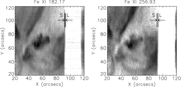
Figure 14. Fe xi emission-line observations (left) at 182.17 Å and (right) at 256.93 Å. Vertical bars show slit positions on the Sun at an exposure for the short- (S) and long- (L) wavelength bands. For two spectral bands, the spectrometer shares the same slit at the focal plane of the EIS primary mirror. White area indicates the eclipse period due to blocking the solar EUV emission by Earth. The distance between two vertical bars is 1.7 arcsec for this observation.
Download figure:
Standard image High-resolution imageNote that the Fe xi emission line at 256.93 Å was thought to be due to Fe xii emission until Del Zanna (2010) identified it. There appears to be a blend line whose formation temperature is close to ∼2 MK at this wavelength, judging from the feature seen near the flare site.
APPENDIX C: LINEWIDTH CALIBRATION FOR THE EIS LONG-WAVELENGTH BAND
The FWHM of emission line Wobs in the EUV spectrum obtained with Hinode EIS includes a contribution due to instrumental origin WI as shown in the following equation:
where WI is the instrumental broadening, k is the Boltzmann constant, Ti is the ion kinetic temperature, Mi is the mass of ion, and VNT is the nonthermal velocity. W is the intrinsic linewidth of solar origin in FWHM.
The pre-launch measurement of the spectral resolution was performed at the Rutherford Appleton Laboratory in 2004 (Lang et al. 2006), and is summarized in Korendyke et al. (2006). This information is not sufficient for calibrating the widths of EIS spectra, because the value of instrumental linewidth is given for only a few wavelengths and at a single off-axis angle. In general, it will be a function both of wavelength and of off-axis position.
Figure 15 shows the FWHM of the Fe xii emission lines at 193.51 and 195.12 Å with an XRT image showing the EIS slit positions. The same trend as a function of EIS CCD-Y height along the slit direction is found for the observed linewidth in Figure 15(c). Since most areas are covered by the quiet Sun, the slow variation of the linewidth as a function of EIS CCD-Y height corresponding to off-axis position is due to the change of instrumental width along the slit direction.
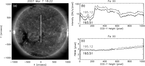
Figure 15. (a) Hinode XRT image on 2007 March 7 with the EIS raster-scan area by a white box that covers 1024 arcsec in the Y direction. (b) Radiance and (c) observed linewidth WI, obs in FWHM for Fe xii emission lines at 193.51 and 195.12 Å are shown as a function of EIS CCD pixel position in the Y direction.
Download figure:
Standard image High-resolution imageFollowing the launch of Hinode, we have measured the EIS instrumental width through a cross-calibration between the on-orbit EIS observation and a coronal spectroscopic observation at a ground-based observatory, Norikura Solar Observatory in the National Astronomical Observatory of Japan. An active region located at the west limb was observed on 2007 July 18 with the two spectrographs by raster-scanning observations. The spectral resolution of the spectrograph at Norikura is λ/Δλ ∼ 105 (Hara & Ichimoto 1999), while it is ∼4000 for EIS. The observations at Norikura were supported by Drs. Y. Suematsu and K. Ichimoto. We used the green line, Fe xiv at 5303 Å, to calibrate Fe xiv lines in the EIS short- and long-wavelength bands. The radiance maps from raster-scan observations are shown in Figure 16.

Figure 16. Co-aligned Fe xiv raster-scan maps obtained during a campaign observation for the calibration of EIS instrumental width. The active region at the west limb was simultaneously observed on 2007 July 18 near 8 UT. The most left is the map from the so-called green-line observation at 5303 Å with dark stripes due to clouds crossing in the field of view and the others are from EIS observations in the short- and long-wavelength bands. The white box in the green-line observation indicates the area where the linewidth is calibrated. For this area, the linewidth is measured as a function of vertical position by averaging horizontal nine raster sampling points.
Download figure:
Standard image High-resolution imageWe assume that linewidths observed with EIS and Norikura spectrographs, Wobs, E and Wobs, N, are expressed by the intrinsic coronal linewidth W and instrumental widths WI, E and WI, N as
and

The EIS instrumental width is estimated from Equations (C2) and (C3). Thus, we obtain WI, E(λ0, Y) as
where λ is a wavelength of Fe xiv lines and Y is a detector position along the EIS slit.
The instrumental width WI, N for the ground-based observation is estimated to be 0.09 Å for a Cr line at 5304.19 Å from the observed Cr linewidth Wobs of 0.13 Å, the thermal width, and nonthermal width. The latter two values are obtained by assuming a photospheric temperature of 6000 K and a nominal value of nonthermal velocity of 3 km s−1. A calculated value, originating from the spectral resolution of the spectrograph, the width of slit, the expected aberration of optics, and the CCD pixel sampling, is 0.06 Å. The observed FWHM of the Fe xiv line at 5302.86 Å is typically 0.8 Å, which corresponds to 45.3 km s−1. When the instrumental width of 0.09 (0.06) Å is removed, the intrinsic FWHM becomes 45.0 (45.1) km s−1. Thus, the effect of instrumental width in our ground-based observation is negligible for the linewidth measurement.
The area enclosed by a white box in the left panel of Figure 16 is analyzed for two Fe xiv emission lines at 264.78 and 5302.86 Å and the results are shown in Figure 17. The top and middle panels in Figure 17 show the radiance in arbitrary units and the observed linewidth in FWHM as a function of the EIS CCD-Y height in the slit direction. When Equation (C4) is applied to the data in the middle panel with WI, N(5303 Å, Y) = 0.09 Å, the instrumental width at 264.78 Å, WI, E(264 Å, Y), is calculated as shown in the bottom panel of Figure 17. There is a trend for the EIS instrumental to increase with the CCD-Y height, which is consistent with the observed linewidth in the quiet Sun (Figure 15(c)). In other words, a non-constant instrumental width as a function of the CCD-Y height needs to be subtracted from the observed linewidth to estimate the intrinsic linewidth W of solar origin.
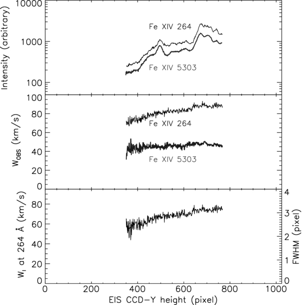
Figure 17. Top: radiance, middle: linewidth, and bottom: EIS instrumental width at 264.78 Å in the white box of Figure 16.
Download figure:
Standard image High-resolution imageThere are Fe xiv emission lines at 252.20, 264.78, 270.52, 274.20, and 288.51 Å. A linear interpolation between 252.20 Å and 264.78 Å is used to evaluate the instrumental width of Fe xxiv (Fe xxiii) at 255.11 (263.76) Å. This is a valid approach because the instrumental width gradually changes in the wavelength direction. The details of the linewidth performance in EIS observations, including the short-wavelength band, will be reported in a separate paper.
APPENDIX D: POSITIONS AND MOTIONS OF RHESSI HXR SOURCES
Figures 18(a) and (b) show the positional relationships among the soft X-ray flare loop, the transition-region brightening observed as a two-ribbon structure, the Fe xxiii bright blob, and the RHESSI thermal and nonthermal hard X-ray sources. The EIS radiance map, XRT, and TRACE images shown here are co-aligned to data in the full-disk observations, and the RHESSI source locations are given from the RHESSI visible-light limb sensors. The HXR local maximum coincides with the location of the EUV bright blob and the local enhancement in the STEREO A difference map (Figure 4(a)). Hence, it appears to be difficult to intentionally move the 15–40 keV source to locate two local maxima on the TRACE two-ribbon structure because the local maximum of the 4–6 keV source is separated from the bright blob at the same time.
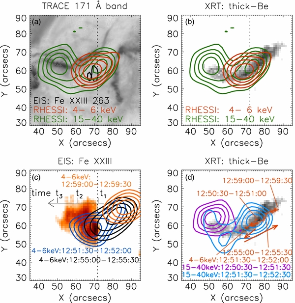
Figure 18. (a) EIS Fe xxiii showing the bright hot source, RHESSI 4–6 keV, and 15–40 keV contours in black, red, and green colors on the TRACE 171 Å image in reverse color. (b) The same RHESSI contours on an XRT image with the thick-Be filter. Integration time of RHESSI data in panels (a) and (b) is two minutes (12:50:30–12:52:30 UT). (c) RHESSI 4–6 keV contours at three different time intervals on EIS Fe xxiii raster. (d) RHESSI 15–40 keV contours at two time intervals in the HXR impulsive phase on the XRT image with centroid positions of RHESSI 4–6 keV HXR sources every 30 s in plus signs. RHESSI contour levels are 60%, 70%, 80%, and 90% of each maximum value.
Download figure:
Standard image High-resolution image
Figure 19. Radiance maps of (a) Fe xiv 257.39, (b) Fe xxiii 263.76, (c) Fe xiv 270.51, and (d) Fe xxi 270.55. (e) Intensity variation in the east–west direction between two dotted lines in panels (b) and (d). Auxiliary vertical lines at X = 70 in panels (b) and (d) visually show that the brightest point in the Fe xxi map is located eastern side to that in the Fe xxiii map.
Download figure:
Standard image High-resolution image
When the integration time (12:50:30–12:52:30 UT) is reduced to one minute by dividing it into two equal time ranges, the nonthermal source at the former half appears at the east, and the source at the latter half does so at the west as shown in Figure 18(d). This implies that a different energy release event was occurring for each time range. The centroid positions of the RHESSI thermal source every 30 s are also shown in Figure 18(d), and were moving along the soft X-ray loop structure in the direction shown by arrows in the panel. It is likely that the successive energy release was occurring by changing the location along the magnetic structure in the corona, resulting in a long-duration flare. The direction of the HXR source motion after the impulsive phase is the same as that of the soft X-ray loops in Figure 2.
APPENDIX E: A FAINT ISOLATED SOURCE IN Fe xxi AT 270.55 Å
A faint isolated source observed in Fe xxi at 270.55 Å (Figure 19(d)) has been found by the subtraction of a much brighter blend line, Fe xiv at 270.51 Å (Figure 19(c)), using a line, Fe xiv at 257.39 Å (Figure 19(a)). The intensity ratio of these Fe xiv lines is constant because the upper atomic level of these transitions is the same. The brightest part of the Fe xxiii structure in Figure 19(b) is located at the west side of the brightest Fe xxi structure in Figure 19(d), which shows that a lower temperature is found at the outer part of the bright blob. There are two possibilities for the Fe xxi structure: one is a temperature gradient in the bright blob, and the other is a cooling of the blob structure by radiation and thermal conduction. When we use the formula of conductive and radiative cooling of Aschwanden & Alexander (2001), the radiative and conductive cooling time scales are 11,000 s and 240 s, respectively, for the temperature of 12 MK, the electron density of 7.5 × 109 cm−3, and the loop half length of 5 × 10⁴ km. Thus, the temperature difference across the bright blob in the east–west direction can simply be explained by conductive cooling.