


ABSTRACT
A B1.7 two-ribbon flare occurred in a highly non-potential decaying active region near a coronal hole at 10:00 UT on 2008 May 17. This flare is "large" in the sense that it involves the entire region, and it is associated with both a filament eruption and a coronal mass ejection. We present multi-wavelength observations from EUV (TRACE, STEREO/EUVI), X-rays (Hinode/XRT), and Hα (THEMIS, BBSO) prior to, during and after the flare. Prior to the flare, the region contained two filaments. The long J-shaped sheared loops corresponding to the southern filament were evolved from two short loop systems, which happened around 22:00 UT after a filament eruption on May 16. Formation of highly sheared loops in the southeastern part of the region was observed by STEREO 8 hr before the flare. We also perform nonlinear force-free field (NLFFF) modeling for the region at two times prior to the flare, using the flux rope insertion method. The models include the non-force-free effect of magnetic buoyancy in the photosphere. The best-fit NLFFF models show good fit to observations both in the corona (X-ray and EUV loops) and chromosphere (Hα filament). We find that the horizontal fields in the photosphere are relatively insensitive to the present of flux ropes in the corona. The axial flux of the flux rope in the NLFFF model on May 17 is twice that on May 16, and the model on May 17 is only marginally stable. We also find that the quasi-circular flare ribbons are associated with the separatrix between open and closed fields. This observation and NLFFF modeling suggest that this flare may be triggered by the reconnection at the null point on the separatrix surface.
Export citation and abstract BibTeX RIS
1. INTRODUCTION
It is well accepted that solar flares, prominence eruptions, and coronal mass ejections (CMEs) are powered by the magnetic free energy stored in the corona prior to the eruption. Storage of free energy requires non-potential magnetic fields, which have large-scale magnetic shear or twist associated with field-aligned electric currents. This energy can build up as a result of the emergence of sheared magnetic fields from below the photosphere (Leka et al. 1996; Schrijver et al. 2005; Schrijver 2007), shearing motions or rotations of the photospheric footpoints (Gesztelyi 1984; Zirin & Wang 1990), and the cancelation of flux in the photosphere (Martin et al. 1985; Livi et al. 1989). To understand when and under which condition a solar eruption will occur, we need to understand the three-dimensional structure of the coronal magnetic configuration prior to the flare. Therefore, modeling of the pre-flare non-potential fields is needed. It is also important to study the evolution of the sheared/twisted magnetic fields prior to the eruption.
Magnetic shear can be observed in many different ways. One method is to study the morphology of Hα filaments and prominences (Schmieder et al. 1996; Martin 1998; Lin et al. 2008). Filaments are located above polarity inversion lines (PILs), which are lines on the photosphere where the radial component of photospheric magnetic field changes the sign. The fine structures of filaments and the underlying filament channels indicate that the magnetic fields in these channels are strongly aligned with the PIL, orthogonal to the direction of the potential fields (Foukal 1971; Martin 1990; Gaizauskas et al. 1997). Large deviation from the potential field can also be observed in photospheric vector fields (Hagyard et al. 1982), and in the corona (Rust & Kumar 1996; Canfield et al. 1999; Moore et al. 2001; Su et al. 2006, 2007a, 2007b; Ji et al. 2008; Huang et al. 2008).
Solar flares can occur in big active regions, small decaying regions, and bright points. Major flares associated with prominence eruptions and CMEs often occur in big active regions around sunspots (e.g., Mandrini et al. 2006). This type of eruption remains a topic of active research, because it can strongly affect our space weather. But these regions are often very complex and difficult to model. The configuration in bright points may be simple, but it is too small to resolve with current instruments. Therefore, flares in small decaying regions should be a good target, because such regions are relatively simple compared to big active regions, and can easily be resolved by current instruments. In the current paper, we select a small decaying region which produced a B1.7 flare on 2008 May 17. This flare is associated with both a filament eruption and CME. The relative size of this flare is "large," because it involves the entire region. The purpose of the paper is to study the build-up of magnetic shear in this region, and to understand its pre-flare magnetic configuration by constructing nonlinear force-free field (NLFFF) models.
2. OBSERVATIONS
2.1. Data Sets and Instruments
On 2008 May 17, a two-ribbon flare occurred in a small decaying active region which is highly non-potential. This flare is observed by STEREO/EUVI (Wuelser et al. 2004) at approximately 10 minute interval with a pixel size of 1 59. The full-disk images at 195 Å and 304 Å are used in this paper. EUV (195 Å) and soft X-ray observations prior to and after the flare are provided by Transition Region and Coronal Explorer (TRACE; Handy et al. 1999) and XRT (Golub et al. 2007; Kano et al. 2008) onboard Hinode (Kosugi et al. 2007). TRACE observed this active region with a field of view (FOV) of 1024'' × 1024'', and the image pixel size is 05. XRT images are taken with Al-poly filter and have FOV of 512'' × 512''. The full-disk line of sight (LOS) photospheric magnetograms obtained by SOHO/MDI (Scherrer et al. 1995) and Global Oscillation Network Group (GONG, Hill et al. 2008) are used to study the evolution of the magnetic fields prior to the flare. The MDI magnetograms we used have a cadence of approximately 96 minutes and a pixel size of ∼2''. The 10 minute cadence GONG magnetograms used in this study have a pixel size of ∼25. The filament information is provided by the full-disk Hα images taken by Big Bear Solar Observatory (BBSO) with a cadence of 30 minutes on May 16. One small FOV Hα image on May 16 from THEMIS is also used.
The vector magnetogram used in this study is taken in MTR instrumental mode by the THEMIS telescope. Multi-spectral ranges were observed simultaneously, we selected two of them for the present work: the doublet of Fe i around 6302 Å and the Hα line. The spectral sampling (spectral resolution) was 0.0125 Å pixel−1 for the Fe i 6302 Å line and 0.0144 Å pixel−1 for the Hα line. The telescope scanned this region from east to west with a step size of 08 from 11:42 to 12:40 UT on 2008 May 16. The spectra were recorded by a 023 pixel size sampling along the slit. At each slit position during the scan, a sequence of six images (I ± Q, I ± U, I ± V) was taken for the measurement of the full Stokes profiles. The raw spectra of THEMIS/MTR were calibrated by spectral de-stretching, dark current subtraction and flat field correction (Bommier & Molodij 2002; Bommier & Rayrole 2002). Then, they were subtracted and added to get the I, Q, U, and V profiles, and fitted by the UNNOFIT inversion codes (Landolfi & Landi Degl'Innocenti 1982; Bommier et al. 2007; Guo et al. 2009) to get the vector magnetic fields.
2.2. Evolution of Coronal Loops and Filaments Prior to and During the B1.7 Flare
A two-ribbon flare (GOES class B1.7) occurred in a small decaying active region around 10:05 UT on 2008 May 17. Figure 1 presents STEREO/EUVI observations of the flare at 195 Å (top row) and 304 Å (bottom two rows) before (Figures 1(a) and 1(d)) and during (other panels) the flare. The separation angle between STEREO A and B was approximately 52° on May 17. The flare morphology is studied mainly based on observations from STEREO B (first two rows), in which this region is close to the disk center. The filament eruption is better observed by STEREO A (last row), in which the region is close to the limb. This figure shows that the flaring active region locates near a coronal hole (marked by white arrows in Figure 1(a)). Two bright quasi-circular ribbons without significant separation motion are observed at both 195 Å and 304 Å during the flare (see Figure 1). By comparison of images before and during the flare, we see that the entire region is involved in the flare.
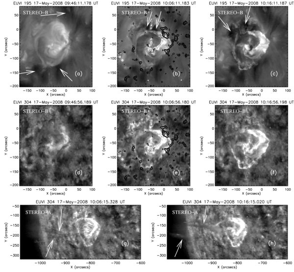
Figure 1. STEREO/EUVI observations at 195 Å (top row) and 304 Å (bottom two rows) of a B1.7 flare on 2008 May 17. (a) and (d) show the EUVI images prior to the flare, and the other panels refer to images during the flare. The white and black contours refer to the positive and negative magnetic fields from SOHO/MDI at 08:03 UT on May 17. Coronal hole is marked with white arrows in (a). The white arrows in (b) and (c) refer to coronal dimmings. The erupted filament material is marked with white arrows in (g) and (h).
Download figure:
Standard image High-resolution imageThe EUV (TRACE) and X-ray (Hinode/XRT) observations prior to (first two columns) and after (third column) the flare are shown in Figure 2. Unfortunately, both TRACE and XRT missed most parts of the flare, during which they were observing another active region on the Sun. Prior to the flare, most of the emission came from two sets of J-shaped loops. In the southern part of the region, a dark lane surrounded by a set of bright J loops was visible in TRACE (Figures 2(a) and 2(b)) for more than 8 hr prior to the flare. This dark lane in EUV could be due to absorption by cool filament material. Corresponding to the EUV dark lane, a fainter dark feature was seen in XRT images (Figures 2(d) and 2(e)). The dark feature observed by XRT probably corresponds to the filament channel due to lack of emission. The two sets of J-shaped loops appear to be highly sheared, because the angles between the lines connecting the footpoints of these loops and the underlying PIL are very small. The underlying PIL information is provided by the dashed black line for the northern loops and dark lane for the southern loops. Note that even potential loops may appear as a J shape in projection to the image plane. However, these loops are confirmed to be highly non-potential by comparison with a potential field model.
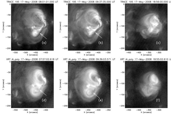
Figure 2. TRACE (top panels) and Hinode/XRT (bottom panels) observations of the region before (first two columns) and after (third column) the B1.7 flare on May 17. The black dashed line in (a) represents the locus of the filament. The dark lane in TRACE and XRT images are marked by white arrows.(An animation of this figure is available in the online journal.)
Download figure:
Standard image High-resolution imageIn TRACE, the pre-flare loops began to rise slowly around 09:30 UT (see online video 1). At 09:54 UT, bright filament material was ejected toward the south then to the east followed by appearance of bright flare ribbons. The escape of filament material was clearly seen at 304 Å by STEREO-A (see Figures 1(g) and 1(h)). The pre-flare loops became invisible around 10:04 UT, when coronal dimming (see Figures 1(b) and 1(c)) was observed at 195 Å in the northeastern part of the region. After the flare, the J-shaped pre-flare loops were replaced with nearly potential loops (Figures 2(c) and 2(f)) between the negative leading polarities and the main positive polarities. We state that these post-flare loops are nearly potential, because they appear to be nearly perpendicular to the underlying PIL. Comparison with a potential field model further confirms this statement. We also find a shrinking of the region by comparison of the pre-flare (first two columns) and post-flare images (third column) in Figure 2. The entire region was enclosed within a coronal hole after the flare, while only three sides of the region were surrounded by the coronal hole before the flare. This indicates that part of the closed fields (overlying the filament) are opened during the flare. This flare was also associated with a CME, which first appeared at 10:15 UT in STEREO-A/COR1 and at 10:36 UT in LASCO/C2.
2.3. Evolution of the Coronal Loops Surrounding the Southern Filament
To understand the formation of the highly sheared pre-flare loops, we study the coronal evolution during a 24 hr period prior to the flare. Small ejections followed by brightenings of different loops frequently occurred in the northern part of the region, but no significant magnetic field reconfiguration was observed (TRACE and STEREO). On the other hand, significant evolution was found in the southern loop system. At 11:42 UT on May 16, THEMIS observed two filaments in this region. The southern filament was long and dark, while the northern one was wide, as shown in Figure 3(a). Later on, the southern one disappeared rapidly, while the northern one became dark (see Figure 3(c)). The TRACE observed several bright sheared loops corresponding to the northern filament, as well as a small bright point consisting of several small loops near the southern end of the sheared loops, as shown in Figure 3(b). Corresponding to the southern Hα filament, the TRACE saw a mixture of bright and dark features. We call the dark features filaments, and the bright features are called loops (or hot filaments). Figure 3(b) also shows two short sheared loop systems (i.e., Loops 1 and Loops 2) corresponding to the southern filament around 12:42 UT on May 16.
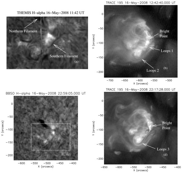
Figure 3. Hα (left column) and TRACE/EUV (right column) observations prior to and after a filament eruption on May 16. The field of view of (a) is approximately 158'' × 102'' (688 × 442 in pixels). The white box in (c) refer to the FOV of (a).
Download figure:
Standard image High-resolution imageAround 20:15 UT on May 16, the TRACE and STEREO observed small ejections followed by brightenings of different sheared loops occurring in the northern part of the region. In the mean time, bright filament material in the southern end of the region started to eject toward the east. Consequently, the two short loop systems corresponding to the southern filament evolved into several long J-shaped loops (i.e., Loops 3) as shown in Figure 3(d). These southern long J loops remained until the occurrence of the B1.7 on May 17. A similar observation of two soft X-ray loops linking into a single sigmoid observed by Yohkoh has been reported by Pevtsov et al. (1996). One interpretation is that the sigmoid is formed due to the "linkage" through convergence and cancelation of the magnetic field of two previously unconnected dipoles (Martens 2003).
In addition to the small ejections of bright filament material in the southern filament channel around 20:15 UT on May 16, the STEREO and TRACE also observed dark filament material in the northern filament channel gradually flowing toward the east. Several bright loops appeared in the southeastern part of the region as shown in Figure 4. No bright loops were clearly visible in the southeastern part of the region around 11:46 UT (Figure 4(a)). One or two bright loops became visible around 20:36 UT (Figure 4(b)). At 00:06 UT on May 17, three bright loops (marked by white arrows) were clearly seen by EUVI, as shown in Figure 4(c). These loops are confirmed to be highly non-potential by a comparison with a potential field model. The appearance of these loops may be evidence of an extension of the southern filament channel. The formation of the southeastern loops was clearly visible in EUVI (STEREO-B), but not in the TRACE. This may be due to projection effect, because this region is close to the disk center in view of STEREO-B, but further away from the disk center as observed in the TRACE.
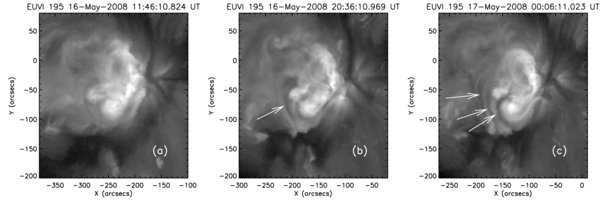
Figure 4. Formation of bright loops (marked by white arrows) in the south eastern part of the region observed by STEREO/EUVI.
Download figure:
Standard image High-resolution image2.4. Evolution of Photospheric Fields
The photospheric magnetic field of this active region was evolving between May 16 and 17. A series of magnetograms during a 24 hr period before the B1.7 flare are shown in Figure 5. Figure 5(a) shows the vector magnetogram observed by THEMIS at 11:42 UT. The white bars refer to the observed transverse field without 180° ambiguity resolution. Figures 5(b)–(d) show the LOS magnetograms from SOHO/MDI. Two LOS magnetograms from the GONG are shown in Figures 5(e) and 5(f).
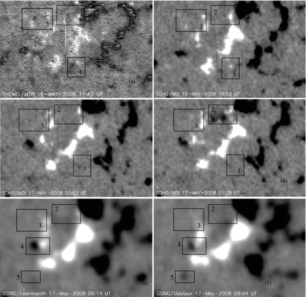
Figure 5. Evolution of magnetic fields observed by THEMIS, MDI, and GONG on May 16 and 17. (a) Vector magnetogram observed by THEMIS at 11:42 UT. The vectors refer to the observed vectors without 180°-ambiguity resolution. (b)–(d) Line-of-sight magnetograms observed by SOHO/MDI at different times on May 16 and 17. (e) and (f) LOS magnetograms from GONG at different times on May 17. The white and black spots in each panel refer to positive and negative polarities. The FOV of each panel is approximately 158'' × 102''. The saturation levels of each image are 100 Gauss (maximum) and −100 Gauss (minimum).
Download figure:
Standard image High-resolution imageFlux emergence and cancelations frequently occurred in different areas (enclosed by black boxes in Figure 5) of the region. A comparison of Figures 5(b) and 5(c) suggests a flux cancelation in the small bipole enclosed by box 1. This may be associated with the filament eruption followed by the formation of southern long J loops around 20 UT on May 16. This observation suggests that these long J loops may be formed through the "linkage" of the magnetic field of two previously unconnected dipoles as mentioned in Section 2.3. Flux emergence (Figures 5(c) and 5(d)) in box 2 occurred early on May 17 may be associated with the frequent filament ejections in the bright point marked in Figure 3. A comparison of Figures 5(a) and 5(c) shows that small polarities enclosed by box 3 in Figure 5(a) are also canceled. All of the aforementioned activities appear not to be directly related to the B1.7 flare on May 17, since they occurred several hours prior the flare. A comparison of Figures 5(e) and 5(f) shows flux cancelations (e.g., in boxes 2 and 4) and emergence (e.g., in box 5) that may be relevant to the flare. The 10 minute cadence GONG magnetograms show that these flux activities started at least three hours before the flare and continued throughout the flare. Higher resolution and higher polarimetric sensitive magnetograms would be certainly useful to clarify these points. The timescale of the evolution of magnetic field triggering flares is commonly hours and not minutes. Unfortunately, THEMIS was not observing on May 17 due to clouds.
3. MAGNETIC FIELD MODELING
The observations discussed in the previous section indicate that the coronal magnetic field in this decaying active region deviates significantly from a potential field. Sheared and/or twisted fields can exist only in parts of the corona where the magnetic field is closed, i.e., field lines are anchored in the photosphere at two ends. The EUV and X-ray images of this region show that the region is surrounded by coronal holes on three sides, so the closed-field region likely extends only to limited height in the corona (h ∼ 0.1 R☉, comparable to the size of the region). Prior to the flare non-potential fields are present throughout this closed-field region, and during the flare the entire region is involved in the event. It is not clear how such a small decaying active region can develop such a strong deviation from the potential field.
To understand how magnetic shear builds up in this region, we develop NLFFF models of the region for two different times (2008 May 16 at 11:42 UT and May 17 at 8:03 UT). The models are constructed by inserting a weakly twisted flux rope into a potential field and then allowing the field to relax to a force-free state using magneto-frictional relaxation (van Ballegooijen 2004). The flux rope insertion method is different from other methods (e.g., DeRosa et al. 2009; and references therein) for reconstructing the NLFFFs by extrapolating observed vector fields into the corona. The method only requires the radial component of the magnetic field in the photosphere, and therefore is less affected by errors in transverse field measurement. A detailed description of the flux-rope insertion method can be found elsewhere (Bobra et al. 2008; Su et al. 2009) and will not be repeated here.
The models we constructed are based on vector magnetograms from THEMIS and LOS magnetograms from SOHO/MDI, and are further constrained by the shapes of coronal loops seen in the TRACE, Hinode/XRT, and STEREO images. The models are force-free in the corona, but take into account non-force-free conditions in the photosphere (Metcalf et al. 1995) as described in Section 3.1. The force-free condition implies that electric currents flow parallel to the field lines, ∇ × B ≈ αB, where B(r) is the magnetic field and α(r) is the torsion parameter, which is constant along field lines. The force-free approximation is reasonable in the corona of active regions up to height of 0.2 R☉ above the photosphere (Gary 2001) because the magnetic pressure is much larger than the gas pressure.
In Section 3.1, we first describe how the THEMIS and MDI magnetograms are combined to provide the lower boundary condition for the three-dimensional (3D) magnetic models, and then briefly describe how the models are constructed. In Section 3.2, we describe the modeling results.
3.1. Modeling Approach
The 3D magnetic models constructed here include not only the active region itself, but also part of the surrounding coronal holes where the magnetic field is open. The reason is that magnetic shear can only build up in the closed-field part of the active region, and the size of this region is strongly affected by the surrounding open fields. We consider a wedge-shaped volume extending from the solar surface (r = R☉) to r = 1.54 R☉, where the field is assumed to be radial. The magnetic field B(r) in this volume is computed on a spherical grid with variable grid spacing.
The first step in the modeling is to specify the radial component of the magnetic field at the lower boundary of the computational domain, Br(R☉, λ, ϕ), where ϕ and λ indicate longitude and latitude on the Sun. The radial field is computed from magnetograph data. For regions outside the THEMIS FOV, the radial field is given by Br = B∥/cos θ, where B∥ is the LOS magnetic field from MDI, and θ is the heliocentric angle. This method assumes that the magnetic field on the Sun is more or less radial, which is reasonable outside sunspots. A similar approach is used inside the THEMIS FOV for cells where the strength |Bobs| of the magnetic field observed by THEMIS/MTR is less than 50 G. The full magnetic vector is used only in cells where |Bobs|>50 G. The observed magnetic vectors are subject to the usual 180° ambiguity in the azimuth angle of Bobs with respect to the LOS. Detailed descriptions of the ambiguity resolution method can be found in the appendix.
The gray-scale image in Figure 6 shows the radial magnetic field Br in the photosphere as a function of longitude and latitude on the Sun (white for Br > 0, black for Br< 0). The vectors show the observed vector field in the local reference frame. The white lines ending with two circles refer to the selected filament path along which the flux rope is inserted. The region with vectors in Figure 6(a) refers to the radial field derived from THEMIS, while other parts are from MDI. Figures 6(b) and 6(c) show the zoomed view of two regions enclosed by white and black boxes in Figure 6(a). The vectors are the vectors after 180° ambiguity resolution. For the region at 11:42 UT on May 16, we inserted two flux ropes corresponding to the two filaments, while three flux ropes are inserted at 08:03 UT on May 17. The field is relaxed to a force-free state using magneto-frictional relaxation (Bobra et al. 2008; Su et al. 2009). This is done by evolving the MHD induction equation while an upward force is applied in the photosphere. The purpose of this force is to simulate the effects of magnetic buoyancy on photospheric magnetic elements (Metcalf et al. 2008; Bobra et al. 2008). Therefore, the NLFFF model constructed here is force free only in the region above the photosphere, and in the photosphere the field has been modified by the effect of the buoyancy forces.
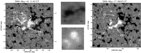
Figure 6. (a) Magnetic map of the decaying active region on 2008 May 16 at 11:42 UT derived from THEMIS and SOHO/MDI data. (b) and (c) Zoomed regions enclosed by white and black boxes in (a). The vectors show the horizontal components of the observed magnetic field after ambiguity resolution. The vectors are plotted in black or white depending on whether the background is light or dark. The maximum horizontal fields in (b) and (c) are 98.6 G and 51.6 G, respectively. (d) Magnetic map of the region on 2008 May 17 at 08:03 UT derived from MDI data. The gray-scale images in each panel show the radial magnetic field Br in the photosphere as function of longitude and latitude on the Sun (white for Br > 0, black for Br < 0). In panels (a) and (d), the white lines ending with two circles refer to the selected filament paths along which flux ropes are inserted.
Download figure:
Standard image High-resolution image3.2. Modeling Results
3.2.1. Best-fit NLFFF Model Selection
For this decaying active region at two different times prior to the B1.7 flare, we construct a grid of NLFFF models with different values of axial and poloidal fluxes of the flux rope. Potential field models are also constructed for comparison. Some of the models we construct converge to a NLFFF equilibrium state, while others do not converge and the flux rope lifts off. Such "lift-off" occurs when the overlying coronal arcade is unable to hold down the flux rope in an equilibrium state, which happens when the axial and/or poloidal fluxes exceed certain limits. This lift-off is a result of the "loss of equilibrium" of the magnetic system, and is not a numerical problem. Therefore, stable NLFFF exists only when axial and poloidal fluxes are below certain limits.
We determine the best model based on the following criteria: (1) this model should best fit the observed highly sheared loops, and (2) this model should converge to a stable solution.
To constrain the model at 11:42 UT on May 16, we select two coronal loops observed by the TRACE (red lines in Figure 7(a)). The model at 08:03 UT on May 17 is constrained by five coronal loops, including two loops (red lines) from the background XRT image in Figure 7(c), and three loops from the STEREO image at 00:06 UT on May 17 (Figure 4(c)). The axial flux (Φaxi) and poloidal flux (Fpol) of the flux ropes for three best-fit models are shown in Table 1. Model 1 is the best-fit model at 11:42 UT, while models 2 and 3 are two best-fit models with different numbers of flux ropes at 08:03 UT. The blue and light blue lines in Figure 7(a) are the corresponding best-fit model field lines from model 1 for the two TRACE loops. The method of finding the best-fit model field lines can be found in Su et al. (2009). For the two XRT loops in Figure 7(c), the closest blue and light blue field lines are the corresponding best-fit model field lines from model 3, and the other blue and light blue lines as well as the pink line in Figure 7(c) are the best-fit model field lines for the STEREO loops in Figure 4(c). Figures 7(a) and 7(c) indicate that the model field lines match the observed loops very well. The dips (yellow) of model field lines for models 1 and 3 overlying on the corresponding Hα images are shown in Figures 7(b) and 7(d). The dips also show a good fit to the observed filament.

Figure 7. NLFFF models on May 16 at 11:42 UT (first row) and May 17 at 08:03 UT (second row). The red and green contours refer to positive and negative magnetic fields from THEMIS+MDI (first row) and MDI (second row). The grey scale images in (a) and (c) are TRACE image at 12:42 UT on May 16 and XRT image at 09:36 UT on May 17, respectively. The grey scale image in (b) and (d) are the Hα images at 11:42 UT (May 16, THEMIS) and 00:21 UT (May 17, BBSO). The red lines in the first column refer to selected coronal loops observe by TRACE or XRT. The pink, blue, and light blue lines are the best-fit model field lines. Dips of model field lines (yellow) are shown in the second column.
Download figure:
Standard image High-resolution imageTable 1. Parameters for Three NLFFF Models
| Flux Rope | 2008 May 16 11:42 UT | 2008 May 17 08:03 UT | ||||
|---|---|---|---|---|---|---|
| Model 1 | Model 2 | Model 3 | ||||
| Fpol | Φaxi | Fpol | Φaxi | Fpol | Φaxi | |
| 1 | 1 × 10¹⁰ | 7 (15) × 1019 | 1 | 7 (15) × 1019 | 1 | 7 (15) × 1019 |
| 2 | 0 | 7 (15) × 1019 | 0 | 15 (20) × 1019 | 0 | 15 (20) × 1019 |
| 3 | 0 | 15 (20) × 1019 | ||||
Notes. Models 1 and 2 contain two flux ropes, and model 3 contains three flux ropes. The poloidal flux (Fpol) and axial flux (Φaxi) of the flux rope are in units of Mx cm−1 and Mx, respectively. The upper limit of the axial flux of the flux ropes is given in brackets.
Download table as: ASCIITypeset image
Figure 8 shows maps of a quasi-separatrix layer (QSL, Demoulin et al. 1996) for models 1 (Figure 8(a)), 2 (Figure 8(c)), 3 (Figure 8(d)), and a potential field model (Figure 8(b)) at 08:03 UT. The open field region is indicated in yellow, while the field lines in the blue area are closed. The boundaries between the blue and yellow areas are the separatrix surfaces between closed and open field regions. The white lines within the blue area are the quasi-separatrix layers, which indicates where rapid changes in footpoint connectivity occur. The white lines ended with two circles refer to the filament paths where the flux ropes are inserted.
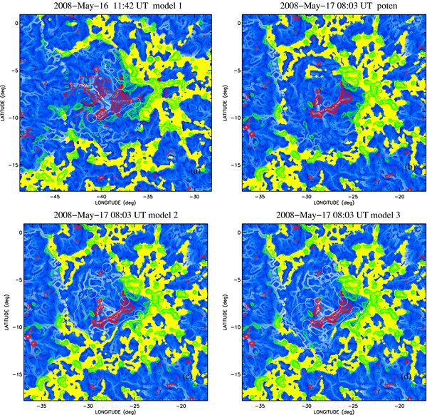
Figure 8. QSL maps at height of 1 Mm for different models. (a) NLFFF model at 11:42 UT on 2008 May 16. (b)–(d) Potential field model, NLFFF model with two flux ropes, and NLFFF model with three flux ropes at 08:03 UT on 2008 May 17. The open field region is indicated in yellow, while the field lines in the blue area are closed. The white layers are the QSLs. The red and green contours refer to positive and negative magnetic fields. The white line ending with two circles refers to the selected filament path along which the flux rope is inserted.
Download figure:
Standard image High-resolution imageAs discussed in Section 2, prior to the filament eruption on May 16, the TRACE (two short bright loop systems) and MDI (existence of a small bipole in Box 1 of Figures 5(a) and 5(b)) observations suggest that the southern filament may be two short filaments. Therefore, for the region on May 16, we construct models with two types of path selection (two short paths, and one long continuous path) for the southern filament. We find that the model with a continuous path is slightly better than the model with two paths. Moreover, there are no significant differences between these models. Therefore, the model with a continuous path for the southern filament (model 1, Figure 8(a)) is used in the current paper. A rough comparison of Figures 8(a) and 8(b) with Figure 1(b) suggests that the outer flare ribbon is closely associated with the separatrix between open and closed fields in model 1 and the potential model at 08:03 UT. The observations discussed in Section 2.3 suggest that the southern filament channel may be extended after the filament eruption on May 16. Therefore, we construct a series of NLFFF models with a longer southern flux rope at 08:03 UT on May 17 (see Figure 8(c)), and the best-fit model is model 2. As compared with Figure 1(b), Figure 8(c) shows that the outer flare ribbon in the southern part of the region is located in the open field region. This conflicts with flare theory which assumes that the flare is caused by reconnection of originally closed magnetic fields. So, we change the southern filament path into two shorter paths (see Figure 8(d)), then construct a grid of NLFFF models. The flux rope paths and QSL map for the best-fit model (i.e., model 3) are shown in Figure 8(d). The outer flare ribbon in Figure 1(b) is close to the separatrix of the open and closed field regions in model 3 (i.e., boundary between blue and yellow areas in Figure 8(d)). Hence, we think that model 3 is the best-fit model at 08:03 UT. This study shows that the comparison of QSL maps with flare ribbons could also be used to constrain the model.
3.2.2. Comparison of NLFFF Models on May 16 and 17
Figure 9 shows front (first column) and side (second column) views of selected model field lines from model 1 (first row) and model 3 (second row). The best model at 11:42 UT on May 16 (i.e., model 1) is well converged, and the axial flux of the flux rope is well below the upper limit which is shown in Table 1 (in brackets). The axial flux of the northern flux rope for the best model (i.e., model 3) remains the same at 08:03 UT on May 17, while the axial flux in the southern flux rope is much larger and not far from the upper limit. Moreover, model 3 is marginally stable.
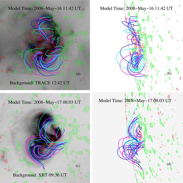
Figure 9. Front (first column) and side (second column) views of NLFFF models with selected field lines on May 16 at 11:42 UT (first row) and May 17 at 08:03 UT (second row). The red and green contours refer to positive and negative magnetic fields from THEMIS+MDI (first row) and MDI (second row). The gray-scale images in (a) and (b) are TRACE images at 12:42 UT on May 16 and XRT images at 09:36 UT on May 17, respectively.
Download figure:
Standard image High-resolution imageAt 11:42 UT on May 16, our model (model 1) suggests that this region contains two weakly twisted flux ropes held down by overlying potential field lines, as shown in Figure 9(a). The relative height of the field lines in Figure 9(a) can be seen in Figure 9(b). Our best model at 08:03 UT (model 3) on May 17 shows that this region contains three weakly twisted flux ropes with fewer overlying potential field lines, see Figure 9(c). The magnetic configuration at 08:03 UT has higher non-potentiality than that at 11:42 UT, which can be found from a comparison of Figures 9(a) and 9(c).
The increase of axial flux in the southern flux rope appears to be related to the flux cancelation (of the small bipole enclosed in box 1 of Figure 5) near the PIL on May 16, as shown in Section 2.4. Canceling magnetic fields have been observed to be related to flares and filament formations (Martin & Livi 1992, and references therein). The observed cancelation of the magnetic flux can be interpreted as a result of magnetic reconnection which concurrently leads to the disappearance of LOS magnetic flux near the photosphere and to the building up of a mostly horizontal filament magnetic field in the corona (van Ballegooijen & Martens 1989).
3.2.3. Comparison of Vectors in Different Models and Observations at Different Layers
Figure 10 shows the magnetic field in small zoomed regions from the potential field model and the best NLFFF model (i.e., model 1) at 11:42 UT on May 16. The gray-scale images show the radial component of the magnetic field, and the vectors show the horizontal components. Both the vectors and gray-scale images are shown in the heliographic coordinates. The first and second columns show observed (blue) and modeled (black and white) vectors from the two ends of the southern flux rope (S1 and S2 in Figure 6(a)) at photosphere. These two columns show that there is a difference between the observed and modeled vectors at the photospheric level. However, this difference is no more than 50 gauss, which is close to the measurement uncertainties. Note that some observed vectors are in the opposite direction compared to the modeled ones. Because they are in the heliographic coordinates, even if the horizontal components are opposite, the observed vectors we choose are closer to the modeled vectors (potential model) than the other solution of the 180° ambiguity. The first two columns of Figure 10 also show that there is no significant difference between the potential field model and the NLFFF model at photosphere. However, there is a clear difference between these two models at chromosphere (height ∼2 Mm) as shown in the third column of Figure 10.
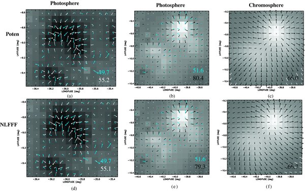
Figure 10. Vectors in small zoomed regions from the potential field model (first row) and the best-fit NLFFF model (second row) at 11:42 UT on 2008 May 16. The regions in the first and second columns are corresponding to regions S2 and S1 as marked in Figure 6(a). The first and second columns show modeled (white or black) and observed (blue) vectors at photosphere. The third columns show the modeled vectors at chromosphere for region S1. The maximum horizontal field strength in the unit of Gauss is shown at the lower right corner of each panel.
Download figure:
Standard image High-resolution image4. DISCUSSION
There are basically three alternatives for triggering solar eruptions: internal tether cutting, external tether cutting ("break out"), and ideal MHD instability or loss of equilibrium (Moore & Sterling 2006).
For some flares flux emergence and cancelation along the PIL are important for tether cutting. Reconnection occurring below or within the flux rope may lead to internal tether cutting (Moore et al. 2001), and such reconnection may be associated with photospheric flux cancelation (van Ballegooijen & Martens 1989). For our case, GONG mangetograms show evidence of flux emergence and cancelations that may be related to the flare.
For some other flares, there is reconnection in high corona, and the overlying loops are removed, e.g., the "break-out" model (Antiochos et al. 1999). The key new feature of the break-out model is that the CMEs occur in multipolar topologies in which reconnection between a sheared arcade and neighboring flux systems triggers the eruption. In this break-out model, reconnection removes the unsheared field above the low-lying, sheared core flux near the neutral line, thereby allowing this core flux to burst open (Antiochos 1998). The magnetic configuration prior to the B1.7 flare on May 17 is a bipole surrounded by open fields on three sides, which is different from the multipolar topology in the break-out model.
On the other hand, eruptions may also occur due to a catastrophic loss of equilibrium or catastrophe (Forbes & Isenberg 1991; Isenberg et al. 1993; Lin & Forbes 2000). In this model, energy is stored in the corona as the flux rope system evolves quasi-statistically through a set of equilibrium states until a point is reached where equilibrium is no longer possible. At this point, a catastrophe occurs and the flux rope erupts. Our NLFFF modeling suggests an increase of axial flux occurred prior to the flare. The best-fit NLFFF model prior to the flare is in a marginally stable state. These results suggest that the onset of the flare may be due to the loss of equilibrium.
Our NLFFF model prior to the flare shows that a magnetic null exists at a height of 25 Mm in the corona, as shown in Figure 11(a). Associated with this null is a fan surface that separates open and closed fields, and a spine that passes through the null (Priest 1996). Such a null also exists in the potential field model. Actually, the null point is more like a line of nulls that is oriented in the southwest direction relative to the true null (see Figure 11(a)). This is due to the asymmetric distribution of magnetic flux below the null point. However, on a larger scale the separatrix surface is more or less axisymmetric. A cartoon of the pre-flare configuration in two dimension is shown in Figure 11(b). The magnetic configuration prior to the flare can be divided into three parts: (1) the inner part is low-lying highly sheared field located just above the PIL (shaded region in Figure 11(b)), (2) the envelope field immediately coating the sheared core field is closed and unsheared, and (3) the outermost part is open field. The magnetic null is marked as a star sign in Figure 11(b).

Figure 11. (a) Selected field lines (from model 3) showing the separatrix surface between open and closed fields, and the magnetic null at height of 25 Mm. It is a 3D plot projected on the 2D plane. (b) A cartoon that illustrates the 2D view of magnetic configuration prior to the flare. The shaded area refers to the highly sheared core fields.
Download figure:
Standard image High-resolution imageThis configuration is like a dipole embedded in a uniform background as shown in Antiochos (1998) and Pariat et al. (2009). Therefore, another plausible scenario for our B1.7 flare is the one proposed by Pariat et al. (2009) for polar jets. The key idea underlying this model is that the magnetic configuration is nearly axisymmetric, and that reconnection is forbidden for an axisymmetrical null-point topology. Consequently, by imposing a twisting motion that maintains the axisymmetry, magnetic stress can be built up to high levels until an ideal instability breaks the symmetry and leads to an explosive energy release via reconnection. Prior to the B1.7 flare, the system stayed close to axisymmetry, and free energy slowly built up in the corona (likely by flux cancelations), which is found from both observations and modeling. Beyond a certain critical twist/helicity, the approximately axisymmetrical system became unstable to a 3D kink-like mode that broke the symmetry and immediately induced pervasive reconnection in the null point. This reconnection removed the overlying unsheared field above the low-lying, sheared core flux near the neutral line, thereby allowing this core flux to burst open. This model is also consistent with our observations that the flare ribbons are closely associated with the separatrix between open and closed fields.
5. CONCLUSIONS
We carry out a comprehensive observational and NLFFF modeling study on the evolution of magnetic configuration prior to a B1.7 flare on 2008 May 17. Two bright quasi-circular ribbons without significant separation motion were observed during the flare. This flare occurred in a small decaying active region surrounded by a coronal hole on three sides. The flare is "large" in the sense that it involved the entire active region, and a filament eruption and CME are associated.
This active region contained two filaments around 11:42 UT on May 16. Following a filament eruption around 20:00 UT, the two short loop systems corresponding to the southern filament evolved into one long highly sheared loop system. This evolution appears to be associated with flux cancelations in a small bipole close to the southern PIL. Additionally, several bright sheared loops appeared in the southeastern part of the region. We construct NLFFF models at 11:42 UT on May 16 and 08:03 UT on May 17. The best-fit model on May 16 consists of two weakly twisted flux ropes, while the best-fit model on May 17 contains three weakly twisted flux ropes. We find that the axial flux of the flux rope in the best model on May 17 is twice that on May 16. Moreover, the best model on May 17 is marginally stable. Both observations and modeling suggest an increase of the magnetic non-potentiality (likely due to flux cancelations) in the active region prior the flare.
We find that a magnetic null exists in the corona of the active region prior to the B1.7 flare. The null lies on the separatrix surface that separates open and closed field lines. We also find that the quasi-circular flare ribbons closely coincide with intersection of the separatrix surface with the chromosphere. These results suggest that this flare may be triggered by reconnection at the null point, which removed the overlying closed field above the low-lying, sheared core flux near the PIL, thereby allowing the core flux to burst open. However, other models, e.g., internal tether cutting or loss of equilibrium cannot be excluded.
Our NLFFF models are constructed using the flux rope insertion method (van Ballegooijen 2004) which is different from other methods (e.g., DeRosa et al. 2009) for reconstructing the NLFFFs by extrapolating observed vector fields into the corona. The method only requires the radial component of the magnetic field in the photosphere, and therefore is less affected by errors in transverse field measurement. Our NLFFF and potential field models include non-force-free nature of photosphere by application of an upward force to simulate the effects of magnetic buoyancy. We make various comparisons of horizontal fields in the lower atmosphere between NLFFF and potential field models as well as THEMIS observation at 11:42 UT on May 16. We find no significant difference between the potential field model and the NLFFF model at photosphere. However, at the chromospheric level the difference between the two models is larger. This difference is due to the presence of coronal flux ropes in the NLFFF model. We conclude that the horizontal fields in the photosphere are relatively insensitive to the presence of flux ropes in the corona.
We thank the referee for helpful comments to improve this paper. Hinode is a Japanese mission developed and launched by ISAS/JAXA, with NAOJ as a domestic partner and NASA and STFC (UK) as the international partners. It is operated by these agencies in cooperation with ESA and the NSC (Norway). THEMIS is a French–Italian telescope operated by the CNRS and CNR on the island of Tenerife in the Spanish Observatorio del Teide of the Instituto de Astrofísica de Canarias. These observations were obtained during an international campaign JOP 157 for space and ground based solar instruments. The authors wish to thank the team of TRACE, STEREO/EUVI, Hinode/XRT, THEMIS, SOHO/MDI, BBSO for providing the valuable data. US members of the XRT team are supported by NASA contract NNM07AB07C to Smithsonian Astrophysical Observatory (SAO). The TRACE analysis is supported at SAO by a contract from Lockheed Martin. The NLFFF modeling work was supported by NASA/LWS grant NNG05GK32G. This study is also supported by the NFSC projects with No. 10773032 and 10833007, and "973" program with No. 2006CB806302. Part of the work was done in the frame of the European Network "SOLAIRE" (MTRN-CT-2006-035484). The work of A.B. was supported by the Polish Ministry of Science and Higher Education, grant N203 016 32/2287.
APPENDIX: AMBIGUITY RESOLUTION
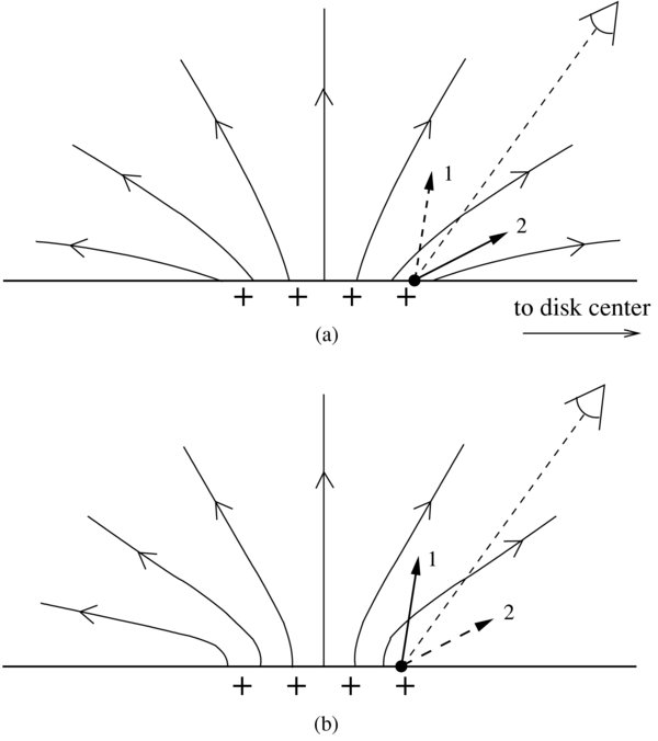
The observed magnetic vectors are subject to the usual 180° ambiguity in the azimuth angle of Bobs with respect to the LOS. To resolve this ambiguity, we first construct a reference field Bref(R☉, λ, ϕ), and then select the azimuth of Bobs such that the vectors Bobs and Bref make an acute angle when projected onto the image plane. In the present case, the THEMIS FOV is about 35° from the disk center, and we find that using a potential field as a reference produces artifacts in the ambiguity solution even when the magnetic field does not deviate strongly from a potential field. Specifically, discontinuities appear in the magnetic vectors on the disk-center side of magnetic elements where the direction of the magnetic field suddenly changes by about 70° (twice the heliocentric angle). The problem is illustrated in Figure 12(a), which shows a vertical cross section of a magnetic element modeled as a potential field. The black dot indicates a point on the disk-center side of the magnetic element (right-hand side of the figure), and the two arrows labeled "1" and "2" are the two possible solutions typically found by THEMIS for the magnetic vector at such a point. Note that these vectors lie on opposite sides of the LOS to the observer (dashed line), consistent with a 180° ambiguity. The comparison of these vectors with the potential field would cause solution "2" to be selected as the best solution, because the potential field at the observed point is more highly inclined with respect to the vertical than the LOS to the observer. In fact, as we move from the center of the magnetic element toward the disk center, there is a sudden jump from solution "1" to solution "2," which causes the discontinuities in the directions of the magnetic vectors.
Figure 12. Resolution of the 180°ambiguity by comparison of the observed vectors with a reference field: (a) potential-field reference model; (b) non-potential reference model taking into account the effects of magnetic buoyancy. The arrows labeled "1" and "2" show the two possible solutions for the magnetic field at a point on the disk-center side of the magnetic element. The dashed line shows the direction to the observer. Solution "2" is the best fit when the potential field is used as a reference, but solution "1" is selected for the more realistic, non-potential reference model.
Download figure:
Standard image High-resolution image
We believe that these jumps in the directions of the magnetic vectors are artifacts due to the tendency of the potential field to spread out horizontally over the solar surface away from magnetic elements. It is well known that plage elements actually consist of multiple flux tubes with a small filling factor and kilogauss field strength (de Wijn et al. 2009). Such flux tubes are highly buoyant, so their orientation cannot deviate too far from vertical. Therefore, we believe a more realistic model for a plage element is that shown in Figure 12(b), where the magnetic field in the photosphere is closer to vertical. The comparison of the observed vectors with such a non-potential reference field would cause solution "1" to be selected as the best-fit solution. Therefore, deviations from the force-free state in the photosphere must be taken into account when resolving the 180° ambiguity. Our approach here is to use a non-potential reference field that is everywhere more vertically oriented than the potential field. This is not a general solution, but is possible here because there are no sunspots in the THEMIS FOV.
The reference field is constructed as follows. First, the radial component of the reference field on the photosphere is computed as Br = B∥/cos θ, where B∥ is the unambiguous LOS components of the THEMIS data, and θ is the heliocentric angle. Then a potential-field extrapolation is obtained, and the field is evolved according to the MHD induction equation while an upward force is applied in the photosphere. The purpose of this force is to simulate the effects of magnetic buoyancy on photospheric magnetic elements (Metcalf et al. 2008; Bobra et al. 2008). The resulting reference field remains close to the potential field at larger heights in the corona, but it deviates significantly from the potential field in the photospheric layers where the comparison with Bobs is made. Specifically, at the edges of magnetic elements the reference field is more vertically oriented than the potential field.