


ABSTRACT
The rapid and irreversible decay of penumbrae related to X-class flares has been found in a number of studies. Since the optical penumbral flows are closely associated with the morphology of sunspot penumbra, we use state-of-the-art Hinode data to track penumbral flows in flaring active regions as well as shear flows close to the flaring neutral line. This paper concentrates on AR 10930 around the time of an X3.4 flare on 2006 December 13. We utilize the seeing-free solar optical telescope G-band data as a tracer to obtain the horizontal component of the penumbral and shear flows by local correlation tracking, and Stokes-V data to register positive and negative magnetic elements along the magnetic neutral line. We find that: (1) an obvious penumbral decay appears in this active region intimately associated with the X3.4 flare; (2) the mean magnitude of the horizontal speeds of the penumbral flows within the penumbral decay areas temporally and spatially varies from 0.6 to 1.1 km s−1; (3) the penumbral flow decreases before the flare eruption in two of the four penumbral decay areas; (4) the mean shear flows along the magnetic neutral line of this δ-sunspot started to decrease before the flare and continue to decrease for another hour after the flare. The magnitude of this flow apparently dropped from 0.6 to 0.3 km s−1. We propose that the decays of the penumbra and the penumbral flow are related to the magnetic rearrangement involved in the coronal mass ejection/flare events.
Export citation and abstract BibTeX RIS
1. INTRODUCTION
It has been well established that large-scale solar eruptions, e.g., solar flares and coronal mass ejections (CMEs), are magnetic in nature. Magnetic energy accumulating in the corona due to photospheric motions and flux emergence is released during the eruptions, and the coronal magnetic field becomes less nonpotential. As the lower boundary of the involved magnetic structure and the only layer where the magnetic field is routinely observed, the photosphere may also display some variations in magnetograms. Therefore, studies of the magnetic structure evolution in solar active regions are vitally important to the understanding of the physics of solar flares and CMEs. In recent years, several observations showed convincing evidence that rapid δ-spot penumbral decays are associated with X-class flares, and the neighboring umbral cores are simultaneously darkening as well (Wang et al. 2002a, 2002b, 2004; Liu et al. 2005; Deng et al. 2005), confirming the early discovery revealed by Howard (1963). Spirock et al. (2002) reported the evolution of magnetic field, a rearrangement of the magnetic field in a projected configuration, associated with a X20 flare. Sudol & Harvey (2005) and Li et al. (2008) confirmed that optical intensity changes are tightly related with photospheric magnetic field variations in X-class flares. Later, Chen et al. (2007) surveyed over 400 events and statistically concluded the trend that the darkening is more concentrated near the flaring neutral line in larger flares. Wang et al. (2004) proposed that magnetic fields in the penumbral decay areas partially change from more inclined to more vertical, accompanying the occurrence of solar flare. Yurchyshyn et al. (2004) proposed that the tether-cutting model (Moore & Labonte 1980; Sturrock 1989; Moore & Roumeliotis 1992) can explain the stretching of the outer field line and the formation of a new field line near the flaring neutral line. In particular, the tether-cutting could interpret the enhancement of transverse fields after flare. Deng et al. (2005), on the other hand, explained the phenomenon in terms of the field lines turning to more vertical positions in the breakout model framework. During an X-class flare, the rearrangement of magnetic field structures would also induce mass motions in the magnetized solar atmosphere, therefore variations of the plasma motions are expected.
Inside a sunspot group, the photosphere manifests two kinds of notable optical motions. One is the Evershed flow in the penumbra, and the other is the shear flow along the magnetic neutral line between positive and negative polarities. The Evershed effect, discovered by Evershed (1909), is height dependent, decreasing rapidly with the height (see e.g., Solanki 2003). Evershed flow carries magnetized gas (Solanki et al. 1992, 1994), and is restricted to the horizontal component of magnetic fields (Title et al. 1993; Degenhardt 1991). It was also found that Evershed flows begin to be visible when a penumbra forms (Leka & Skumanich 1998). This suggests that the Evershed flow pattern is coupled with the morphology of local magnetic fields. The speed of the Evershed flow should be measured spectrocopically (Shine et al. 1994; Tritschler et al. 2004; Sánchez Cuberes et al. 2005; Sánchez Almeida et al. 2007). However, the optical penumbral flow (which we assume is related to the Evershed flow) can be measured from imaging observations. The measurement of penumbral flow can provide information on Evershed flow. Naturally, one critical question is: is there a penumbral flow change associated with flares and the penumbral decay?
Shear flows, in photospheric and chromospheric layers, along the magnetic neutral lines can build up magnetic energy in flaring regions (Harvey & Harvey 1976; Amari et al. 2000; Yang et al. 2004). The moving plasma drags the magnetic field lines to form a nonpotential magnetic topology, so the shearing motions are a signature of the accumulation of magnetic nonpotentiality (Zhang 2001; Falconer 2001; Wang et al. 2006). The free magnetic energy will be released and the potential configuration will be restored after the sheared field reaches its critical point. Furthermore, shear motions could accumulate the magnetic helicity (Chae 2001) and form magnetic "channel" structures (Zirin & Wang 1993). Denker et al. (2007) concluded that the shear flows are commonly presented in complex sunspots but not related to the local magnetic shear. However, it is still not clear whether the shear flow can be affected by the energy releasing process during solar flare.
With the above two questions in mind, we investigate the changes of optical penumbral flows and shear flows associated with the X3.4 flare on 2006 December 13. In Section 2, the data set and the processing are described. The results are presented in Section 3, which is followed by some discussions in Section 4.
2. OBSERVATIONS AND DATA ANALYSIS
On 2006 December 13, which was close to the recent solar minimum, an X3.4-class two-ribbon flare erupted in the active region AR10930. The flare event, which was associated with a halo CME, was observed by various ground-based and space-borne telescopes, and has been studied extensively. The recently launched Hinode mission (Kosugi et al. 2007) provides unprecedented continuous high resolution observations of the solar atmosphere. The Solar Optical Telescope (SOT; Suematsu et al. 2008; Tsuneta et al. 2008) on board Hinode provides G-band (430.5 nm) images through the Broadband Filter Imager (BFI) and Stokes-V (Fe I 630.2 nm) observations from the Narrowband Filter Imager (NFI). In this paper, we concentrate on the variation of the flow motions in the source region, using the SOT G-band and Stokes-V data. The main data set is selected from 01:00:32 to 04:36:37 UT on 2006 December 13, covering the peak time of the X3.4 flare at 02:14 UT. In addition, the data from 20:44:36 on 2006 December 11 to 00:58:40 on 2006 December 12 are analyzed for comparison to a flare-free period. The pixel sizes are 0 109 (G band) and 016 (Stokes-V), or the nominal resolutions are about 0218 (G band) and 032 (Stokes-V). The cadence for both observations is 2 minutes. The field of view is about 100'' × 100''. The 2 minute cadence data offers a possibility to measure the plasma motions in the photosphere with the local correlation tracking (LCT) method (November & Simon 1988; Simon et al. 1988).
For the LCT calculations, the sequence of images was aligned and registered to remove drifts and occasional jumps from the Hinode tracking system. We then used a technique similar to that of Simon et al. (1988). It works by comparing bounded cells in each image with the same cells in the subsequent image. The rigid shift that gives the best match for each cell pair is interpreted as an (x, y) offset for the center of the cell. The shifted cells are apodized with a centered Gaussian. The cell centers are spaced 0109 apart for the G-band images. The FWHM of the two-dimensional (2D) Gaussian apodization is twice this and hence the resolution is also about twice the cell spacing. Even though seeing is not an issue with Hinode data, there is still noise in the LCT velocities resulting from random motions, oscillations, and perhaps photon noise. Hence, each cell is binned by around 4 by 4 grids. Also, a running temporal averaging was applied to reduce the noise in the individual LCT signals. The temporal window applied is 20 minutes, which includes 11 successive velocity maps. These are averaged and the ending time of each time window is assigned to the mean velocity field. Because portions of the areas contain motions other than the penumbral flows, we use a threshold of 0.2 km s−1 to eliminate low-amplitude motions and also reject any vectors that were not within 90° of the nominal outward direction. Only the selected vectors were taken into account for average velocity calculations. This makes the result a better measure of the optical penumbral flow.
Limb darkening is an effect of the solar atmospheric temperature gradient (Milne 1921). Correction of the limb darkening should be the very first step of this study. However, the G band is not a continuum window but heavily populated with lines. Motivated by Langhans & Schmidt' work (2002), we select a calibration line in a pure granulation area (see Figure 1), and fit the G-band intensity along the straight line with a fifth order polynomial in the variable μ, i.e., I' = c0 + c1μ + c2μ2 + c3μ3 + c4μ4 + c5μ5, where I' is the best fitted intensity along the calibration line, and μ = cos θ, θ is the angular central meridian distance. The coefficients resulting from the fitting are c0 = −3.60350 × 10⁶, c1 = 1.64239 × 10⁷, c2 = −2.73969 × 10⁷, c3 = 1.89836 × 10⁷, c4 = −3.35536 × 10⁶, and c5 = −1.05473 × 10⁶. Then, each pixel of the original G-band image is corrected by the following formula:

Here, Im is the measured intensity and 1500 is a biased constant to make I positive and closer to Im.
Figure 1. Correction of east–west limb darkening effect. The top panel is the Hinode SOT G-band image on 01:00:32 UT 2006 December 13. The calibration line (white solid line) indicates the position where the G-band (430.5 nm) intensity is fitted along. The calibration line contains only pixels with quiet Sun granulation. The dotted-dash box is the FOV focused in this study. Contours K1 and K2, derived from G-band difference image, indicate positions of flare kernels. Panel (a) is the original intensity along the calibration line versus μ (cosθ). The black solid line is the fifth order polynomial fitting. Panel (b) shows the corrected intensity and the best fitting.
Download figure:
Standard image High-resolution imageThe raw intensity images give us projected features in the plane of the sky because the active region is located around S05W33. The real pixel size and the derived velocities are subject to foreshortening. Therefore, we constructed the image in the heliographic plane and derotated the image sequence to the disk center to mainly justify the pixel size shrinkages in solar latitude and longitude (similar to Gary & Hagyard 1990; see Figure 2). Thus the projection effect is removed, and the LCT sampling window and Gaussian weighing function can be symmetric.

Figure 2. Comparison of original and projection corrected images. The left panel is the original (or projected) G-band image on 01:00:32 UT 2006 December 13. The right panel is the projection corrected (or deprojected) image.
Download figure:
Standard image High-resolution imageUsing the LCT method, the G-band images are processed to derive flow motions in the entire field of view (FOV). For the shear flow along the magnetic neutral line, the Stokes-V images are coregistered (or overlapped) in order to distinguish the positive and negative magnetic elements and then to separate their velocities. Here, we define the shear velocity as the difference between positive and negative polarity elements in the direction parallel to the complex of magnetic neutral line (Wang 2006), i.e.,

where  and
and  are the mean velocities of the positive and negative magnetic elements parallel to the magnetic neutral line, respectively. Both the velocities are projected in the direction of the neutral line. Note the shear velocity is the relative speed between positive and negative magnetic elements along the neutral line. A positive Vshear means that the shear flow (or relative velocity between positive and negative magnetic elements) direction is clockwise for this specific case.
In this study, the penumbral decay is quantitatively described by the difference intensity which can be calculated by the formula

where I(t) is the G-band intensity of each area at time t and t0 is the start time of the observation. The average velocity of the flow depends on the velocity vectors selected. The average difference intensity depends on the area selected.
3. RESULTS
The G-band images before the flare (at 01:00:32 UT) and after the flare (at 04:36:37 UT) are plotted in the left and middle panels of Figure 3, respectively. The difference image is shown in the right panel, where the significant enhancement of the difference intensity in the bright areas near the penumbra indicates that the penumbra locally decayed after the flare, and intensity dimming indicates that the penumbra is locally enhanced. It is seen that, contrary to the flare ribbons that appeared along the common penumbra between the upper and lower sunspots and flare kernels usually located in the strong magnetic fields (see kernels K1 and K2 in Figure 1), the penumbral decay is significant mainly on the outer side of the sunspot group, i.e., the north side of the upper sunspot and the south side of the lower sunspot, consistent with previous studies (e.g., Wang et al. 2004; Liu et al. 2005; Deng et al. 2005).

Figure 3. Left panel is the G-band image before the X3.4 flare on 01:00:32 UT 2006 December 13. The middle one is the image after the flare on 04:36:37 UT 2006 December 13. The right panel is the difference image (postflare image minus preflare G-band image). It was smoothed with a kernel of 20 × 20 pixels. The blue areas (A1, A2, A3, A4, N1, N2) are penumbral decay areas. The red region (D) is the penumbral enhanced area.
Download figure:
Standard image High-resolution imageThe difference image in Figure 3 is spatially smoothed by a kernel of 22. The bright areas, labeled A1, A2, A3, A4, N1, N2 and defined by blue contour lines, are penumbral decay areas, and the dark area (labeled D) defined by the red contour line represents the penumbral enhancement area. Area N1 is located in the common penumbra, while the difference intensity enhancement of area N2 is due to fast motion of a pore structure. We only take account of major enhanced areas (A1, A2, A3, A4) in this work.
The penumbra decay areas are outlined in Figure 4 by white curves. The boundaries of areas A3 and A4 are manually modified to avoid the pores. For comparison, we select a nondecay area, labeled A5. The horizontal flow field at 01:10:33 UT, which is derived from consecutive G-band images with the LCT method, is overplotted as vector arrows. It is seen that the flows in the selected areas are mainly radially outward along the penumbral fibrils, which is a typical feature of the penumbral flow in most penumbrae. However, in the common penumbra between the north and south sunspots, the photospheric motion significantly deviates from radial and is nearly tangential to the rotating sunspot to the south. Note that the measured granular LCT speed is mainly between 0.5 and 1 km s−1, which is comparable with previous results of 650 m s−1 (Wang et al. 1995) and 700 m s−1 (Berger et al. 1998).

Figure 4. G-band image flow map on 1:10:33 UT 2006 December 13. The areas (A1, A2, A3, A4) are penumbral decay areas corresponding to the markings in Figure 1. The area A5 is a reference area that the penumbra did not change much after the flare. The orange arrows indicate the magnitude and direction of flow velocity. The pink labels P1, P2, and P3 are the major pores.
Download figure:
Standard image High-resolution imageThe temporal evolutions of the mean values of the G-band intensity (diamonds) and the penumbral flow velocity (black asterisks) for the five selected areas are displayed in Figure 5. The flare peak time is indicated by a vertical dashed line in each panel. Figure 5(a) reveals that in the area A1, the penumbral intensity was almost constant before the flare and it started to increase near the flare peak time. One hour later, the G-band intensity increased to its maximum. Correspondingly, the penumbral flow in the same area showed a trend of decreasing from ∼0.96 to ∼0.85 km s−1 on average in the observation time window with visible oscillations. The evolutions of the G-band difference intensity and the penumbral flow in area A2 (Figure 5(b)) show a similar behavior, but with a systematic delay of ∼20 minutes. The magnitude of the penumbral flow decreased from ∼1 to 0.9 km s−1. The G-band difference intensity increases after the occurrence of the flare in both areas A3 and A4. However, the penumbral flow velocity stays almost invariant in area A3 about ∼0.6 km s−1, and varies from ∼0.70 to ∼0.77 km s−1 in area A4 across the flare peak. For comparison, we plot the evolution of the mean values of the G-band difference intensity (diamonds) and the penumbral flow velocity (black asterisks) of area A5 in Figure 5(e). It is seen that both quantities do not show significant variation across the flare peak, except that the penumbral flow velocity shows a slight trend of increasing oscillation amplitude.
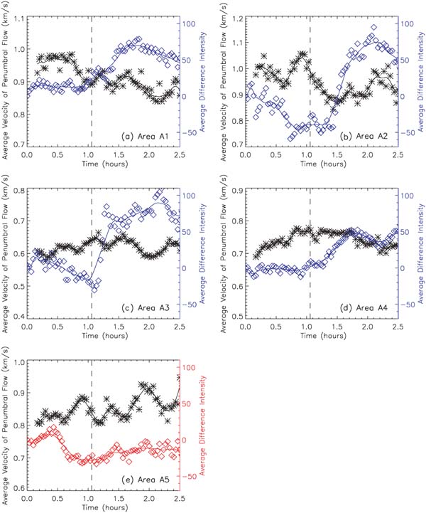
Figure 5. Time profiles of penumbral flows and G-band intensities. The black asterisks represent the magnitudes of the average velocity of horizontal penumbral flows in each area. The diamonds are the average difference intensities of each area. The solid curve shows the evolution tendency of each area. Figures 5(a)–5(e) correspond to the areas A1–A5 in Figure 2. The start time of plots is 1:10:33 UT 2006 December 13. The vertical dashed line indicates the flare time. The red color represents the intensity in the reference region.
Download figure:
Standard image High-resolution imageThe plasma motion in the common penumbra between the positive sunspot (the northern one) and the negative sunspot (the southern one) is driven by gradual rotation of the negative sunspot. This is manifested as a shear flow along the magnetic neutral line as shown mainly in the common penumbral area (see Figures 4 and 6). Figure 7 shows the evolution of the mean difference of the shearing velocity between the positive and negative magnetic elements in the region A6 that is enclosed by a white box in the right panel of Figure 6. The mean velocity difference decreased from ∼0.6 km s−1 30 minutes before the flare peak to ∼0.3 km s−1 30 minutes after the flare peak. The shear flow in the common penumbra is also oscillating, with a quasi-period of ∼50 minutes, which is almost identical to or slightly longer than those in the areas shown in Figure 5.

Figure 6. Left panel is the G-band intensity on 1:10:33 UT 2006 December 13. The middle one is the co-aligned corresponding Stokes-V data (Fe I 630.2 nm). The right panel is the G-band image contoured with Stokes-V image. The red contour represents positive polarity and the blue is negative. The boxed area A6 is the strong shear flow region.
Download figure:
Standard image High-resolution image
Figure 7. Evolution of shear flows covering the flaring period. The asterisks represent the average velocity of shear flows in the box area A6 in Figure 6. The start time of plot is 1:10:40 UT 2006 December 13. The vertical dashed line indicates the flare time.
Download figure:
Standard image High-resolution image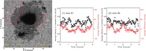
Figure 8. Left panel is the G-band image on 20:54:35 UT 2006 December 11. The red patches (B1, B2) are the reference penumbral areas. The middle and right panels are the evolutions of penumbral flows covering four-hour flare quiet time interval in areas B1 and B2. The start time of plots is 20:54:35 UT 2006 December 11.
Download figure:
Standard image High-resolution image4. DISCUSSION
Comparing the G-band images before and after X-class flares, Wang et al. (2004) and Deng et al. (2005) discovered penumbral decays associated with the eruptions. Such a feature was confirmed to be quite common in strong flare events (Liu et al. 2005). With the help of the optical observations by the newly launched Hinode satellite, we can study the timely evolution of the penumbral decay for the first time. In this paper, we analyzed the optical data for the X3.4-class flare on 2006 December 13. We find that while the two-ribbon flare appeared along the magnetic neutral line between the bipolar sunspots, the penumbral decay areas were basically located on the outer side of each sunspot, as indicated by Figure 3. In each segment of the penumbral decay areas, the G-band intensity was seen to increase for ∼50–70 DN after the flare peak, with a relative amplitude of ∼6% − 8%. It should be noted here that the penumbral decay studied in the earlier papers (e.g., Wang et al. 2004; Deng et al. 2005; Liu et al. 2005) was usually associated with umbral darkening, which is absent in our case as implied by Figure 3. However, the absence of umbral darkening is actually not rare. According to our recent statistical research, quite a lot of penumbral decay events did not show umbral darkening (Chen et al. 2007). The difference can be understood as follows. According to Wang et al. (2004) and Liu et al. (2005), the penumbral decay is attributed to the rearrangement of magnetic field from being more horizontal to more vertical during solar eruptions. While the penumbral magnetic field is significantly redirected, the transverse field will be enhanced near the magnetic neutral line, that would influence the umbral magnetic fields and lead to umbral darkening. However, if the common penumbral magnetic field horizontally changes its direction by a small angle during the solar eruption, it would not affect the umbra that much, as in our case.
As mentioned above, the penumbral decay was explained by Wang et al. (2004) to be produced when the more inclined magnetic field lines are stretched upward to become more vertical during the CME/flare eruptions, which was confirmed by recent vector magnetogram observations (Li et al. 2008). Since the outer penumbral flows tend to appear in areas with nearly horizontal magnetic field (Title et al. 1993), we expect to see a decrease of the outer penumbral flow associated with the magnetic field line stretching in the penumbral decay areas. During the quiescent stage, the penumbral flow was found to be oscillating with periods ranging from several up to 40 minutes (Shine et al. 1994; Rimmele 1994; Georgakilas & Christopoulou 2003; Cabrera Solana et al. 2007) which is consistent with our observation. Besides the intrinsic oscillation behavior, changes in fine structures might also be attributed to some residual jitters because of the limitations of LCT techniques (Simon et al. 1995). As indicated in Figure 5, among the four segments with penumbral decay, the areas A1 and A2 did show a significant decrease in the penumbral flow after the occurrence of the strong flare. The mean value of the optical penumbral flow velocity decreased by ∼0.1 km s−1 (about 10%) for both segments. However, the mean velocity of the penumbral flow in the areas A3 and A4 was almost constant across the flare event despite the penumbral decay. It is noted that a rotating pore (P3 in Figure 4) was located near the segment A4, and the other segment A3, as a part of the fast rotating positive sunspot, was in dynamic evolution. Therefore, the unexpected behavior of the penumbral flow in these two segments is probably due to the dynamic evolution in the surrounding photosphere. More surprisingly, the mean velocity of the penumbral flow in the area A5 (an area with relatively constant intensity) increased by ∼0.1 km s−1 across the flare occurrence.
The Evershed effect manifests itself in Doppler shifts and asymmetries of spectral lines. Therefore, it can be determined reliably only based on spectroscopic observations. However, we assume that there is a relationship between the optical penumbral flows and the Evershed flow. Fortunately, there are two observations from Hinode/SOT spectro-polarimeter (SP) near the X3.4 flare with 8 hr temporal interval. One is at 20:30 UT 2006 December 12 before the flare, the other is at 04:30 UT 2006 December 13 after the flare (see Figure 9). The bottom two images are the dopplergrams measured from the doppler shift at wavelength 6301.5 Å. Table 1 presents the variation of Evershed flows in selected areas which is consistent with the variation of optical penumbral flow. The optical penumbral flow and the Evershed flow both decreased about 10% in areas A1 and A2 after the major flare.

Figure 9. Images in the left column are at 20:30 UT 2006 December 12 (before the major flare). They are G-band, Hinode/SOT Stokes-V from NFI, Hinode/SOT spectro-polarimeter (SP) magnetogram and Hinode/SOT SP dopplergram, respectively from top to bottom. The images in the right column are at 04:30 UT 2006 December 13 (after the major flare). The areas (A1, A2, A3, A4, A5) are the areas corresponding to the markings in Figure 2.
Download figure:
Standard image High-resolution image
Table 1. Variation of Doppler Velocities in Selected Areas Before and After the Flare
| A1 | A2 | A3 | A4 | A5 | |
|---|---|---|---|---|---|
| Before (km s−1) | −4.23 a | −2.47 | −3.76 | −3.16 | −2.92 |
| After (km s−1) | −3.80 | −2.17 | −3.76 | −3.16 | −2.86 |
| Decrease | 10.2% | 12.1% | ... | ... | 2.1% |
Notes. aThese values are area-averaged. The negative sign means the direction is from the sun toward the observer. Poor fitting points are removed.
Download table as: ASCIITypeset image
In order to further confirm that the variations of the penumbral flow and the penumbral intensity were associated with the CME/flare eruption, we investigate the temporal evolution of the same sunspot group one day before the CME/flare eruption, when it was flare-free. Two patches of the penumbra are selected and labeled "B" and "B" in the left panel of Figure 8. The evolution of the G-band difference intensity (diamonds) and the penumbral flow velocity (asterisks) for the two patches are displayed in the middle and right panels. Note that the average value of the G-band intensity in the 4 hr data set is subtracted from the observed intensity to obtain the difference intensity. We see that both the difference intensity and the penumbral flow velocity were oscillating, with amplitudes of ∼±40 DN and ∼±0.09 km s−1, respectively. However, both quantities did not show any trend of increasing or decreasing during 4 hr. This reinforces the idea that the penumbral decay and the penumbral flow decrease in segments A1 and A2 are intimately associated with the CME/flare eruption, or more precisely, they are caused by the stretching of the magnetic field lines associated with the CME/flare eruption.
Shear flows are often present along the magnetic neutral line, which is responsible for the energy built-up in active regions (e.g., Wang 1992). In the event analyzed in this paper, the magnetic neutral line happened to be along the common penumbra of the sunspot group. Therefore, shear flow also showed some features present in the penumbral flow, e.g., the quasi-periodic oscillation of the flow velocity as indicated by Figure 7. The striking feature shown in this figure is that the shear flow velocity dropped down rapidly from ∼0.6 km s−1 to ∼0.3 km s−1 in association with the CME/flare eruption. This can be understood as follows. Before the CME/flare event, magnetic shear was increasing continuously due to the rotation of the southern sunspot (Zhang et al. 2007). As the nonpotentiality increases, the magnetic system in the corona approached a critical point, after which it became unstable. The stored magnetic energy was then released to be manifested as the CME and flare, during which the magnetic field lines were untwisted. As a result, the shear flow speed decreased. In other words, the decrease of the shear flow speed across the magnetic neutral line could be regarded as a signature of the magnetic energy relaxation. It should be noted that the shear flow slowed down, but did not stop. It kept moving in the original direction even after the CME/flare eruption. Probably it is such a continual shear flow along the magnetic neutral line that led to the increase of the magnetic shear in the photosphere after the flare, compared to the pre-eruption stage 8 hr earlier, as found by Jing et al. (2008). It was, however, noted by (Denker et al. 2007) that the photospheric shear flow along the magnetic neutral line was not related to any change of the local magnetic shear in their case. They emphasized the important role of the global magnetic twist of the δ spot field.
In summary, for the first time, we tracked the evolution of the penumbral decay process associated with a CME/flare eruption with 2 minute cadence from space, and found that the eruption was also accompanied by a decrease of the optical penumbral flow and the Evershed flow in the penumbral decay areas. Both features are probably the direct signature of the magnetic field stretching in the CME eruption. It is also found that the shear flow across the magnetic neutral line decreased in response to the magnetic energy release.
The authors thank Dr. Richard A. Shine for providing the LCT codes, reading the manuscript and valuable comments. The authors also thank Dr. Carsten Denker for discussion and the referee for constructive suggestions. Hinode is a Japanese mission developed and launched by ISAS/JAXA, collaborating with NAOJ as a domestic partner, NASA and STFC (UK) as international partners. Scientific operation of the Hinode mission is conducted by the Hinode science team organized at ISAS/JAXA. This work is supported by NASA under grant NNXO-7AH78G and NSF under grant ATM-0716512.