


ABSTRACT
It is well known that a complete description of the solar wind requires a kinetic description and that, particularly at sub-proton scales, kinetic effects cannot be ignored. It is nevertheless usually assumed that at scales significantly larger than the proton gyroscale rL, magnetohydrodynamics or its extensions, such as Hall-MHD and two-fluid models with isotropic pressures, provide a satisfactory description of the solar wind. Here we calculate the polarization and magnetic compressibility of oblique kinetic Alfvén waves and show that, compared with linear kinetic theory, the isotropic two-fluid description is very compressible, with the largest discrepancy occurring at scales larger than the proton gyroscale. In contrast, introducing anisotropic pressure fluctuations with the usual double-adiabatic (or CGL) equations of state yields compressibility values which are unrealistically low. We also show that both of these classes of fluid models incorrectly describe the electric field polarization. To incorporate linear kinetic effects, we use two versions of the Landau fluid model that include linear Landau damping and finite Larmor radius (FLR) corrections. We show that Landau damping is crucial for correct modeling of magnetic compressibility, and that the anisotropy of pressure fluctuations should not be introduced without taking into account the Landau damping through appropriate heat flux equations. We also show that FLR corrections to all the retained fluid moments appear to be necessary to yield the correct polarization. We conclude that kinetic effects cannot be ignored even for krL ≪ 1.
Export citation and abstract BibTeX RIS
1. INTRODUCTION
Magnetohydrodynamics (MHD) has been used for many years to describe solar wind turbulence theoretically and to interpret observational data (see reviews by Goldstein et al. 1995; Tu & Marsch 1995; Bruno & Carbone 2005; Horbury et al. 2005). It is generally accepted that at scales large compared with the proton gyroscale (i.e., krL ≪ 1) in the inertial range of the turbulence spectrum, MHD provides a satisfactory description of the physical properties of the (almost) collisionless solar wind.
Recent observational studies have spanned spatial scales smaller than the proton gyroscale, and in some cases even down to electron scales (see, e.g., Alexandrova et al. 2009; Sahraoui et al. 2009, 2010; Perri et al. 2012). Some of these studies support the idea that at sub-proton scales the turbulent cascade is dominated by nonlinearly interacting kinetic Alfvén waves (KAWs; Bale et al. 2005; Sahraoui et al. 2009, 2010; Salem et al. 2012). Other studies maintain that the most relevant mode is the whistler wave (see, e.g., Gary & Smith 2009; Podesta et al. 2010; Gary et al. 2012) or that none of the modes alone can explain the observations (Narita et al. 2011; Smith et al. 2012). A correct understanding of the physical properties of KAWs is critically important and, as was shown recently by Sahraoui et al. (2012), these properties still need to be explored. Furthermore, any fluid model that purports to describe the large-scale solar wind should capture the correct linear properties of KAWs. A main issue addressed in this paper concerns the need of retaining low-frequency kinetic effects within a fluid description, even at large scales.
Even though extensions of MHD such as Hall-MHD and two-fluid models provide additional physics by including the Hall-term and introducing anisotropic pressure fluctuations for protons and electrons, one of the biggest deficiencies is the unphysical description of damping in the collisionless regime. By and large, fluid models either mimic the Navier–Stokes approach of employing Laplacians to control damping (or use hyperresistivity and hyperviscosity) or rely on sophisticated numerical schemes to avoid the development of unphysical gradients or numerical instabilities. To address this issue, a new class of the so-called Landau fluid models has been developed that incorporate kinetic effects, such as linear Landau damping. In that way, collisionless wave damping is introduced into the fluid description. The simplest Landau fluid closures are parallel propagating slab models (Hammett & Perkins 1990). The associated equations were numerically explored by Jayanti et al. (1998) in an investigation of the parametric decay of Alfvén waves.
The first Landau fluid model to account for different parallel and perpendicular pressures and heat fluxes and, therefore, to incorporate linear Landau damping (by both protons and electrons) into a fully three-dimensional (3D) geometry was presented by Snyder et al. (1997). This model was derived from the drift kinetic equation. By construction, this approach neglects the Hall-term and non-gyrotropic contributions such as finite Larmor radius (FLR) corrections because the drift kinetic ordering sets the proton gyroradius, rL, to zero. We refer to it as the large-scale(LS)-Landau fluid where, in the following, we retain the Hall effect as it introduces dispersive effects. A LS-Landau fluid model of Snyder et al. (1997) was used by Chandran et al. (2011) to develop a 1D turbulence transport solar wind model.
Over the last decade, the Landau fluid approach was reconsidered and refined to its present form by Passot & Sulem (2003, 2004), Goswami et al. (2005), Passot & Sulem (2006, 2007), and Passot et al. (2012). Their approach begins directly from the Vlasov equation and is therefore able to incorporate kinetic effects including a non-zero Larmor radius. In these Landau fluid models, FLR corrections to all the retained fluid moments can be evaluated in two different ways. One choice is to employ a scale separation expansion of the pressure and heat flux tensor equations in both space and time. The alternative approach is to evaluate the FLR contributions directly from linear kinetic theory in the low-frequency limit (Passot & Sulem 2007; Passot et al. 2012). To prevent confusion between models with different FLR corrections, Passot et al. (2012) suggested that the former class of models be referred to as meso-scale (MS) Landau fluids and the latter class as FLR-Landau fluids.
We will adopt those definitions in this paper (we note that the model used by Hunana et al. 2011 for the first 3D Landau-fluid simulations of turbulence should have been called MS-Landau fluid instead of FLR-Landau fluid). Here we use the FLR-Landau fluid model and the LS-Landau fluid model to explore the importance of kinetic effects in understanding KAWs (for simplicity, the MS-Landau fluid model is not considered here). The exact equations of the LS-Landau fluid model are written down in Appendix A, where the FLR-Landau fluid model is also briefly described by referring to equations of Passot et al. (2012).
In the isotropic two-fluid model that does not contain any kinetic effects, but still contains the Hall-term, the (isotropic) proton and electron pressures are prescribed as  . Here we adopt the usual values of the proton polytropic index γp = 5/3 and the electron index γe = 1. To introduce the anisotropy of pressure fluctuations, we use the usual CGL equation of state (Chew et al. 1956) for both particle species and we call this model "CGL protons + CGL electrons." We also briefly consider model where the protons obey the CGL condition and the electrons are isotropic, we call this model "CGL protons + Iso electrons." All these usual fluid models are derived with the assumption of vanishing heat fluxes. Differently, the Landau fluid models involve dynamical equations for the gyrotropic heat fluxes of the ions and electrons. Both Landau fluid models used here are closed at the level of the fourth-rank fluid moments (evaluated in a quasi-static approximation) and contain both proton and electron Landau damping. Electron inertia is neglected in all the fluid models since we concentrate on frequencies that are much smaller than the electron cyclotron frequency. The initial mean parallel and perpendicular pressures are taken equal, i.e., there is no mean temperature anisotropy present for both particle species. The mean electron temperature is taken equal to the mean proton temperature. Kinetic solutions require knowing the ratio of the proton thermal speed vth to the speed of light c, which we take to be vth/c = 10−4.
For each fluid model, the equations were linearized and the dispersion relation ω(k) calculated numerically for a given set of plasma parameters. Both Landau fluid models considered here consist of 15 dynamical equations in 15 variables and, together with the divergence free constraint for the magnetic field, yield 14 different waves. Some of these solutions are very highly damped and are not analogous to the usual MHD waves. This is consistent with kinetic theory, which yields an infinite number of highly damped solutions. For each wavenumber, the frequency is substituted back into the equations to (numerically) obtain the eigenvector. We used the WHAMP code (Rönnmark 1982) to find the solutions of the full linear kinetic theory. Comparison of mode properties in a two-fluid models and kinetic theory was also performed by Krauss-Varban et al. (1994) and Howes (2009).
2. NUMERICAL RESULTS
We first briefly explore how KAW polarization changes with θ (defined as angle between wavevector k and mean magnetic field  ), focusing on the large scales (krL < 1). It is known that for sufficiently large θ, the oblique KAW is right-hand polarized (see, Gary 1986; Belmont & Rezeau 1987; Hollweg 1999; Sahraoui et al. 2012). Figure 1 illustrates the angular transition of KAW polarization from left-hand to right-hand polarized wave as the proton plasma beta increases from β = 0.01 (Figure 1, left) to β = 0.1 (Figure 1, center) to β = 2.0 (Figure 1, right). Kinetic solutions are represented by solid lines and solutions of the FLR-Landau fluid model are represented by crosses. The polarization is defined as
  (left hand/right hand are negative/positive, respectively). In general, |Ex| ≠ |Ey|, so polarization
  does not necessarily imply that the wave is circularly polarized. For β = 0.01 (Figure 1, left) the KAW propagating at θ = 82° is a left-hand polarized wave with
  , while at θ = 85° the KAW is right-hand polarized with
  . The KAW completely changes polarization from −0.5 to +0.5 over a span of only 3°. For β = 0.1 (Figure 1, center), the complete change of polarization occurs between θ = 70° and θ = 75°. Finally, for β = 2.0 (Figure 1, right), the only left-hand polarized KAW with
  is the wave propagating at θ = 0° (red line). Then, as θ increases, the KAW smoothly changes its polarization from negative to positive values and becomes right-hand polarized. In this case, we also searched for an approximate value of θ for which the KAW is linearly polarized (
 ) and found that this occurs at θ = 42
 5 (magenta line). Therefore, it is worth emphasizing that for typical (high) values of plasma beta in the solar wind (β ⩾ 1), the KAW does not have to be highly oblique to be right-hand polarized. Solutions of the FLR-Landau fluid model are plotted only for three angles of propagation θ = 35° (blue crosses, left-hand polarized KAW), θ = 425 (magenta crosses, linearly polarized KAW), and θ = 45° (cyan crosses, right-hand polarized KAW). In all three β cases, the FLR-Landau fluid model accurately captures the angular transition of the KAW polarization at large scales. It is interesting to note that, while for lower beta the angular polarization transition occurs over only a few degrees, for higher beta this transition occurs over a much larger range in θ.

Figure 1. Polarization of KAWs with respect to length scale. Solid lines are kinetic solutions, and crosses are solutions of the FLR-Landau fluid model. Left: β = 0.01, θ = 82° (red) and 85° (blue). Center: β = 0.1, θ = 70° (red) and 75° (blue). Right: β = 2.0, θ = 0° (red), 25° (green), 35° (blue), 425 (magenta), 45° (cyan), 50° (black), and 89° (yellow).
Download figure:
Standard image High-resolution imageRecent studies of the evolution of magnetofluid turbulence in the solar wind have emphasized the importance of understanding the physical properties of highly oblique KAWs (k⊥ ≫ k∥), i.e., fluctuations with 80° ⩽ θ < 90°. This range of parameters was recently examined using the WHAMP code by Sahraoui et al. (2012) who showed that for KAWs to reach the electron scale and be sufficiently undamped, the (linear) wave had to propagate at extremely large values of θ, e.g., as much as 8999. This value of θ was used by Sahraoui et al. (2009) to interpret the power spectrum of magnetic fluctuations at very small spatial scales (of the order of and less than the electron Larmor scale).
The gyrokinetic description (Howes et al. 2006, 2008; Schekochihin et al. 2009) is also derived in the limit k⊥ ≫ k∥. At these extreme angles and spatial scales of order the electron Larmor radius, the only relevant wave particle resonance is electron Landau damping and even that interaction requires very fast particles from the strahl component of the solar wind electron distribution. Another implication of such large values of θ is the challenge of knowing the background magnetic field with sufficient precision so that θ can be accurately defined. In the discussion here we will use such extreme angles to explore kinetic effects in comparison to fluid predictions and will defer any discussion of their observational reality to another study. The angle θ = 8999 was also chosen for convenience to be able to plot all β parameters up to the same wavenumber k⊥rL = 10.
In Figure 2, we compare magnetic compressibility calculated from the four fluid models (crosses) and kinetic theory (solid lines) over scales ranging from k⊥rL = 0.01 to k⊥rL = 10. The proton plasma beta is taken to be β = 0.1 (red), 0.5 (green), 1.0 (blue), 2.0 (magenta), 4.0 (cyan), and 10.0 (black). The magnetic compressibility, χ, is defined as χ(k⊥rL) = |Bz(k⊥rL)|2/|B(k⊥rL)|2, where Bz(k⊥rL) is the parallel component of the total magnetic field B (in Fourier space). The compressibility predicted by the isotropic two-fluid model (Figure 2, top left) is very large when compared to the kinetic calculation and the discrepancy increases with β. The only exception comes at small β (cf., β = 0.1 in Figure 2). The discrepancy is most visible in the range k⊥rL = [0.1, 1] (note that in Figure 2 the y-axis is plotted using a linear scale). In Figure 3, the y-axis is plotted on a log scale and the large overestimate of χ is evident even for k⊥rL = [0.01, 0.1].

Figure 2. Magnetic compressibility χ(k⊥rL) of highly oblique KAWs with propagation angle θ = 8999 for the isotropic two-fluid model (top left), CGL protons + CGL electrons model (top right), large-scale Landau fluid model (bottom left), and FLR-Landau fluid model (bottom right). Solid lines represent kinetic theory and crosses represent solutions of the corresponding fluid models. The proton plasma beta is 0.1 (red), 0.5 (green), 1.0 (blue), 2.0 (magenta), 4.0 (cyan), and 10.0 (black).
Download figure:
Standard image High-resolution image
Figure 3. Similar to Figure 2 but with a logarithmic scale for compressibility χ, which emphasizes the large scales. The models are directly compared side by side, separately for each plasma β. The models are kinetic theory (red line), isotropic two-fluid (red crosses), CGL protons + Iso electrons (green crosses), CGL protons + CGL electrons (cyan crosses), LS-Landau fluid (blue crosses), and FLR-Landau fluid (black crosses). The proton plasma beta is 0.1 (top left), 0.5 (top right), 1.0 (center left), 2.0 (center right), 4.0 (bottom left), and 10.0 (bottom right).
Download figure:
Standard image High-resolution imageThe top right panel of Figure 2 compares the compressibility of the CGL protons + CGL electrons model with kinetic theory. It is shown that anisotropy of pressure fluctuations unrealistically reduces compressibility χ for all values of β. The exceptions are solutions for β = {0.5, 1.0} at very small scales, where the χ is enhanced. An interesting observation is that at small scales for β ⩾ 0.5, the compressibility decreases with β. This is in strong contrast with both the isotropic two-fluid and kinetic theory, where at small scales the compressibility increases with β.
The bottom left panel of Figure 2 compares the compressibility from the LS-Landau fluid model with kinetic theory. Landau damping corrects the large errors in compressibility χ introduced by the anisotropy of pressure fluctuations and the solutions for β ⩽ 2 are somewhat precise, even though slightly overestimated. However, the match with kinetic theory is not perfect and compressibility computed from this model for β = 4 and β = 10 is underestimated. Figure 2 (bottom right) compares the compressibility of FLR-Landau fluid model with the kinetic theory. The match with kinetic theory is quite precise on all scales and for all values of β. Evidently, FLR contributions are required in fluid models to reproduce accurately the compressibility χ of KAWs as computed from kinetic theory.
To further explore the compressibility at large scales, in Figure 3 we plot the χ in a logarithmic scale. The solutions are rearranged and all the models are compared side by side, separately for each plasma β. One new model is considered and that is the CGL protons + Iso electrons model. It is shown that for low β = 0.1, all the fluid models behave essentially in the same way and the compressibility χ is described quite accurately. The following generalizations therefore only concern the solutions with β ⩾ 0.5. The isotropic two-fluid is very compressible in comparison to kinetic theory for all values of β and for β ⩾ 1 it is the most compressible model, surpassed only for β = 0.5 by the CGL protons + Iso electrons model. The discrepancy between the isotropic two-fluid and the kinetic theory increases with β and for β = 10 the isotropic two-fluid overestimates the compressibility χ at large scales by two orders of magnitude. Considering only large scales k⊥rL < 1, the CGL protons + CGL electrons model is the model with the lowest amount of compressibility from all the fluid models and the compressibility is very far from the results of kinetic theory. For example, for β = 0.5 at scales around k⊥rL = 0.6, the compressibility is underestimated by well over four orders in magnitude. In contrast, the LS-Landau fluid model yields quite good values of compressibility χ for all range of β and all range of scales. The results demonstrate that the anisotropy of pressure fluctuations should not be introduced without an appropriate form of Landau damping. The compressibility χ for the FLR-Landau fluid model is extremely well reproduced for all ranges of scales and β. The results for CGL protons + Iso electrons are not conclusive and while for β ⩾ 1 the χ is reproduced quite accurately at large scales, at small scales for β = {1.0, 2.0} the compressibility χ is very off and for β = 0.5 it is the most compressible model at large scales.
The polarization is also sensitive to the approximations used. In the top-left panel of Figure 4, we compare  calculated from the isotropic two-fluid model and kinetic theory. The polarization
  is obtained for all β when calculated from the isotropic two-fluid model (note that the solutions are plotted over each other and only the last plotted solution with β = 10 is visible). The isotropic two-fluid model correctly describes highly oblique KAW as being right-hand polarized waves. However, the model completely misses the sensitive dependence of
  on β and also does not describe the dependence of
  on k⊥rL.

Figure 4. Polarization  of highly oblique KAWs. As in Figure 2, solid lines represent kinetic theory and the proton plasma beta is 0.1 (red), 0.5 (green), 1.0 (blue), 2.0 (magenta), 4.0 (cyan), and 10.0 (black).
Download figure:
Standard image High-resolution imageAnisotropic pressure fluctuations in the CGL protons + CGL electrons model (Figure 4, top right) do not introduce almost any variation in  and all considered solutions with β = {0.1, 1.0, 2.0, 4.0, 10.0} are right-hand polarized waves with
  . However, for β = 0.5 this model yields a KAW wave which is left-hand polarized at large scales with
  and only at smaller scales the KAW becomes right-hand polarized with
  .
.
Landau damping in the LS-Landau fluid model (Figure 4, bottom left) introduces some variation in  with β and k⊥rL, but, even though all the solutions are right-hand polarized waves, the solutions do not match the kinetic calculations. The only solution that is reproduced accurately is for low β = 0.1.
In contrast, the FLR-Landau fluid model (Figure 4, bottom right) correctly captures polarization for all values of β and all spatial scales. Obviously, the FLR corrections and non-gyrotropic corrections to the fourth-rank cumulants are crucial for a correct reproduction of KAW polarization. In fact, it is not surprising that the FLR-Landau fluid model correctly reproduces the linear kinetic theory in quasi-transverse directions, as the only approximation at the linear level is the replacement of the plasma response function by a Padé approximant. Note that the discrepancy between the two-fluid and FLR-Landau fluid models is still very evident at scales larger than the proton gyroscale. This is unexpected because it is usually assumed that FLR corrections become important only at sub-proton scales (k⊥rL > 1). Here we find that FLR corrections cannot be ignored, even at scales that are as large as k⊥rL = 0.01.
Figure 5 compares the real frequency ωr of these four different fluid models with kinetic theory. The frequency is normalized with respect to the proton cyclotron frequency Ωp. It is shown that the isotropic two-fluid (Figure 5, top left) describes the real frequency quite accurately for all range of scales and all range of β. In contrast, the CGL protons + CGL electrons model (Figure 5, top right) is very inaccurate in modeling the frequency at sub-proton scales k⊥rL > 1 for β = {0.5, 1.0, 2.0, 4.0}. Again, the introduction of Landau damping corrects the deficiencies introduced by the anisotropic pressure fluctuations and the solutions for the LS-Landau fluid model (Figure 5, bottom left) are quite precise. The solutions for the FLR-Landau fluid model (Figure 5, bottom right) are very precise.

Figure 5. Real frequency of highly oblique KAWs; all parameters are the same as in Figure 2.
Download figure:
Standard image High-resolution imageTo further verify these results, we calculated the KAW polarization and compressibility for the propagation angle θ = 60° at even larger scales (k⊥rL = [10−3, 10−1]) as shown in Figures 6 and 7. The colors are identical to those in Figure 2. All conclusions that hold for θ = 8999 are also valid for moderately oblique KAW propagation (θ = 60°).

Figure 6. Similar to Figure 2 but at 60° and with a logarithmic scale for χ. Proton β is 0.5 (green), 1.0 (blue), 2.0 (magenta), 4.0 (cyan), and 10.0 (black).
Download figure:
Standard image High-resolution image
Figure 7. KAW polarization  at θ = 60°. Proton β is 0.5 (green), 1.0 (blue), 2.0 (magenta), 4.0 (cyan), and 10.0 (black).
Download figure:
Standard image High-resolution imageFigure 6 (top left) shows that the isotropic two-fluid model is unrealistically compressible in the inertial range k⊥rL ≪ 1. The logarithmic scale reveals that for high values of β, compressibility can be overestimated by as much as two orders of magnitude when compared with kinetic theory. Figure 6 (top right) shows that incorporating anisotropic pressure fluctuations significantly reduces compressibility at very large scales. However, the system behaves quite strangely and while for β = 0.5 the compressibility χ is overestimated, in fact, already at β = 1.0, χ is very underestimated. Solutions for the LS-Landau fluid model are shown in Figure 6 (bottom left). Even though the compressibility is not captured completely accurately, the addition of Landau damping brings the fluid solutions much closer to kinetic theory. Finally, the FLR-Landau fluid (Figure 6, bottom right) does describe the compressibility χ with excellent accuracy.
The polarization  for KAWs propagating at θ = 60° is shown in Figure 7. The isotropic two-fluid model does not correctly describe polarization
  (Figure 7, top left) and examples with β ⩾ 0.5 have
  regardless of plasma β. The anisotropic pressure fluctuations in the CGL protons + CGL electrons model (Figure 7, top right) do not introduce any changes for β ⩾ 1 and all examples have
  . However, the solution with β = 0.5 has
  for all ranges of considered scales and the solution is very inaccurate. Landau damping in the LS-Landau fluid model (Figure 7, bottom left) partially cures this problem and the solution with β = 0.5 has
  and is quite accurate (the solution is overdrawn by the solution with β = 1.0 which has the same
  value). Landau damping alone however is inadequate to remove the large discrepancies in
  and the solutions deviate significantly from the kinetic calculations. Finally, the FLR-Landau fluid model (Figure 7, bottom right) does describe
  of KAWs with good accuracy.
The effect of Landau damping is perhaps most easily demonstrated by calculating the dispersion relations and plotting the damping rate (which is zero in the usual two-fluid models). The damping rates of KAWs for θ = 8999 are shown in Figure 8 and for θ = 60° in Figure 9. Figure 8 (left) shows that while for β = 0.1 the LS-Landau fluid model describes the damping rate quite accurately, for β = 0.5 the damping rate is underestimated at large scales and for β = 10.0 the damping rate is overestimated at large scales. The same observation holds for θ = 60° (Figure 9, left), where for β = 0.5 the damping rate is underestimated and for β = 10.0 the damping rate is overestimated. In contrast, it is shown (Figures 8 and 9, right) that the FLR-Landau fluid model accurately describes damping of KAWs for the range of θ, β, and spatial scales discussed in this paper. The damping rate increases with wavenumber so that KAWs become increasingly damped at smaller scales. Consequently, the effects of Landau damping become increasingly important at sub-proton scales (k⊥rL > 1), which is to be expected.

Figure 8. Damping rates of highly oblique KAWs (θ = 8999) for large-scale Landau fluid (left) and FLR-Landau fluid (right). Kinetic solutions are solid lines, and fluid solutions are crosses. Proton β is 0.1 (red), 0.5 (green), 4.0 (cyan), and 10.0 (black).
Download figure:
Standard image High-resolution image
Figure 9. Similar to Figure 8 but at θ = 60°. Proton β is 0.5 (green), 2.0 (magenta), and 10.0 (black).
Download figure:
Standard image High-resolution imageAt this stage it is important to mention that for typical solar wind parameters, electron Landau damping counts as a significant part of the global damping of KAWs even at scales comparable to the proton gyroradius. To demonstrate this, we used the FLR-Landau fluid model and prescribed the electrons to be isothermal (isotropic with γe = 1), which eliminates the electron Landau damping and only the proton Landau damping is present. We call this model "FLR-Landau fluid + isothermal electrons." Real and imaginary frequencies calculated from this model for highly oblique KAWs with θ = 8999 are shown in Figure 10. It is shown that the real frequencies (Figure 10, left) are not influenced by the lack of electron Landau damping and the solutions reproduce kinetic results with a very good accuracy for all ranges of scales and values of β considered here. The damping rate (Figure 10, right) is also reproduced very accurately at scales larger than the proton gyroscale k⊥rL < 1 for all solutions with β ⩾ 0.5. However, at scales comparable to the proton gyroscale k⊥rL ∼ 1, the damping rate is noticeably reduced and the reduction is further emphasized at sub-proton scales k⊥rl > 1. The special case is the solution for low β = 0.1, for which the damping rate is underestimated at large scales and somewhere between k⊥rL = 2 and k⊥rL = 4 the damping rate is actually positive (the KAW becomes unstable and the damping rate is out of the range in the logarithmic graph). These results demonstrate that the electron Landau damping is important already at scales comparable to the proton gyroscale, a fact that might impact the use of hybrid models with isothermal electrons at these scales.

Figure 10. Real frequency ωr/Ωp (left) and imaginary frequency −ωi/Ωp (right) for highly oblique KAWs (θ = 8999) calculated from FLR-Landau fluid model with isothermal electrons. The figure demonstrates the importance of electron Landau damping for ωi even at scales comparable to the proton gyroscale k⊥rL ∼ 1. Colors for proton β are the same as in Figure 2.
Download figure:
Standard image High-resolution image3. DISCUSSION AND CONCLUSIONS
The effect of Landau damping in fully nonlinear 3D simulation of turbulence was explored by Hunana et al. (2011), who compared simulations of a simple MS-Landau fluid model to simulations of the usual Hall-MHD model. They showed that Landau damping was responsible for strong damping of slow magnetosonic modes, which is consistent with the kinetic theory, and also that the power spectra of the magnetic and velocity fields with respect to k|| are much steeper in MS-Landau fluid simulations than in the usual Hall-MHD model. The scale-dependent magnetic compressibility, as defined here, was not directly calculated by Hunana et al. (2011). Instead, the velocity field was expressed as a solenoidal (incompressible) and non-solenoidal (compressible) decomposition and the associated energies were calculated by summing over all spatial scales in the simulation domain. Compressibility, defined as the ratio of the compressible energy to the total energy in the velocity field for the full solution (which, in addition to KAWs, contained all other possible modes and fluctuations), was shown to be significantly reduced in the MS-Landau fluid simulation.
The reduction of compressibility is important in the solar wind context as, even though the solar wind is a fully compressible medium, the turbulent fluctuations behave essentially as if they were incompressible. For a compressible MHD flow to display such a behavior, turbulent fluctuations must have initially very specific scalings with respect to the turbulent Mach number, as is known from the theory of nearly incompressible MHD (Zank & Matthaeus 1993; Hunana & Zank 2010; Bhattacharjee et al. 1999, and references therein) and from compressible hydrodynamic simulations (Ghosh & Matthaeus 1992; Passot & Pouquet 1987). However, there is no a priori reason why such specific initial conditions should be present in the solar wind. The addition of kinetic Landau damping to a fluid model strongly damps the slow magnetosonic modes and naturally reduces the compressibility of the flow regardless of the form of the initial conditions.
In the analysis presented here, the effect of Landau damping was demonstrated by calculating the KAW eigenvector and by evaluating the magnetic compressibility χ. We showed that the isotropic two-fluid model is very compressible in comparison with kinetic theory and, surprisingly, the largest discrepancy is at large scales (k⊥rL < 1). We showed that the anisotropy of pressure fluctuations introduced by the CGL protons + CGL electrons model drastically reduces the compressibility of KAWs at large scales. However, the anisotropy of pressure fluctuations leads to compressibility values which are very far from kinetic calculations. Very large errors in this model occur also for the real frequency ωr, especially at sub-proton scales and intermediate values of β. This is in contrast with the isotropic two-fluid for which the real frequency is reproduced quite accurately for all range of scales and values of β considered here. The addition of Landau damping appears to cure these problems and the LS-Landau fluid model indeed yields solutions which have compressibilities and real frequencies much closer to kinetic theory. From Figures 3 and 6, where the compressibility χ is plotted in a logarithmic scale, it is clearly visible that Landau damping strongly influences the compressibility even at the largest considered scales, i.e., k⊥rL = 0.01 and k⊥rL = 0.001. We conclude that the anisotropy of pressure fluctuations should not be introduced without retaining an appropriate form of Landau damping, even at scales much larger than the proton gyroscale.
An interesting result also concerns the polarization of the electric field  , for which we have shown that the isotropic two-fluid model yields very incorrect values at scales as large as k⊥rL = 0.001 and possibly larger. From the models considered here, only the FLR-Landau fluid model was able to correctly capture the polarization. To better understand this result, in Appendix B we consider two additional fluid models, where FLR corrections are supplemented to the usual fluid models which do not contain Landau damping (see, e.g., Stasiewicz 1993; Stasiewicz et al. 2000; Goldstein et al. 1999). We briefly explore the effect of the large-scale (first-order) FLR corrections supplemented to the isotropic two-fluid and to the CGL protons + CGL electrons models. We show (Figure 12, top) that these two models also do not describe the polarization correctly, even at the largest scales. All solutions have
  or
or  , with some solutions flipping back and forth between these two values at smaller scales. For completeness, the compressibility of these two models is shown in Figure 11 and the real frequency in Figure 12 (bottom). Note that the large-scale FLR corrections used in these models are much simpler than the FLR corrections in the FLR-Landau fluid model.
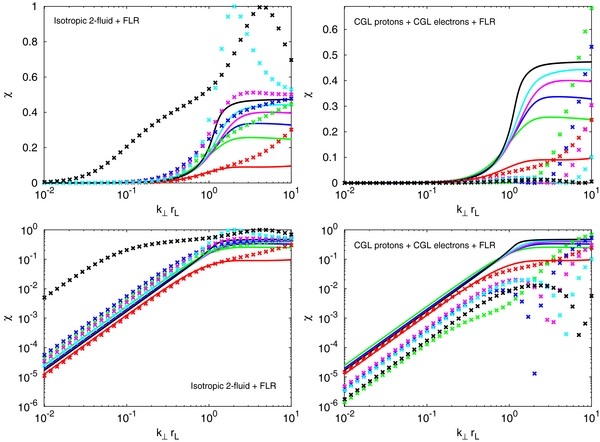
Figure 11. Compressibility χ of KAWs with θ = 8999 for the isotropic two-fluid + FLR model (left column) and the CGL proton + CGL electrons + FLR model (right column). Top panels have the χ in a linear scale, while bottom panels in a logarithmic scale. Kinetic solutions are solid lines and fluid solutions are crosses. Proton β is 0.1 (red), 0.5 (green), 1.0 (blue), 2.0 (magenta), 4.0 (cyan), and 10.0 (black).
Download figure:
Standard image High-resolution image
Figure 12. Polarization  (top) and real frequency ωr/Ωp (bottom), all parameters are the same as in Figure 11.
Download figure:
Standard image High-resolution image
All the discrepancies presented in this paper can be resolved by using a fluid model that incorporates low-frequency kinetic effects (i.e., the FLR-Landau fluid model). The FLR-Landau fluid model correctly captures both compressibility and polarization. The reason for these discrepancies is simple: kinetic effects are important and cannot be ignored even at scales much larger than proton gyroscale. This conclusion suggests that caution should be exercised in the development of theoretical and numerical descriptions that incorporate "multi-layer" physical models where the large scales are described by the equations of MHD and the small scales by a kinetic description.
P.H. was supported by NASA Postdoctoral Program, which is administered by Oak Ridge Associated Universities (ORAU). M.L.G. was supported, in part, by the Interdisciplinary Science program of the Magnetospheric Multiscale mission at the Goddard Space Flight Center. The research leading to these results has received funding from the European Commission's Seventh Framework Programme (FP7/2007-2013) under the grant agreement SHOCK (Project No. 284515). The support of INSU-CNRS "Programme Soleil-Terre" is also acknowledged. We acknowledge the partial support of NASA grants NNX08AJ33G, Subaward 37102-2, NNX09AG70G, NNX09AG63G, NNX09AJ79G, NNG05EC85C, Subcontract A991132BT, NNX09AP74A, NNX10AE46G, NNX09AW45G, and NSF grant ATM-0904007.
APPENDIX A: EQUATIONS OF FLUID MODELS
The basic equations of all the fluid models considered here (consisting of protons and electrons) are described by the following system of equations:


In the above system, the plasma is considered electrically neutral (np = ne = n) and the total plasma density is approximated by the proton density ρ = mpn. The electric current is given by j = (c/4π)∇ × B and the displacement current is neglected. The electron inertia is neglected and the electron velocity ue is directly related to the proton velocity up by ue = up − j/ne. The system is not closed and a form of the pressure tensor pr must be further specified (index r = p for protons and r = e for electrons).
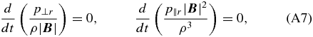
Isotropic two-fluid model. The isotropic two-fluid model is described by Equations (A1)–(A4), where the pressure tensor for both particle species is isotropic pr = prI and the scalar pressure obeys  . We used γp = 5/3 and γe = 1. For numerical solutions it is useful to write the scalar pressure equations in an explicit time-dependent form as

Anisotropic two-fluid model: CGL protons + CGL electrons. The anisotropic two-fluid with CGL protons and CGL electrons is described by Equations (A1)–(A4), where the pressure tensor for both particle species is

The  is the unit vector along the local magnetic field. The scalar parallel and perpendicular pressures obey the usual CGL condition:
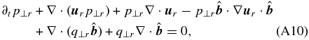
which in explicit time-dependent form is equivalent to


This model is equivalent to the LS-Landau fluid model if the heat fluxes for both particle species are neglected, i.e., q⊥r = 0 and q∥r = 0. We emphasize that after linearization and imposing isotropy for the mean pressure values  , this model is not equivalent to the linearized isotropic two-fluid model.
Anisotropic two-fluid model: CGL protons + Iso electrons. This model is used only in Figure 3. The proton pressure tensor is anisotropic according to (A6) and obeying the CGL conditions (A8) and (A9). The electron pressure is isotropic and obeys (A5) with γe = 1.
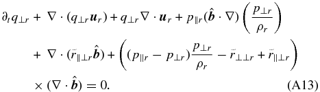
Large-scale Landau fluid model. The LS-Landau fluid model we use here is constructed from the FLR-Landau fluid model of Passot et al. (2012) by neglecting all non-gyrotropic contributions, i.e., by prescribing Π = 0,  ,
,  , and
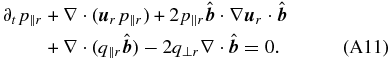
, and  . The model is described by Equations (A1)–(A4), where the pressure tensor for both particle species is anisotropic (A6) and the scalar pressures evolve according to
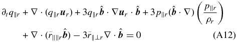
The above pressure equations contain (scalar) parallel and perpendicular heat flux components q∥r and q⊥r. The dynamics of these components is given by
The system is still not closed and the heat flux equations require expressions for the gyrotropic fourth-rank cumulants  , and
, and  . These are obtained from Equations (11)–(15) of Passot et al. (2012) by evaluating them in their large-scale limit b → 0, where the parameter
  should not be confused with the magnetic field. The final expressions are written in Fourier space and are equal to
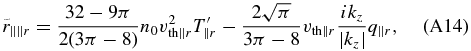
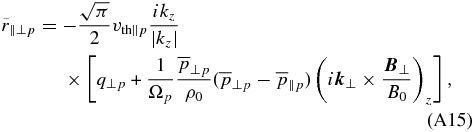
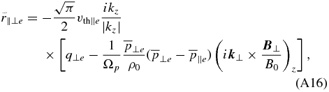

The "overline" operator (i.e.,  ) denotes instantaneous mean/averaged quantities in the entire considered (simulation) domain. Note that because no mean pressure/temperature anisotropy is considered in the present paper, i.e.,
  , the expressions (A15) and (A16) are further simplified. In the expressions (A14)–(A17), the global mean magnetic field is assumed to be in the z-direction, so kz is the parallel wavenumber. The operator ikz/|kz| describes the Landau resonance in the fluid formalism. Note that kz/|kz| is equivalent to the sign of kz and that for purely perpendicular propagation with kz = 0, there is no singularity present; the operator is just equal to zero. Equations (A14)–(A17) were derived using linear kinetic theory in the low-frequency limit and are therefore meant to be linear (i.e., directly transferable between Fourier and real space). The parallel temperature of fluctuations
  in the first term of (A14) is therefore meant to be linearized. The parallel thermal speed is defined as
  .
.
FLR-Landau fluid model. We use the FLR-Landau fluid model as described in Passot et al. (2012). The model uses Equations (A1)–(A4) with the anisotropic pressure tensor

where the Kronecker operator δrp signifies that the FLR corrections,  , to the pressure tensor are considered only for protons. The model is formulated by the gyrotropic pressure Equations (5)–(8), gyrotropic heat flux Equations (9) and (10), and equations for the gyrotropic fourth-rank cumulants (11)–(15). The FLR tensor Π is prescribed by Equations (16)–(22), where the required coefficient
  is specified in Appendix B of the same paper by Equations (B7)–(B9) and (B14). The non-gyrotropic heat fluxes
  and
and  are prescribed by Equations (23)–(28). The remaining contribution σ from the heat flux tensor only appears at the nonlinear level. The non-gyrotropic fourth-rank cumulants
  are specified by Equations (36) and (37). Coefficients containing expressions with functions Γ0(b), Γ1(b), defined as Γν(b) = e−bIν(b), where Iν is the modified Bessel function, are specified in Appendix A of the same paper.
Further notes. Equations of all the fluid models were further linearized and normalized. The normalization is done with respect to the equilibrium density ρ0 = mpn0, the magnitude of the mean magnetic field B0, the Alfvén speed vA = B0/(4πmpn0)1/2, the ion inertial length di = vA/Ωp, and the equilibrium parallel proton pressure  . The heat fluxes are normalized by
  and the fourth-rank cumulants by
  . The proton plasma beta is defined as
  , where the proton thermal speed
  . In the linear analysis presented here, the mean temperatures are not evolving and β is time-independent constant specified initially and therefore equal to
  . The equations for the isotropic two-fluid are normalized with respect to the equilibrium (isotropic) proton pressure
  and the proton plasma β is equal to
  . The proton Larmor radius
  and the proton cyclotron frequency Ωp = B0e/(mpc). Note that even though the electron inertia is neglected (i.e., the terms
  in the electron momentum equation are neglected), in Landau fluid models the electron mass me enters the equations for the gyrotropic electron heat fluxes and forth-rank cumulants. We use me/mp = 1/1836.
APPENDIX B: USUAL FLUID MODELS WITH LARGE-SCALE FLR CORRECTIONS
The first model considered here is described by Equations (A1)–(A4), where the pressure tensor pr = Ipr + Πδrp and the scalar pressures evolve according to (A5) with γp = 5/3 and γe = 1. We call this model "isotropic two-fluid + FLR." The second model is described by Equations (A1)–(A4), where the pressure tensor is given by (A18) and the scalar pressures evolve according to (A8) and (A9). We call this model "CGL protons + CGL electrons + FLR." The large-scale FLR tensor we use here is given by
Note that imposing mean pressure isotropy ( ), as is used in the present paper, further simplifies these expressions. Figure 11 shows magnetic compressibility χ of highly oblique KAWs (θ = 8999) calculated from these two models. For completeness, the χ is plotted both in a linear scale (top panels) and in a logarithmic scale (bottom panels). Figure 12 shows polarization
  (top panels) and real frequency ωr (bottom panels).
  in the isotropic two-fluid + FLR model (Figure 12, top left) for β ⩽ 2 at all range of scales. For β = {4.0, 10.0},
  at large scales and it switches to
  at small scales somewhere between k⊥rL = 2 and k⊥rl = 3. In the CGL protons + CGL electrons + FLR model (Figure 12, top right), at large scales,
  for all β except β = 0.5. For β = 0.5,
  at large scales and it switches to
  at around k⊥rL = 4. For β = {1.0, 2.0, 10.0},
  at large scales, but it switches to
  at smaller scales and later it switches back to
  at even smaller scales. The polarization is not correctly reproduced by either of these models. Moreover, the compressibility for both of these models (Figure 11) is in general different from that obtained from the kinetic calculations. The real frequency calculated from CGL protons + CGL electrons + FLR model (Figure 12, bottom right) shows the same deficiencies at sub-proton scales k⊥rL > 1 as were demonstrated for the CGL protons + CGL electrons model without the FLR corrections. We conclude that FLR corrections should not be introduced into the usual fluid models before the Landau damping is incorporated via heat flux equations.