


ABSTRACT
We develop a new diagnostic technique that utilizes, at the same time, two completely different types of observations—in situ determinations of solar wind charge states and high-resolution spectroscopy of the inner solar corona—in order to study the temperature, density, and velocity of the solar wind as a function of height in the inner corona below the plasma freeze-in point. This technique relies on the ability to calculate the evolution of the ion charge composition as the solar wind escapes the Sun given the wind temperature, density, and velocity profiles as a function of distance. The resulting charge state composition can be used to predict frozen-in charge states as well as spectral line intensities. The predicted spectra and ion charge compositions can be compared with observations carried out when spectrometers and in situ instruments are in quadrature configuration to quantitatively test a set of assumptions regarding density, temperature, and velocity profiles in the low corona. Such a comparison can be used in two ways. If the input profiles are predicted by a theoretical solar wind model, this technique allows the benchmarking of the model. Otherwise, an empirical determination of the velocity, temperature, and density profiles can be achieved below the plasma freeze-in point applying a trial-and-error procedure to initial, user-specified profiles. To demonstrate this methodology, we have applied this technique to a state-of-the-art coronal hole and equatorial streamer model.
Export citation and abstract BibTeX RIS
1. INTRODUCTION
The structure of solar wind acceleration near the Sun shapes the heliosphere and directly affects the interaction with Earth's atmosphere. It is also the best test case for acceleration processes in stellar winds that are likely near many solar-like stars. Despite this importance, we still have a lot to learn about the origin, acceleration, and evolution of the solar wind in the inner corona. Two fundamental open questions in solar wind science are: (1) From what type of plasma structures in the solar atmosphere does the solar wind originate? and (2) How is the solar wind accelerated?
It has long been known that the solar wind is divided into two qualitatively different classes: the slow solar wind, associated with streamers, and the fast solar wind, coming from open-field coronal holes (CHs; Krieger et al. 1973; McComas et al. 1998; Zurbuchen 2007). The fast wind is accelerated below 7 solar radii from solar center (Quemerais et al. 2007), and originates from the lowest altitude regions in the solar atmosphere, while slow wind comes from higher altitudes in streamers (Strachan et al. 2002). However, there is a vigorous debate on the actual location of the source of the solar wind within CHs and streamers (Kohl et al. 2006; Suess et al. 2009; Abbo et al. 2010; Antiochos et al. 2011; Antonucci et al. 2011).
Parker (1959) described the solar wind acceleration as a time-stationary process in which energy is injected into the solar wind, as it becomes supersonic. The question about the source and distribution of this energy is tied to the question of the origin of the wind. Two promising types of models of solar wind heating have been proposed: wave/turbulence-driven models and reconnection/loop opening models (Karachik & Pevtsov 2011 and references therein). Models relying on dissipation of some kind of magnetic waves differ both on the nature of the waves and on their dissipation mechanisms (i.e., Hollweg 1986; Tu & Marsch 1997; Cranmer et al. 1999, 2007; Kohl et al. 2006) and these in turn depend on the local conditions of the coronal magnetic field and plasma. Other models are based either on magnetic reconnection of open and closed magnetic field lines as a driver for coronal plasma acceleration (Fisk & Schwadron 2001) or on energy flux density and magnetic field configuration at the base of the corona (Wang & Sheeley 2003).
The two main avenues to observationally constrain proposed solar wind models are: (1) in situ measurements of solar wind plasma parameters like charge state and element composition, magnetic field, and dynamics; and (2) remote-sensing observations of the wind source regions in the inner solar corona. These two types of measurements involve very different instruments, observation techniques, and data analysis tools. When used separately, each method can provide information on only a subset of the solar wind acceleration process. For example, remote-sensing observations constrain the source region of the solar wind and their physical properties, but they can tell nothing of the final status of wind plasma after freeze-in occurs. On the other hand, in situ observations provide information on the final state of the wind plasma, but have limited diagnostic potential for its evolution near the Sun. For example, temperatures obtained through in situ measurements of ion abundance ratios under local freeze-in assumptions have limited connection with the actual temperature of the wind source regions (Landi et al. 2012a). When used together, remote-sensing and in situ observations have a great potential to study the solar wind and in its entire evolution from the source regions through the inner corona where the ionization state of the wind freezes in. However, these tools are seldom combined for analysis purposes. Such a combination usually consisted of comparisons of in situ determinations of the plasma elemental composition and electron temperature (through ion abundance ratios) with values determined spectroscopically from selected regions in the inner corona. These simple comparisons provide tools to investigate solar wind type (Zurbuchen et al. 2002), source regions (Hefti et al. 2000), and acceleration mechanisms (Gloeckler et al. 2003). However, there are two main limitations of such comparisons. First, the in situ and spectroscopic measurements being compared in many cases were not coordinated and involved unrelated observations taken at different times. Second, when coordinated observations were taken in situ and remote-sensing measurements were generally not linked; on the contrary, the comparison was limited to the measurements obtained at either side of the wind trajectory, with no insight of the evolution of the wind plasma parameters from the source region to the in situ instrumentation (see, for example, Suess et al. 2000; Poletto et al. 2002).
In the present work, we develop a new diagnostic technique that allows us to directly and quantitatively link in situ observations of ion composition obtained from time-of-flight spectrometers, such as SWICS on board Ulysses and ACE, with high-resolution spectra observed in the inner corona, such as those from the Coronal Diagnostic Spectrometer (CDS), Solar Ultraviolet Measurement of Emitted Radiation (SUMER), and Ultraviolet Coronagraph Spectrometer (UVCS) (on board the Solar and Heliospheric Observatory (SOHO)) and EIS (on board the Hinode). Such a combination exploits the strengths of both observing techniques and can be used (1) to investigate the heating and acceleration of both slow and fast solar wind, and (2) to uniquely identify the solar wind source regions. To show the potential of this technique, we apply it to testing the accuracy of a predicted temperature, density, and velocity profiles of the state-of-the-art solar wind model developed by Cranmer et al. (2007).
The new diagnostic technique is described in Section 2, and it is applied to the Cranmer et al. (2007) model using EIS and SUMER data in Section 3. Section 4 summarizes the results.
2. THE DIAGNOSTIC TECHNIQUE
2.1. The Freeze-in Process
As the solar wind plasma is accelerated, its density rapidly decreases with distance from the Sun. The fast decreasing density effectively shuts down the ionization and recombination processes, since ionization and recombination rates are directly proportional to the electron density itself. When the wind density reaches a sufficiently low value, the evolution of the plasma ionization state stops and freezes in (Hundhausen et al. 1968). Even though each element and ion in the solar wind freezes in at its own height, most of them freeze in below ≃ 5 solar radii (e.g., Ko et al. 1997; Landi et al. 2012a). Beyond that height, the wind ion composition remains unaltered regardless of the thermal and dynamic evolution the wind plasma undergoes until being detected in situ. This means that the ion composition measured by in situ instruments retains information about the physical processes it has undergone at the very beginning of its acceleration from the wind source region. Thus, such composition values can be used to gain insight on the acceleration and heating history of the plasma during the earliest stages of the wind trajectory, where it could be observed from remote.
2.2. Bridging In Situ and Remote-sensing Measurements
In situ and high-resolution spectral observations of the inner corona can be combined using an ion composition model that predicts the evolution of the ion abundances of wind plasma leaving the Sun from the source region to the freeze-in point and beyond to Earth. This model solves the time-dependent equation for ionization and recombination for a chosen element as it travels outward from the Sun:

where Te is the electron temperature, ne is the electron density, Ri and Ci are the total recombination and ionization rate coefficients, and ym is the fraction of the element X in charge state m. The set of continuity equations for each element is solved numerically as a set of stiff ordinary differential equations using a fourth-order Runge–Kutta method (Press et al. 2002). To ensure computational efficiency, the step size is set adaptively and the accuracy of the integrator is tested to ensure high accuracy (better than 10−6).
The solution provides the values of the charge state composition of the solar wind plasma at all places from the source region to the freeze-in point (beyond which, charge states are constant). Such a code requires three main ingredients.
- 1.The temperature, density, and velocity of the plasma as a function of distance from the source.
- 2.A complete database of ionization and recombination coefficients.
- 3.The assumption of local thermodynamic equilibrium in the wind source region, as a boundary condition.
Examples of these codes are those developed by Ko et al. (1997) and Gruesbeck et al. (2011). Both these codes solved Equation (1), but they used different ionization and recombination rate coefficient: Gruesbeck et al. (2011) used the compilation by Mazzotta et al. (1998), while Ko et al. (1997) used a combination of data taken from multiple sources in the literature available at the time (see Ko et al. 1997 for details). Also, Gruesbeck et al. (2011) applied Equation (1) to the calculation of charge states in the core of a coronal mass ejection (CME), using an ad hoc temperature profile during the initial heating of the CME plasma until a height rheat, beyond which the temperature evolution followed the equations for adiabatic expansion; the adiabatic expansion was also used to calculate the density decrease with distance. Ko et al. (1997), on the contrary, applied Equation (1) to the calculation of charge states in the fast solar wind, using an empirically determined density profile, and a parametric form of the electron temperature and wind velocity; they determined the parameters for the electron temperature as the values that allowed the predicted frozen-in charge states resulting from Equation (1) to best match the observations.
In the present work, we use the Gruesbeck et al. (2011) code to calculate the charge state evolution of the plasma in the fast and slow solar wind, by using as input the temperature, density, and velocity profiles predicted by the Cranmer et al. (2007) model. The predicted charge state evolution serves as a bridge between ion composition measurements anywhere in the heliosphere and spectral lines intensities in the low corona because
- 1.at one end of the wind trajectory, the frozen-in charge state distribution for a given element can be directly compared with in situ observation, in a similar way as done by Ko et al. (1997); and
- 2.
These two quantitative comparisons can be used in two different ways. On one side, if the temperature, density, and velocity profiles are taken from a theoretical solar wind model, the comparison allows a thorough, end-to-end benchmark of the predictions of the model. On the other side, an empirical determination of the best temperature, density, and velocity profiles can be obtained through a trial-and-error process: first, a particular form of such profiles (guided by spectroscopic or white light measurements where available) is assumed and the charge state evolution is calculated; second, the results are compared both with the in situ measurements and spectral line intensities. The comparison is then used as a guide to modify the assumed profiles: this procedure can be repeated using the modified profiles until agreement is achieved.
Key to both these types of quantitative comparison is the fact that each ion and element freezes in at a different height, so that including as many elements and ions as possible in this process is important in order to achieve a thorough sampling of the entire freeze-in region and the best diagnostics of the nascent solar wind properties.
Note that such a comparison can in principle be extended also to time-transient conditions, such as those in CME ejecta, and thus can be a very powerful tool to determine the heating and thermal history of CME plasma in the lower solar atmosphere. For example, groundbreaking results in CME studies have already been obtained by Gruesbeck et al. (2011) just using in situ measurements.
2.3. Comparison with In Situ Observations
Comparison of in situ ion charge measurements with the results of the ionization code is straightforward, as the frozen-in ion abundances calculated by the latter can be directly matched to their observed counterparts.
2.4. Comparison with High-resolution Spectra
The predictions of individual ion abundances made by the ionization code allow the calculation of individual line intensities as a function of height above the solar limb. In fact, the intensity (in erg cm−2 s−1 sr−1) of a spectral line emitted by a transition from level j to level i of ion X+q is given by
where Te is the electron temperature, dT and dx lie along the line of sight, a includes atomic constants involved in the radiation absorption process, Finc is the intensity of the incident radiation, p(ϕ) is the scattering factor, and D(v) is the Doppler dimming term (see Beckers & Chipman 1974; Noci & Maccari 1999; Phillips et al. 2008 for a definition). The line contribution function Gji(Te, ne) and the number of absorbers Nabs are defined as
where nj(X+q)/n(X+q) is the relative population of the upper level j of the ion X+q, n(X+q)/n(X) is the relative abundance of the ion X+q, n(X)/n(H) is the abundance of X relative to hydrogen, n(H)/ne is the hydrogen density relative to that of free electrons ne, Aji is the Einstein coefficient for spontaneous emission, h is the Planck constant, and νji is the transition frequency. Close to the corona, Irad ≪ Icoll for the majority of spectral lines, but for a few of them emitted in the visible its contribution is significant or even dominant already as low as 1.1 Rsun (e.g., Habbal et al. 2011), and thus needs to be taken into account.
The output of the ionization code provides the missing ingredient for the calculation of spectral line intensities. In fact, the electron density and temperature curves used as input to the ionization code can be combined with the CHIANTI spectral code to calculate the relative level population nj(X+q)/n(X+q) at all places along the wind trajectory; the ionization code predictions of the relative ion abundance n(X+q)/n(X) and the elemental abundance n(X)/n(H) measured by in situ instrumentation can be used for both Icoll and Irad. The scattering function p(ϕ) can be calculated for any transition according to House (1970). Thus, the emissivity of any spectral line of each ion can be calculated at all places along the trajectory of the wind plasma. When some assumption on the distribution of the plasma along the line of sight is made, usually based on available narrowband imagers such as SOHO/EIT, TRACE, STEREO/EUVI, SDO/AIA or Hinode/XRT, the expected absolute line intensity profile with distance can be calculated and compared with the observed one.
The predicted line intensities can be compared to observed spectra in two ways: first, the curve normalized to the innermost value can be compared with normalized intensity profiles measured by high-resolution spectrometers outside the solar limb. Such curves allow us to compare the rate of decrease of predicted intensity of lines from different ion species and allow us to test the evolution of consecutive ion stages as a proxy of wind plasma heating and boundary conditions. Second, absolute line intensities can be used to test the accuracy of the assumed electron density, plasma distribution along the line of sight, and of the boundary conditions in the source regions.
It is important to note that the present technique can in principle be applied also to intensities measured by narrowband imagers such as SOHO/EIT, TRACE, Hinode/XRT, STEREO/EUVI, and SDO/AIA. In fact, Equation (3) can be used to predict the entire spectrum included in the instrument passband, to be folded through the imager's effective area. The downside of the use of imagers is that the intensities of lines from many different ions are averaged together, so that the diagnostic potential of each of them gets mixed and the overall sensitivity of the diagnostic technique to changes in the input model is somehow decreased.
2.5. Suitable Observations
The double comparison outlined above can only be applied to observations that meet certain requirements. First, predicted line intensities need to be compared to intensity measurements made as a function of height above the photosphere in the wind source region. Thus, this diagnostic technique requires spectral observations taken at the solar limb, with the spectrometer field of view covering as much distance from the limb as possible. In contrast, observations on the disk are not suitable because they are dominated only by the lowest (and brightest) regions of the solar corona and do not allow us to measure the intensity profile as a function of height above the limb.
Second, the full potential of this technique can be exploited only when in situ and spectroscopic observations of the same plasma parcel are used. Since the spectrometers used in such a study need to be pointed at the solar limb, this can only be achieved under quadrature conditions: in this case, spectroscopic observations at the limb along the direction connecting the Sun and the in situ instrument will point the same plasma that will be later detected by the latter.
In the case of polar CHs during minimum, meaningful comparisons can still be done on data sets taken outside quadrature capitalizing on the fact that during solar minimum the properties of the fast solar wind are remarkably constant. In this case, spectral observations at the limb of polar CHs not directly connected with any particular in situ measurement can still be combined with the average values of in situ fast wind charge state composition.
In case a combination of in situ and spectroscopic data sets is not available, the technique we propose in this work can also be applied when only one of them is available. For example, Gruesbeck et al. (2011) applied the ionization code predictions to determine the physical properties and evolution near the Sun of a CME using only their ion composition observed by the ACE/SWICS spectrometer near the Earth; however, no measurements were available from spectrometers near the Sun. Landi et al. (2012c), on the contrary, used the spectroscopic measurements of the physical properties of the ejecta of the CME launched on 2008 April 9 to predict the evolution of its ejecta as the CME traveled through space; being a limb event, such predictions could not be compared with in situ observations, but helped illustrate the origin of typical in situ compositional features of CME ejecta.
2.6. Strengths of This Technique
The main strength of this technique relies on using two entirely different sets of observables to test the validity of assumed wind velocity, temperature, and density. The number of constraints that are posed by line intensities near the Sun, and frozen-in charge states far from the Sun, is formidable.
In fact, different ions and elements react to wind-induced changes in the plasma density and temperature in a very different way, because their ionization and recombination rate coefficients have wildly different values. In general, lighter elements tend to freeze-in very close to the Sun (Landi et al. 2012a) while ions from heavier elements evolve for a longer time as they travel away from the Sun (Ko et al. 1997). As a consequence, their line intensities will be affected by the wind at different (but often partially overlapping) heights, and to different extents. Frozen-in charge states allow the further extension of this benchmark to regions not easily accessible to spectrometers, so that the final stages of the wind plasma evolution can also be tested.
Finding a set of velocity, density, and temperature profiles that reproduces both kind of measurements is very difficult. For example, different combinations of plasma velocity and temperature may provide an equally acceptable fit to in situ measurements of frozen-in charge states for a given element; still, they will cause the ionization of such elements to evolve very differently close to the Sun, so that the resulting intensity profiles of lines emitted close to the Sun will change considerably and therefore can be used to narrow down the allowable profiles. Comparison with observed spectra can determine which velocity and temperature combination agrees with both in situ and spectral data. Hence, this diagnostic technique is best suited for spectra including lines emitted by a large number of ions, as well as to in situ charge state measurements from different elements.
Another strength of this technique is that in principle it can also be applied to CME plasmas. In fact, after the temperature, density, and velocity profiles are specified by a CME model for any portion of the CME plasma, the charge state evolution for all relevant elements can be calculated and compared with in situ measurements and spectral line intensities (or even narrow band images) in the same way as the solar wind.
2.7. Limitations of This Technique
There are a few assumptions underlying this diagnostic technique that need to be considered. First, the ion composition models such as those developed by Ko et al. (1997) and Gruesbeck et al. (2011) rely on the assumption that the plasma electron distribution is Maxwellian, or at least not significantly different from it. While this may be a good approximation in the innermost regions of the solar corona, departures from Maxwellian distributions are expected to occur fairly soon along the solar wind trajectory (e.g., Marsch 2006 and references therein). Non-Maxwellian electron velocity distributions can alter quite significantly the available ionization and recombination rate coefficients, since the latter are usually calculated assuming a Maxwellian distribution (Owocki & Scudder 1983). Departures from Maxwellian distributions do not constitute a problem if they occur after the freezing point, but may lead to incorrect in situ and line intensity predictions that can limit the accuracy of the diagnostic results if they are non-negligible before the freeze-in point.
Another limitation of this technique lies in the implicit assumption made by the ionization code that all elements have the same dynamic evolution. For example, Kohl et al. (2006) indicate several instances where UVCS observations indicate that the proton and oxygen speeds are significantly different in the early stages of solar wind acceleration; Byhring et al. (2011) showed through numerical models that decrease in Coulomb coupling between iron ions and hydrogen caused the former to have a slower speed than the latter; they also showed that each ion decoupled its velocity from hydrogen at a different height due to the different values of Coulomb cross sections. The presence of different velocity profiles for each element in the inner corona will lead to, if all elements are considered together, significant confusion in the interpretation of the predicted-to-observed comparison. If, on the contrary, each element is allowed to have its own velocity profile, the diagnostic potential of this technique will be somewhat limited because the velocity curve of each element can be determined only in the height range before this element freezes in.
The ionization codes developed so far calculate the evolution of a single-temperature plasma. This assumption is, however, not strictly accurate. In fact, while the thermal distribution of CH and quiet-Sun plasmas have been consistently found to be close to isothermal (Feldman & Landi 2008 and references therein), nonetheless small amounts of plasma at either side of the plasma main temperature have been unambiguously identified both in CHs (Hahn et al. 2011) and in quiet Sun (Warren & Brooks 2009; Landi & Young 2010). The presence of small tails of cold and hot plasma in the inner corona can alter the initial plasma ion composition taken as a boundary condition by ionization models.
Another source of uncertainties is the distribution of plasma along the line of sight close to the Sun, i.e., whether structures with different physical properties (like CHs and streamers) are simultaneously present along the integration path. Incorrect assumptions on the plasma distribution may lead to incorrect predicted line intensities in Equation (3). These uncertainties can be minimized in two ways. First, the distribution of plasma structures can be empirically determined using narrowband images of the solar disk and corona in white light or EUV. Such an approximate determination can capture the main features of the plasma along the line of sight. Second, a more accurate determination can be achieved using three-dimensional tomographic reconstructions of the solar corona from a series of white light or EUV narrow bandpass images (Frazin et al. 2009).
3. APPLICATION
The systematic application of the diagnostic technique to benchmark theoretical models, or to empirically determine the solar wind properties, is beyond the scope of the present work. Here, we only show an example of its application to a state-of-the-art theoretical model of the fast and slow solar wind from Cranmer et al. (2007).
3.1. Theoretical Model
We use temperature, density, and velocity profiles from the solar wind model of Cranmer et al. (2007). This is a self-consistent model of the photosphere, chromosphere, corona, and solar wind mainly driven by MHD turbulence, and it provides the plasma properties along open magnetic flux tubes rooted in solar CHs, streamers, and active regions. At the base of this model the plasma is assumed to be in ionization equilibrium. Cranmer et al. (2007) predicted the plasma bulk speed, temperature, and density along magnetic field lines: we considered here examples for the CH and the equatorial streamer (EQ) kindly provided by the authors. These are taken as proxies for the fast and slow wind, respectively. The density, temperature, and velocity profiles predicted by Cranmer et al. (2007) for both plasmas are shown in Figure 1.
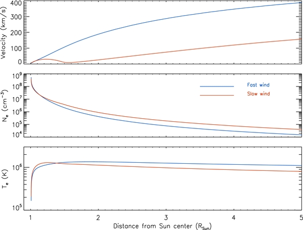
Figure 1. Input theoretical model for the plasma electron temperature Te, electron density Ne, and outflow speed v along an open magnetic flux line in a coronal hole (blue, for the fast solar wind) and a streamer (red, for the slow solar wind) as a function of distance from the solar center from Cranmer et al. (2007).
Download figure:
Standard image High-resolution imageFor simplicity, we assume in our calculations that the plasma velocity, density, and temperature only depend on distance from the Sun center everywhere in the corona. Such an assumption is taken for both the CH and the streamer models of Cranmer et al. (2007). Such a simplistic approximation is taken only to illustrate the diagnostic technique, and not to validate the Cranmer et al. (2007) model; a thorough benchmark of the model requires more realistic assumptions of the plasma distribution and will be done in a future work.
All ionic charge states freeze in as the electron density decreases by several orders of magnitude. Beyond the freeze-in point, the solar wind can undergo tremendous dynamic evolution, but the ionic charge states do not change. Thus, our calculations were stopped at ≈15 Rsun, when all ionic species in the wind are frozen in. Examples of the evolution of carbon, oxygen, and iron charge states as a function of distance from the solar surface are shown in Figures 2 and 3, which report the ratio of each ion abundance to its final frozen-in value. Both the CH and EQ cases are shown. The slower speed and the larger electron density cause the slow wind ion abundances to freeze in at larger distances than in the fast wind.

Figure 2. Ratio of the predicted ion abundances to their frozen-in value calculated at 15 Rsun in the fast solar wind for carbon (left, red curve), oxygen (left, blue curve), and iron (right) ions. Black horizontal dashed lines indicate where the predicted ion abundances are within 10% of their frozen-in values.
Download figure:
Standard image High-resolution image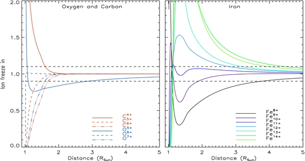
Figure 3. Ratio of the predicted ion abundances to their frozen-in value calculated at 15 Rsun in the slow solar wind for carbon (left, red curve), oxygen (left, blue curve), and iron (right) ions. Black horizontal dashed lines indicate where the predicted ion abundances are within 10% of their frozen-in values.
Download figure:
Standard image High-resolution image3.2. Observations
In order to compare the predictions from the Cranmer et al. (2007) model with observations, we used observed spectral line intensities from both CHs and streamers, as well as in situ measurements of ion abundances from ACE/SWICS. It is important to note that the spectral and in situ data were not correlated, and they have been chosen only to provide comparison examples and illustrate the main features of the diagnostic technique, and not to benchmark the model itself. A future work will be devoted to carry out a much more detailed comparison using a set of observations that satisfy the requirements outlined in Section 2.5.
Table 1 lists the specific parameters of the observations. We focused on EIS (Culhane et al. 2007) and SUMER (Wilhelm et al. 1995) because both instruments can observe the innermost regions of the solar corona (their field of view includes the entire solar disk and stretches up to approximately 1.35–1.50 Rsun depending on the instrument pointing, where the solar limb is taken at 1.0 Rsun), and their spectral ranges include a number of bright, isolated spectral lines that can be observed with sufficient signal to noise for the entire length of the instruments' slits.
Table 1. Details of the SOHO/SUMER and Hinode/EIS Used in This Work
| Polar Coronal Hole | Equatorial Streamer | ||
|---|---|---|---|
| SUMER | EIS | SUMER | |
| Date | 1996 Nov 3 | 2009 Apr 25 | 1996 Nov 21 |
| Slit center | (0'',1150'') | (0'',−1120'') | (1160'',0'') |
| Field of view | 2'' × 300'' | 2'' × 512'' | 4'' × 300'' |
| Raster | No | No | No |
| Slit width | 2'' | 2'' | 4'' |
| Height (Rsun) | 1.03–1.34 | 0.87–1.47 | 1.03–1.34 |
| Exposure time (s) | 1200 | 600 | 3000 |
| Spectral range (Å) | 50–1500 | 170–212, 246–292 | 500–1500 |
Download table as: ASCIITypeset image
The common feature of the observations listed in Table 1 is that their field of view stretches radially from the solar limb outward; also, the exposure time was large in all three cases. This allowed us to measure the intensity of spectral lines as a function of distance from the limb for as high as allowed by each instrument. All data were cleaned and calibrated using the standard data reduction software available in SolarSoft for both instrument. For the EIS instrument, the software allows for dark current, cosmic ray; hot, warm, and dusty pixel removal; correction of the long-term CCD degradation; slit tilt and misalignment between the two EIS detectors. SUMER data were decompressed and corrected from geometrical distortion of the CCD image and the flat field. Both SUMER and EIS data were averaged in 10 pixel bins along the slit direction to increase the signal-to-noise ratio; such rebinning decreases the spatial resolution along the slit to approximately 0.01 Rsun bins. Absolute line intensities were measured in photons cm−2 s−1arcsec−2. The signal-to-noise ratio of the averaged intensities is large so that uncertainties are dominated by the uncertainty in the EIS and SUMER absolute calibration, 22% (Lang et al. 2006) and 20% (Schühle et al. 2000), respectively.
Since we are interested in off-disk observations, instrument-scattered stray light is an important issue as it can contaminate the real coronal emission at large heights, where local line emission is weakest. We have accounted for stray light correction of SUMER line intensities using the method outlined by Feldman et al. (2006). In EIS, we have determined the contribution of the instrument scattered light as 2% of the intensity observed in the portions of the EIS slit observed inside the solar disk, as suggested by Ugarte Urra (2010). Since the lines we selected as examples are bright, scattered light was negligible below 1.35 Rsun; also, count rates are small beyond this height so we limited the comparison between observed and predicted line intensities up to 1.35 Rsun. The only exceptions are Mg viii 772.6 Å, Si x 624.7 Å, and Fe xi 1467.1 Å observed by SUMER, whose intensity was still dominated by scattered light at heights lower than 1.35 Rsun. For these lines, we only retained the heights where scattered light was 10% or less of the measured intensity.
In situ measurements of ion abundances were taken as averages of ion abundances measured by the ACE/SWICS instrument (Gloeckler et al. 1998) in the slow and fast solar wind over four years between 2007 and 2010. Fast wind measurements were selected as the median of all measurements where the wind speed was larger than 600 km s−1, and the O7 +/O6 + ion abundance ratio was lower than 0.1, as suggested by Zurbuchen et al. (2002). Slow wind measurements were taken as the median of all measurements where the wind speed was lower than 500 km s−1 and 0.1 ⩽ O7 +/O6 + ⩽ 1.0, again following Zurbuchen et al. (2002). Resulting ion charge state values are listed in Table 2.
Table 2. Average Charge State Abundances in the Fast and Slow Solar Wind, as Measured by ACE/SWICS During 2007–2010
| Element | Ion | Fast Wind | Slow Wind | Element | Ion | Fast Wind | Slow Wind | |
|---|---|---|---|---|---|---|---|---|
| C | 4+ | 0.478 | 0.164 | Si | 6+ | 0.114 | 0.052 | |
| 5+ | 0.456 | 0.397 | 7+ | 0.339 | 0.209 | |||
| 6+ | 0.061 | 0.439 | 8+ | 0.336 | 0.277 | |||
| 9+ | 0.171 | 0.317 | ||||||
| O | 6+ | 0.953 | 0.839 | 10+ | 0.030 | 0.112 | ||
| 7+ | 0.010 | 0.131 | ||||||
| Fe | 7+ | 0.074 | 0.047 | |||||
| Ne | 6+ | 0.148 | 0.086 | 8+ | 0.283 | 0.216 | ||
| 7+ | 0.288 | 0.295 | 9+ | 0.331 | 0.303 | |||
| 8+ | 0.565 | 0.616 | 10+ | 0.167 | 0.244 | |||
| 11+ | 0.055 | 0.127 | ||||||
| Mg | 6+ | 0.220 | 0.020 | |||||
| 7+ | 0.136 | 0.053 | ||||||
| 8+ | 0.235 | 0.115 | ||||||
| 9+ | 0.372 | 0.400 | ||||||
| 10+ | 0.037 | 0.412 |
Note. See the text for details.
Download table as: ASCIITypeset image
3.3. Comparison Results
To outline the main features of the diagnostic technique, we have compared three quantities: the predicted and observed absolute line intensities, the predicted and observed normalized line intensities, and the frozen-in charge states. For comparison purposes, we also calculated line intensities replacing the ion abundances calculated by the ionization code with ionization equilibrium values. The comparison between the two types of intensities allows us to assess the importance of wind-induced plasma departures from ionization equilibrium on spectral line intensities: such departures constitute one of the main wind diagnostic features of spectral lines.
3.3.1. Absolute Line Intensities
Absolute line intensities calculated for a sample of lines under CH and EQ conditions are shown in Figures 4 and 5, respectively. We used CH data from EIS observations, while the streamer data are taken from SUMER observations. The measured intensities of the two CH lines are very well reproduced by the Cranmer et al. (2007) model up to 1.3 Rsun; after that point, observed intensities are larger than predicted in the case of the Fe x 184.53 Å line, while slightly lower in the case of the Fe xi 188.21 Å line. The model's underestimation of the Fe x 184.53 Å line can be due to an underestimation of the Fe x ion abundance beyond 1.3 Rsun: Figure 2 shows that the Fe xi (Fe10 +) ion abundance is the first to reach its final frozen-in value at approximately 1.3 Rsun after increasing from the initial values at the lower boundary, so that it is possible that the Fe x freeze-in point is predicted to occur too early. It is worth noting that for these two ions the intensities obtained with the model ion abundances are very close to ionization equilibrium values, with the exception of the lowest heights, where the model provides better agreement with the observed intensities than the equilibrium conditions for the Fe xi 188.21 Å line.
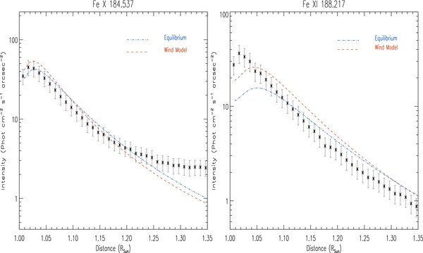
Figure 4. Observed and predicted absolute line intensity profiles in a coronal hole. Measurements have been acquired by the EIS spectrometer (stars). Theoretical density, temperature, and velocity profiles are taken from the Cranmer et al. (2007) CH model. The red line indicates calculations made using the predicted ion abundances; blue lines are calculated assuming ionization equilibrium at all places, for comparison purposes. Left: Fe x 184.53 Å. Right: Fe xi 188.21 Å.
Download figure:
Standard image High-resolution image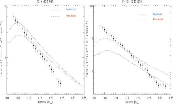
Figure 5. Observed and predicted absolute line intensity profiles in an equatorial streamer. Measurements have been acquired by the SUMER spectrometer (stars). Theoretical density, temperature, and velocity profiles are taken from the Cranmer et al. (2007) EQ model. The red line indicates calculations made using the predicted ion abundances; blue lines are calculated assuming ionization equilibrium at all places, for comparison purposes. Left: Si x 624.73 Å. Right: Fe xii 1242.02 Å.
Download figure:
Standard image High-resolution imageThe predicted absolute line intensities in the case of the EQ show some disagreement from the observed values. Figure 5 shows the intensities of the Si x 624.73 Å and Fe xii 1242.02 Å as measured by the SUMER spectrometer. These two ions are predicted to be formed at approximately the same temperature under equilibrium conditions, but the outflow speed of the slow solar wind, as well as the boundary conditions of the model, causes Fe xii to experience larger departures from equilibrium conditions than Si x. The main difference between the predicted and observed intensities in Figure 5 lies in the rate of decrease with height of both line intensities: in both cases, observed intensities drop faster than predicted. This can be due to the plasma ionizing faster than predicted as the solar wind leaves its source region.
3.3.2. Relative Line Intensities
Figures 6 and 7 compare the normalized line intensity profiles for a sample of lines observed in CHs and streamer conditions. We used CH observations from both SUMER and EIS, while the streamer data are taken from SUMER observations only. Both predicted and observed line intensities are normalized to their maximum values (which can occur at different heights), to better compare the rate of decrease (or increase) of line intensities as a function of distance.
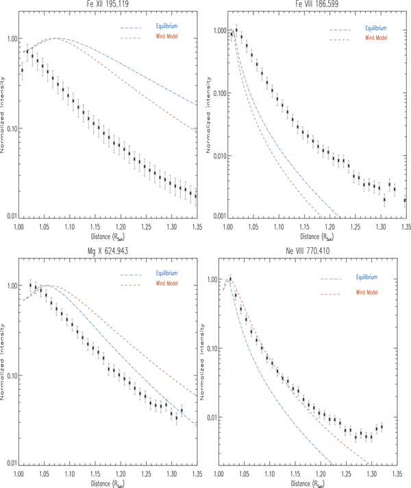
Figure 6. Normalized line intensity profiles for several lines observed by EIS and SUMER in coronal holes. Theoretical density, temperature, and velocity profiles are taken from the Cranmer et al. (2007) CH model. The red line indicates calculations made using the predicted ion abundances; blue lines are calculated assuming ionization equilibrium at all places, for comparison purposes.
Download figure:
Standard image High-resolution image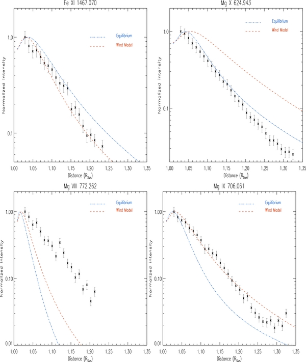
Figure 7. Normalized line intensity profiles for key lines observed by EIS and SUMER in streamers. Theoretical density, temperature, and velocity profiles are taken from the Cranmer et al. (2007) EQ model. The red line indicates calculations made using the predicted ion abundances; blue lines are calculated assuming ionization equilibrium at all places, for comparison purposes.
Download figure:
Standard image High-resolution imageNote that in both Figures 6 and 7 the intensities are calculated with the predicted ion abundances and with the equilibrium values are significantly different, by factors two or more, already at 1.1 Rsun. This shows that (1) the assumption of ionization equilibrium breaks down already at very low heights, commonly observed by spectrometers when pointed outside the solar limb, and (2) line intensities can be a powerful indicator of the effects of solar wind acceleration very close to the limb, and thus are very promising diagnostics of solar wind source regions as well as solar wind acceleration.
Figure 6 shows a few more interesting features. The intensity profile of the Ne viii 770.41 Å is reproduced nicely using the predicted ion abundances, while the equilibrium values lead to underestimate it at almost any height. The intensity profiles of all other lines, on the contrary, are not well reproduced by either assumption. Disagreements are found in the location of the peak intensity of the line, as well as in the rate of intensity decrease. The wrong position of the peak, clearly visible in the Mg x and Fe xii line intensities, indicates that Mg and Fe are too slow at ionizing from the boundary conditions (set at transition region temperatures) to those ionization stages. Since both ion abundances sets show the same feature, this can be due to two reasons: the assumed wind speed may be too fast (leaving to Mg and Fe little time to spend in the densest regions of the CH and get ionized) or the boundary temperature value is too low, so that Mg and Fe have not enough time to ionize from the boundary ion charge states to the coronal ones so that the source region of the wind is to be found at higher temperature/altitude. It is interesting to note, however, that the predicted rate of intensity decrease after the peak of both lines is in agreement with the observed one, possibly indicating that the main problem is the source region temperature. On the contrary, the position of the peak intensity of Fe viii agrees with observations, but the predicted rate of decrease is too fast. The reasons for this might be either that the temperature of the source region is too low (as for Mg x and Fe xii disagreements) or that the wind density is too high, leaving no time to Fe to spend in its 7 + charge state.
Disagreements are less striking in Figure 7, which shows the normalized intensity profiles obtained from the EQ model. The worst case is shown by the Mg viii line, whose predicted intensity profile decreases much faster than observed; the predicted ion abundances provide values closer to observations, but still the disagreement reaches one order of magnitude. Mg ix and Fe xi, on the contrary, are reasonably well reproduced with the predicted ion abundances, while the equilibrium ones fail for Mg ix. Interestingly, Mg x behaves in the opposite way, as the intensity decrease predicted with the predicted abundances is much slower than observed. In all cases, the departures of the predicted line intensities from the values expected in ionization equilibrium clearly indicates them as tools for solar wind diagnostics.
3.3.3. In Situ Charge State Measurements
On the other side of the solar wind trajectory, comparison with observations is more straightforward, as shown in red in Figures 8 and 9. Observed ion charge states are shown in the bottom row of both figures, and clearly indicate that the average charge state for all elements is larger in the slow solar wind than in the fast one. The same qualitative behavior is reproduced by the model predictions shown in blue in the top rows. However, a more detailed comparison shows non-negligible differences in all elements larger than both the estimated uncertainty of individual charge state measurements (25% or less, depending on the species) and the 1σ deviation of the averages in Table 2. For example, oxygen is predicted to be almost completely in its He-like state (O6 +), while observations indicate non-negligible tails in the two adjacent ionization stages. The neon He-like charge state (Ne8 +) is also predicted to be dominating this element, still observations indicate a more mixed composition. Also, predicted carbon charge states are shifted toward lower ionization than observed. Since C, O, and Ne freeze in at the lowest heights in the solar wind trajectory, these results indicate that corrections are needed to the velocity, density, and temperature profiles closest to the solar wind source regions. In particular, it seems that the wind plasma temperature in the source regions needs to be larger; this can be achieved either by a steeper temperature gradient and larger maximum temperature at low heights, or by a larger temperature at the model boundary, indicating a source region closer to the solar corona. Similar results are shown by the heavier elements, whose freeze-in height is larger than C, O, and Ne: they indicate that the plasma temperature may be larger than assumed.
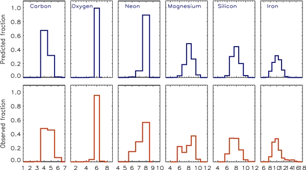
Figure 8. Predicted (top) and observed (bottom) ion charge states in the fast solar wind after freeze-in has been established. Observations are from ACE/SWICS (see the text for details), and the theoretical model has been taken from the coronal hole model by Cranmer et al. (2007).
Download figure:
Standard image High-resolution image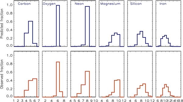
Figure 9. Predicted (top) and observed (bottom) ion charge states in the slow solar wind after freeze-in has been established. Observations are from ACE/SWICS (see the text for details), and the theoretical model has been taken from the streamer model by Cranmer et al. (2007).
Download figure:
Standard image High-resolution image
4. CONCLUSIONS
In the present work we proposed a new diagnostic technique that utilizes simultaneously two completely different types of observations—in situ determinations of solar wind charge states and spectroscopy of the inner solar corona—and combines them with a solar wind ionization model, in order to study the temperature, density, and velocity of the solar wind as a function of height from the source regions of the solar wind to Earth and beyond.
This technique relies on the ability to calculate the ion charge composition of the solar wind as the plasma flows outward from the Sun, and uses it to predict both spectral line intensities in the inner corona, and frozen-in charge states at 1 AU and beyond. The calculation is carried out once the density, temperature, and velocity profiles of the wind are given as input to the composition model. The comparison with observations can be used in two ways. First, if the input profiles are predicted by a theoretical solar wind model, this technique allows us to test them against spectra and in situ measurements to determine whether the wind model predictions are realistic. Otherwise, by using a trial-and-error procedure, an empirical determination of the velocity, temperature, and density profiles can be achieved below the plasma freeze-in point.
We have applied this technique using the temperature, density, and velocity profiles predicted by the CH and EQ models of Cranmer et al. (2007). This comparison by no means is, nor was intended to be, conclusive on the quality of the model, since the observations we used do not fulfill the requirements outlined in Section 2.5 to be used with the present diagnostic technique, and it was made for demonstrative purposes only. A more complete study with suitable observations will be made in a future work. We show that several changes to the input curves can be made in order to achieve satisfactory agreement. Also, we show that line intensity profiles depart from those obtained using the common ionization equilibrium assumption. Such departures are due to the wind velocity, and thus make it possible to use spectral line intensities for wind diagnostics, although interpretation is complicated by any inaccuracies in the assumptions of Maxwellian electron velocity distribution, of the same velocity pattern for all ionic species, and by the presence of multiple plasma structures along the line of sight.
This technique is best used with observations carried out when the inner corona spectrometers and the in situ instrumentation are in quadrature, since in this way the same plasma can be observed by both sets of instruments. However, observations carried out outside quadrature of more stationary wind conditions like in the fast solar wind can also be used.
The work of E.L. is supported by the NNX11AC20G, NNX10AM17G, and NNX10AQ58G NASA grants to the University of Michigan, and grant SV1-81002 to the Smithsonian Astrophysical Observatory. J.R.G. is supported by the GRSP program through grant NNX10AM41H. T.H.Z. and S.T.L. are supported by NASA through contract NNX08AI11G and grants NNX07AB99G and NNX10AQ61G. The authors thank Dr. S. R. Cranmer for kindly providing the theoretical temperature, density, and velocity profiles used in this work, and the referee for the valuable comments that helped us improve the paper.