


ABSTRACT
The solar atmosphere is structured and inhomogeneous, both horizontally and vertically. The omnipresence of coronal magnetic loops implies gradients of the equilibrium plasma quantities such as the density, magnetic field, and temperature. These gradients are responsible for the excitation of drift waves that grow both within the two-component fluid description (both in the presence of collisions and without it) and within the two-component kinetic descriptions (due to purely kinetic effects). In this work, the effects of the density gradient in the direction perpendicular to the magnetic field vector are investigated within the kinetic theory, in both electrostatic (ES) and electromagnetic (EM) regimes. The EM regime implies the coupling of the gradient-driven drift wave with the Alfvén wave. The growth rates for the two cases are calculated and compared. It is found that, in general, the ES regime is characterized by stronger growth rates, as compared with the EM perturbations. Also discussed is the stochastic heating associated with the drift wave. The released amount of energy density due to this heating should be more dependent on the magnitude of the background magnetic field than on the coupling of the drift and Alfvén waves. The stochastic heating is expected to be much higher in regions with a stronger magnetic field. On the whole, the energy release rate caused by the stochastic heating can be several orders of magnitude above the value presently accepted as necessary for a sustainable coronal heating. The vertical stratification and the very long wavelengths along the magnetic loops imply that a drift-Alfvén wave, propagating as a twisted structure along the loop, in fact occupies regions with different plasma-β and, therefore, may have different (EM–ES) properties, resulting in different heating rates within just one or two wavelengths.
Export citation and abstract BibTeX RIS
1. INTRODUCTION
Observations and theoretical studies in the past 70 years have dramatically increased our knowledge and understanding of the physical processes in the solar atmosphere. However, the basic starting puzzle of the problem of coronal heating still remains elusive in spite of the obvious progress made in the domain. In fact, new data collected in the course of decades have additionally increased the complexity of the problem as more and more fine details related to the heating have emerged. These include the preferential heating of plasma particles in the direction perpendicular to the magnetic field vector, resulting in a temperature anisotropy (Li et al. 1998; Cuseri et al. 1999), and the preferential heating of heavier particles. As a matter of fact, heavier ions appear to be hotter than lighter ions, while the latter on the other hand appear to be hotter than electrons (Cranmer et al. 2008). Moreover, extremely strong electric fields (above 100 kV m−1) have been detected (Zhang & Smartt 1986). Those electric fields accelerate particles and, in general, the distribution functions of the plasma species in the outer solar atmosphere can be considerably different from a Maxwellian distribution (Vasyliunas 1968; Cranmer 1998).
In our recent papers (Vranjes & Poedts 2009a, 2009b, 2009c, 2009d) a novel approach and a new paradigm for the coronal heating has been put forward. The model is based on the drift-wave theory, a well-known subject in the general plasma theory, in laboratory plasma physics, and even in terrestrial ionospheric research (Kelley 1989). Yet, the drift-wave theory is completely overlooked in the context of solar plasmas. It implies the abundance of free energy for the instability of the drift wave already in the corona. That energy is stored in the gradients of the density, temperature, and magnetic field. It makes the waves growing and it results in heating due to the polarization drift effects. The heating is stochastic by nature; for short enough wavelengths in the direction perpendicular to the magnetic field vector, gyrating plasma particles feel a spacetime variation of the wave-electric field, and their motion becomes stochastic and equivalent to the increase of the temperature. The nature of the heating is such that it essentially acts in the perpendicular direction, and, in addition to this, more massive particles are in fact more effectively heated by that mechanism. The analysis performed in Vranjes & Poedts (2009a, 2009b, 2009c, 2009d) was focused on the electrostatic (ES) domain of the drift-wave instability. This implies a small plasma-β = 2μ0n0κT/B20, e.g., of the order or below me/mi. However, even in that domain the plasma may support electromagnetic (EM) perturbations too (Krall 1968), although as a rule those will not be well coupled to the ES ones. For a plasma-β value above me/mi, the coupling will effectively take place and, as a first manifestation of this, only the bending of the magnetic field vector may be taken into account. Such a coupled drift-Alfvén mode has in fact been studied in our earlier work (Vranjes & Poedts 2006) by using two-component fluid theory, with a complete and self-consistent contribution of hot ion effects, appropriate for the hot solar corona. Within such a two-fluid theory, the drift-Alfvén mode is destabilized in the presence of collisions and, for a large enough parallel wave number, the mode has all the features of a growing Alfvén wave. This is because of an exchange of identities of the drift and Alfvén modes (Weiland 2000; Vranjes & Poedts 2006) occurring in a certain parameter domain.
On the other hand, the drift-Alfvén wave instability within the collision-less kinetic theory has a completely different nature and this will be the subject of this work. In particular, we shall investigate the difference in the growth rates of the ES (drift) and the EM (drift-Alfvén) modes. Such a difference is expected because of the following two opposite effects: (1) a part of the energy that drives the instability is spent on the bending of the magnetic field vector and this should in principle reduce the growth rate, yet at the same time, (2) this bending should partly reduce the electron mobility in the parallel direction. The effects of such a reduction should be similar to electron collisions studied by Vranjes & Poedts (2006) and, as a result, the growth rate may be increased. Hence, the total outcome of the EM effects will then depend on the mutual ratio of these two opposite effects. A local analysis will be used. This is very appropriate for a geometry without magnetic shear and for the case in which the perpendicular component of the wavelength is much shorter than the characteristic lengths of the equilibrium gradients (Krall 1968).
2. BASIC EQUATIONS
In the case of a plasma beta in the range me/mi ⩽ β ≪ 1, it is appropriate to take into account only the bending of the magnetic field. The perturbed density for the species j = e, i is, in that case, described by (Weiland 2000)
Equation (1) is derived starting from a distribution function with the density gradient of the type fj0(v, x) = Nj0[mj/(2πκTj)]3/2exp [ − (x + vy/Ωj)/L]exp − (mjv2/2 − mjgx)/(κTj)]. This is used in the linearized Vlasov equation and appropriate integrations are performed along the particle orbits within the small (but not negligible) plasma-β limit, implying only the bending of the magnetic field lines. Here, ω1 = ω*j − kyg/Ωj, ω2 = ω + kyg/Ωj, ω*j = v*jky, where  is the diamagnetic velocity. In the terms ω1,2 we have the gravity effects that are included through the above given Maxwellian distribution function. Below, it will be kept for ions only. The other notation is as follows: bj = k2yρ2j, Λm(bj) = Im(bj)exp(−bj), and the gyro-radius, thermal velocity, and gyro-frequency of the species j are given by
  ,
,  , and Ωj = qjB0/mj, respectively. Im is the modified Bessel function of the first kind and order m, and W(χ) = (2π)1/2∫+∞−∞ηexp(−η2/2)dη/(η − χ).
The equilibrium magnetic field and density gradient are  and
and  , and we use a local approximation and Fourier analysis with small perturbations of the form
  , where
  is the x-dependent amplitude and |d/dx| ≪ |ky|. In a typical realistic geometry, e.g., in a laboratory plasma or in the magnetic structures in the corona, the x-coordinate would correspond to the radial direction, the y-coordinate to the poloidal direction, and the z-coordinate to the axial direction. More details on this are available in Vranjes & Poedts (2009b). Additional inhomogeneities of the magnetic field and the temperature introduce the reactive-type ηi-instability discussed in detail in Vranjes & Poedts (2009c). The magnetic configurations in the solar corona evolve in time and so does the plasma (supported by the magnetic field) containing the density gradient which we discuss here. However, the diffusion velocity in the direction of the density gradient, aimed at establishing the equilibrium, is exceptionally small. The characteristic diffusion time is in fact orders of magnitude above the drift-wave growth time. More details on that issue are available in Vranjes & Poedts (2008, 2009b).
The terms ϕ and ψ describe the potential of the electric field (Weiland 2000),  , and for that reason an additional equation for the parallel current is needed in order to have a closed set
For electrons it is good enough to use a negligible mass limit so that Λ0(be) ≃ 1, while the deviation from unity of the corresponding term for ions is a finite Larmor radius effect. In the limit of frequencies |ω2| much below Ωj, one keeps only the term m = 0 in the summation for both electrons and ions (Stix 1992; Weiland 2000; Bellan 2006). For similar reasons, in the case |χ| < 1, we shall use the approximate expression (for electrons) W(χ) ≃ i(π/2)1/2χexp(−χ2/2) + 1 − χ2 + χ4/4 ⋅ ⋅⋅, and for ions |χ|>1, W(χ) ≃ i(π/2)1/2χexp(−χ2/2) − 1/χ2−3/χ4 + ⋅ ⋅ ⋅. For these two species Equation (1) then becomes (Weiland 2000)

3. ELECTROSTATIC DRIFT-WAVE INSTABILITY
In the ES limit, one may set ϕ1 = ψ1 in the above expressions. Using the quasi-neutrality condition ni = ne and Equations (3) and (4), one directly obtains the dispersion equation in the form  . The frequency is assumed to be complex, in the form ω = ωr + iγ. Setting
  , one then obtains the following equation for the real part of the frequency:
In the limit of a negligible ion response along the magnetic field vector, |ωr/kz| ≪ cs with c2s = κTe/mi, and for small gravity effects, this gives the ES drift-wave frequency used in Vranjes & Poedts (2009a, 2009b, 2009c, 2009d):
Here, ω*i = −ω*eTi/Te. Observe that after setting Λ0(bi) ≃ 1 − bi, the term in the denominator becomes 1 + k2yρ2s, where ρs = cs/Ωi. Using the two-fluid description for comparison and as a guideline (Bellan 2006; Vranjes & Poedts 2006), it can be shown that this same expression (describing the finite ion inertia) directly follows from the ion polarization drift, the latter playing an essential role in the process of stochastic heating (McChesney et al. 1987; Sanders et al. 1998) that will be discussed below.
On the other hand, for a purely parallel propagation from Equation (5) one obtains the ion-acoustic (IA) mode in plasmas with hot ions

The solutions ω2r = (k2zc2s/2)[1 + (1 + 12 Ti/Te)1/2] for Ti = Te yield the frequency ωr ≃ ±1.5 kzcs. Hence, the ion temperature plays no important role in the real part of the IA wave frequency, while the opposite is certainly true with its imaginary part.
The growth rate γ is obtained approximately from ![$\gamma \simeq -\mbox{Im}\Delta (\omega _r, \vec{k})/[\partial \mbox{Re}\Delta /\partial \omega ]_{\omega =\omega _r}$](https://content.cld.iop.org/journals/0004-637X/719/2/1335/revision1/apj360710ieqn11.gif) . This yields
. This yields
The frequency on the right-hand side of Equation (8) is to be obtained from Equation (5). Note that in the absence of gravity ω2r → ωr, and in addition, for a negligible ion response along the magnetic field vector, Equation (8) yields the growth rates from Vranjes & Poedts (2009a, 2009b, 2009c, 2009d). For the assumed geometry ω*i is negative and the ion contribution will always tend to reduce the growth rate, while electrons will make the mode growing. Clearly this purely kinetic instability can only take place provided that the frequency ωr is below ω*e.
4. ELECTROMAGNETIC PERTURBATIONS
To proceed with the EM perturbations, a procedure similar to the derivation of Equations (3) and (4) yields the electron parallel current
The corresponding expressions for the ions are
The first necessary equation is obtained as above, by using the quasi-neutrality condition ni1 = ne1 and Equations (3) and (4). The second equation follows from the Ampere law that, with the help of Equations (9) and (10), yields
Here, c2a = B0/(μ0n0mi) denotes the square of the Alfvén velocity. The terms f1,2 originate from the ion parallel current and in many situations can be neglected.
The potential (11) is used to eliminate ψ1 in the quasi-neutrality condition and in the end one obtains the following dispersion equation:

Here,
The parameter p is set here by hand, and for convenience only; taking p = 0 is equivalent to the ES limit discussed in the previous section, while p = 1 implies the EM perturbations that are of interest here.
The dispersion Equation (12) describes the coupled Alfvén and drift waves as well as the ion parallel (acoustic) response, together with the gravity and finite Larmor radius effects for ions. Note that, for the parameters used further in the text, the gravity drift frequency kyg/Ωi is usually negligible.
The wave spectra are obtained following the same procedure as before in Section 3, i.e., by setting ω = ωr + iγ, etc. The real part of Equation (12) yields:
Here, the index r denotes the real part of the corresponding expressions.
It is interesting to compare these derivations with the results from the two-component fluid theory. Omitting the ion parallel response and gravity, Equation (13) yields

This equation is exactly the same as the corresponding two-fluid equation from Vranjes & Poedts (2006) and it is also obtained from the kinetic derivation in Weiland (2000). We stress that such a perfect agreement between the two (fluid and kinetic) descriptions is only possible if the two-fluid derivations self-consistently include the gyro-viscosity stress tensor contributions. Details on these issues can be found in Weiland (2000) and Vranjes & Poedts (2006, 2009e). From Equation (14) it is seen that the coupling between the drift mode ω = ω*e and the Alfvén mode is due to the right-hand side, which here appears due to the finite-ion-mass effect k2yρ2s. In the fluid description, the latter term originates from the ion polarization drift ![$ \vec{v}_{{\rm ip}}=-(\partial /\partial t)[\nabla _\bot \phi _1/(\Omega _i B_0)]$](https://content.cld.iop.org/journals/0004-637X/719/2/1335/revision1/apj360710ieqn12.gif) .
.
5. GROWTH RATES
In both instabilities discussed in the previous section, the perpendicular ion motion is essentially the same: the typical dominant velocity is due to the  -drift and this holds as long as λy ≫ ρi. The latter condition may be relaxed; the relative contribution of the polarization drift in that case increases and the foreseen stochastic heating for the given ES-drift and drift-Alfvén instabilities will have a similar nature. Note that experimental verification performed in McChesney et al. (1991) in fact involved the excitation of the drift-Alfvén waves. It may be of importance to check the growth rates of these instabilities, calculated for the same or a similar set of physical parameters. This may give the answer about their relative importance in the solar corona.
To check our model and the differences between the ES and EM cases, we take a set of parameters similar to Vranjes & Poedts (2009b): n0 = 1015 m−3, B0 = 10−2 T, and Te = Ti = 106 K. We further set Ln ≡ [(dn0/dx)/n0]−1 = s × 102 m and take the parallel wavelength λz = s × 104 m. The plasma β for the present case is 0.64 me/mi; as shown below this can be taken as an appropriate ES domain. The parameter s can in principle have any value (e.g., in the interval 1–103), only bearing in mind the necessity of staying reasonably well within the previously imposed conditions used in the derivations. The simultaneous variation of Ln and λz by changing the factor s is introduced for convenience only: as shown in Vranjes & Poedts (2009b) for the ES limit, by doing this it turns out that the ratio γ/ωr remains exactly the same regardless of the value of s, while the actual values of both quantities γ and ωr can, in fact, drastically change.
The values for Ln used above are below the resolution of presently available instruments, which are around 200 km at best. However, regarding the lower limits, those short scales cannot be excluded in view of the expected small diffusion in the presence of the density gradients. It turns out (Vranjes & Poedts 2008, 2009b) that for Ln = 10 m and 105 m, the diffusion velocity takes values 10−3 m s−1 and 10−7 m s−1, respectively. On the other hand, the drift-wave instability can be easily demonstrated also for Ln values above the mentioned upper limit (Vranjes & Poedts 2009b). As an example we refer to the graphs from Vranjes & Poedts (2009b) where the predicted drift-wave instability develops for the density scalelength Ln above 200 km. It should be stressed, however, that the actual radius of a magnetic loop with a cylindric cross section can be much larger than the parameter Ln, implying the density that is in fact more or less constant in the main body of the structure, with only a relatively sharp decrease at its outer region. An example of such structures may be seen in Soler et al. (1999), and references cited therein. In the case of such magnetic structures the predicted drift-wave activity is expected mainly in their outer regions.
In Figure 1, we plot the frequency ωr for the case s = 1 and in terms of the perpendicular wavelength λy. The four lines in the figure represent the real part of the frequency calculated from Equation (12) in the following manner. The full line is obtained after setting p = 0, which is equivalent to simply neglecting the EM effects. In that sense it corresponds to the purely ES analysis given in Vranjes & Poedts (2009b). The dotted line is obtained after setting p = 1, yielding consequently the drift-wave frequency when the EM effects are taken into account. As expected, in view of the given small plasma-β, the frequency remains almost unchanged. The frequency is passing through a maximum and this follows from the fact that ωr ∼ ky/(1 + k2yρ2s) (note that k2yρ2s ≃ 9 at λy = 0.2 and k2yρ2s ≃ 0.36 at λy = 1). The plasma-β can be varied by changing several parameters. In the present case, this is done by the variation of the number density. Hence, we take it to be n0 = 2 × 10¹⁶ m−3 and n0 = 5 × 10¹⁶ m−3, and calculate the frequency from Equation (12). This is represented by the dashed and dash-dotted lines, respectively. It is seen that the drift-wave frequency becomes reduced and this can be attributed to its coupling with the Alfvén wave. Note that setting s = 103 (thus simultaneously changing Ln to 102 km, and λz to 104 km, implying larger coronal loops) reduces the frequency to approximately ωr/s, while at the same time the dispersion lines keep exactly the same shape. Hence, similar to the ES analysis in Vranjes & Poedts (2009b), the reduction of frequency due to variation of s remains more or less the same even in the presence of EM perturbations discussed here.
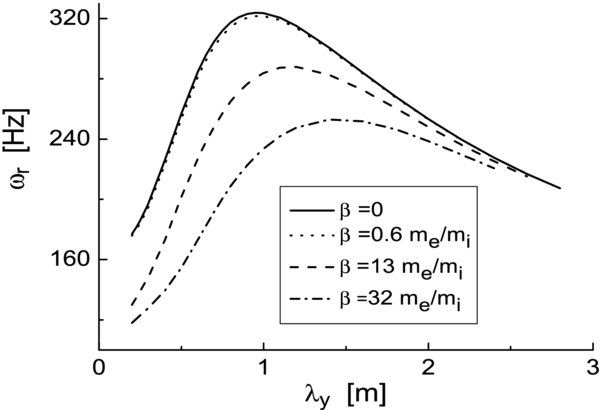
Figure 1. Drift-wave frequency for several different values of plasma β in terms of the perpendicular wavelength.
Download figure:
Standard image High-resolution imageThe plot of the growth rate corresponding to the frequencies from Figure 1 is given in Figure 2. It shows that the EM effects can make an important modification of the drift wave for larger values of the plasma-β. The reason for the reduced growth rate for short λy can be understood from Equation (14): for larger ky the coupling term on the right-hand side becomes more important, a greater amount of energy is spent on the Alfvén mode and, because of the fixed amount of the free energy stored in the background density gradient, the growth rate is therefore reduced. Hence, the physics of the stochastic heating predicted in Vranjes & Poedts (2009a, 2009b, 2009c, 2009d) will remain nearly the same even in the case of the coupling with the Alfvén mode, provided a low plasma-β. On the other hand, for a larger plasma-β the increasing EM effects will impose longer growth times.
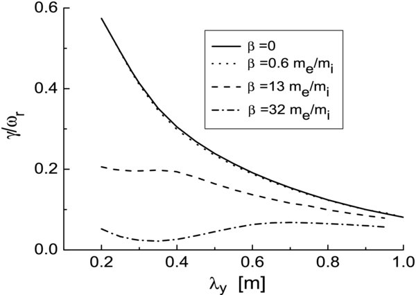
Figure 2. Normalized growth rates corresponding to the frequencies from Figure 1.
Download figure:
Standard image High-resolution imageNext, we check the drift mode behavior in terms of the parallel wavelength λz and this for several different values of the plasma-β. For that purpose Equation (12) is solved numerically and the results are presented in Figure 3 for the plasma number densities n0 = 1015 m−3, n0 = 6 × 10¹⁵ m−3, and n0 = 1016 m−3 that yield β = 0.64 me/mi, 3.8 me/mi, and 6.4 me/mi, respectively. Other parameter values are λy = 0.5 m, Ln = 1 km, and Te = Ti = 106 K. The given shape of the γ/ωr lines are equivalent to those from Figure 3 in Vranjes & Poedts (2009b). Here too, the increased EM effects reduce the growth rate. On the other hand, similar to Vranjes & Poedts (2009b), for relatively short parallel wavelength components the instability vanishes. This is due to mobile electrons which now have to move within shorter distances in the parallel direction in order to short circuit the potential buildup caused by the wave.
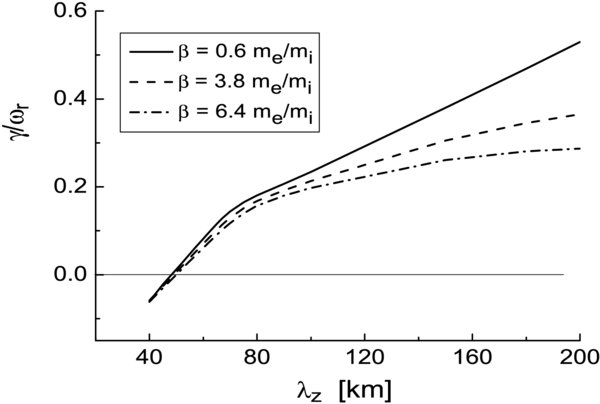
Figure 3. Normalized growth rate of the drift wave obtained from Equation (12) in terms of the parallel wavelength and for three plasma number densities n0 = 1015 m−3 (full line), n0 = 6 × 10¹⁵ m−3 (dashed line), and n0 = 1016 m−3 (dash-dotted line).
Download figure:
Standard image High-resolution imageThe plasma-β can change also by varying the temperature and/or the magnetic field. However, the drift-wave frequency is proportional to the temperature and also strongly depends on the magnetic field (see Equation (6)), so that the effect of the perturbed magnetic field alone on the drift wave in that case is not so apparent. In Figures 4 and 5, we give the drift-wave frequency and growth rate in terms of the plasma temperature for several values of the plasma density. Other parameter values are λy = 0.5 m, λz = 200 km, and Ln = 1 km. The EM effects are again most effectively seen by taking several values of the plasma density and varying the temperature. At T = 1.4 × 10⁶ K the frequency is reduced by factor of 1.4 for the density increased from n0 = 1015 m−3 to n0 = 1016 m−3. At the same time the corresponding growth rate from Figure 5 is reduced by a factor of 3.2.
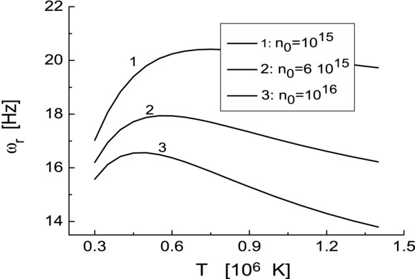
Figure 4. Drift-wave frequency obtained from Equation (12) in terms of the plasma temperature and for several values of the plasma number density (per m3).
Download figure:
Standard image High-resolution image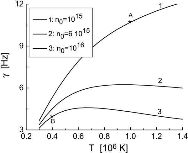
Figure 5. Drift-wave growth rate corresponding to the frequency from Figure 4.
Download figure:
Standard image High-resolution imageThe graphs presented in this section are solely for the drift-wave part of the spectrum from Equation (12). The Alfvén mode, that is also described by Equation (12), plays no important role in this study dealing with the stochastic heating. The coupling of the two modes is in fact given in detail in Vranjes & Poedts (2006) using the two-component fluid descriptions.
In view of the parameters used in this section, it is seen that the quasi-neutrality condition used in the derivations is well satisfied. This is because the Debye length λd is typically around 1 mm so that k2λ2d ≃ 0.0004 ≪ 1, and in the same time the equivalent condition Ω2i/ω2pi ≃ 0.0005 ≪ 1 is also satisfied. For these parameters, the coronal plasma from our examples is rather similar to the tokamak plasma.
6. APPLICATION TO HEATING
Considering a specific single coronal loop and in view of the given geometry that implies a very elongated wave front in the axial direction, λz ≫ λ⊥, the results presented above may imply the following. The waves propagate both axially and poloidally, with drastically different wavelength components in the two directions. In the cylindric geometry of a magnetic loop, the wave front is thus twisted along the loop. An extremely large axial component of the wavelength implies a wave that simultaneously takes place in areas with gradually varying (with altitude) plasma parameters and consequently different plasma-β. At higher altitudes with a lower density, the perturbations may be ES and develop on a shorter time scale. The associated heating may rapidly develop at such places and it can then spread along the common wave front toward lower regions where, due to the increased plasma-β, it is additionally accompanied by the EM effects that develop on longer characteristic times.
However, this scenario with an increased plasma-β due to higher plasma density can be partly counteracted by the lower temperature at lower altitudes, and as a result the energy release rate and the heating, together with the variation of magnetic topology, may not be so drastically different along the given magnetic loop. One possible example of this can be seen from Figure 5: for the given normalized temperature T = 1 from the line 1 (point A in Figure 5), the plasma-β is 0.64 me/mi, while for example at T = 0.4 from the line 3 (point B), the plasma-β is 2.5 me/mi. This is of course just a rough estimate because the points A and B belong to two separate dispersion lines. One particular plasma mode is determined by one particular dispersion line, yet in view of the parameters changing with the altitude such a transition may be expected. Hence, the drift wave spreading along the loop will have an ES nature at the first point, and it will be an EM at the second one, implying a difference in the heating rate and the magnetic variation.
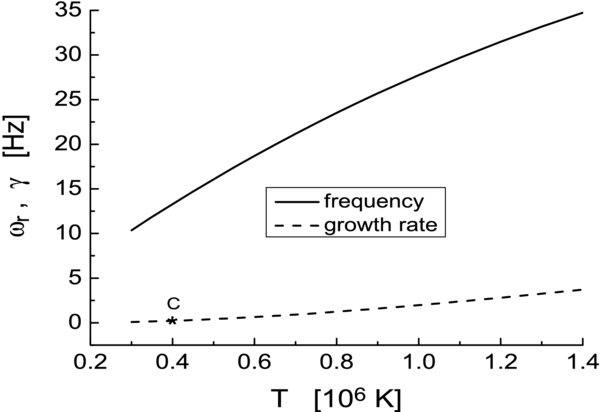
The magnetic field intensity also varies with the altitude, and this may additionally change both the plasma-β and the wave properties. Hence, assuming the magnetic field is stronger by a factor of 3 (i.e., taking B0 = 3 × 10⁻² T), and for other parameters as for line 3 from Figures 4 and 5, after solving Equation (12) again, in Figure 6 we present the wave frequency and the growth rate in terms of the temperature. Observe that, for example, at the normalized temperature T = 0.4 (the point C) the plasma-β = 0.3 me/mi, so due to the stronger magnetic field the mode is now in the ES regime (compare with the point B from Figure 5). At the same point we have the frequency and the growth rate ω = 13.3 + i0.22 Hz. Hence, for such a stronger magnetic field the growth rate becomes about 50 times lower, as compared to the ES case for the point A from Figure 5.
Figure 6. Drift-wave frequency and the growth rate for B0 = 3 × 10⁻² T; other parameters are the same as for line 3 from Figures 4 and 5.
Download figure:
Standard image High-resolution image
The points A and C in the previous examples may belong to the same magnetic loop. However, different loops may have different plasma-β and these points may also represent such a situation. Therefore, the heating in different loops may be with or without a detectable variation of the magnetic topology. Observations of strong energy release events in the past (even in the range of flares) have shown that both scenarios are indeed possible; examples without magnetic variations can be seen in Janssens (1972), Mayfield & Chapman (1981), and Pudovkin et al. (1998). The qualitative analysis described above will additionally be supported below by some more numbers.
According to McChesney et al. (1987, 1991) and Sanders et al. (1998) the stochastic heating by the drift wave is in action provided a strong enough wave potential amplitude, more precisely if
and the maximum achieved ion velocity due to this heating is given by

The effective stochastic temperature is then Tmax = miv2max/(3κ). From Equation (15) it follows that the condition for the stochastic heating will sooner be satisfied in regions of a weaker magnetic field, regardless of the starting temperature. The physics of the heating is described in McChesney et al. (1987, 1991) and Sanders et al. (1998), and its ES application to the solar corona in Vranjes & Poedts (2009a, 2009b, 2009c, 2009d), so the details of this will not be repeated here. We shall only stress that the heating is essentially due to the ion polarization drift. We shall apply these expressions using the ES and EM growth rates given above in order to quantitatively verify the differences due to eventual magnetic nature of the perturbations.
For the parameters corresponding to point A from Figure 5, Expression (15) for a = 1 yields the required potential ϕ1 = 61 V. The maximum achieved stochastic velocity from Equation (16) is 221 km s−1 and the achieved stochastic temperature is Tmax = 1.97 × 10⁶ K. Assuming some small accidental initial perturbations with the amplitude  , i.e.,
  V we can calculate the time tg required to achieve the required value for the heating
  . This yields
  s. Note also that here eϕ1/(κTi) ≃ 0.7. The total released energy density is Emax = n0miv2max/2 = 0.04 J m−3, and the energy release rate Γmax = Emax/tg = 0.1 J (m3 s)−1. Hence, Γmax is about 1700 times the required value for the coronal active regions (that amounts to ≃6 × 10⁻⁵ J (m3 s)−1 (Narain & Ulmschneider 1990)].
Taking as another example point B in Figure 5 (i.e., the same magnetic field 10−2 T but different density and starting temperature) yields Emax = 0.4 J m−3, tg = 1.3 s, and Γmax = 0.3 J (m3 s)−1, Tmax = 1.97 × 10⁶ K; β = 2.5me/mi. So, the present case is weakly EM and it is accompanied with the increase in the energy density and the energy release rate (because the density is higher), as compared to the ES case from point A, although it implies a longer growth time. The achieved stochastic temperature Tmax and velocity vmax are the same as in point A because a is kept fixed, and ϕ1 = 61 V,  V as in the previous case.
On the other hand, taking as an example point C from Figure 6, and the threshold (15), yields  V, ϕ1 = 546 V, vmax = 663 km s−1, Tmax = 1.8 × 10⁷ K, Emax = 3.67 J m−3, tg = 33 s, and Γmax = 0.11 J (m3 s)−1. The stronger necessary potential here is due to the increased value of the magnetic field, see Equation (15). Hence, the energy release rate Γmax is almost the same as for point A, yet the characteristic time tg for point A is more than 80 times shorter. In the same time, the maximum released energy density in the area with such a stronger magnetic field B0 is for about a factor of 90 larger in comparison with point A, with the achieved stochastic temperature that goes to 18 million K. The reason for the larger energy density is clearly the larger maximum stochastic velocity in the area where both the magnetic field and density are larger. The fact that plasma-β for this stronger magnetic field is only 0.3 me/mi tells us that the increased stochastic energy density can be related to the EM effects and the coupling with the Alfvén wave. However, a much more pronounced effect on the heating should be attributed to the increased magnetization of the plasma species. Thus, the areas with stronger background magnetic fields are subject to stronger stochastic heating. The magnetic field used here is in agreement with observations of active regions showing the field strength of a few times 0.01 T, that in fact may easily go above 0.1 T (Lee et al. 1998; Solanki 2003), implying a possibly still stronger heating within the scenario presented above.
Note also that the two potentials for the points A and C, 61 V and 546 V, respectively, are obtained assuming a = 1 in Equation (15). These two potentials yield the electric field kyϕ1 in the perpendicular direction 0.77 kV m−1 and 6.9 kV m−1, respectively. Now, to have the threshold a = 1, the required potential ϕ1 ∼ λyB20, so a slight increase in these two parameters will yield even stronger electric fields. Taking as an example λy = 2 m, B0 = 4 × 10⁻² (instead of λy = 0.5 m, B0 = 3 × 10⁻² as in point C) yields the perpendicular electric field at which the stochastic heating takes place Ey ≃ 27 kV m−1. The three obtained values for the electric field, together with the corresponding magnetic field values, yield the  -drift (=E/B0) of the plasma as a whole in the perpendicular direction 77, 230, and 675 km s−1, respectively. In view of the meter-sized perpendicular wavelengths these plasma flows (drifts) could eventually be observed only by spectral analysis. Hence, we conclude that (1) exceptionally strong perpendicular electric fields are expected during the proposed stochastic heating, and this particularly within stronger magnetic structures, and (2) the perpendicular stochastic heating, as a single particle interaction with the wave, is accompanied with collective plasma drifts.
7. SUMMARY AND CONCLUSIONS
The results presented in this work could be summarized as follows. The kinetic theory of the drift wave shows that the mode is almost always unstable due to purely kinetic effects and it couples naturally to the Alfvén wave. The higher the plasma-β is, the better the coupling. The ES drift wave in the solar corona is expected to be more unstable as compared to the regime in which the two modes are coupled. Essential for plasma heating is the ES part of such an EM drift-Alfvén wave. The heating is stochastic by nature and, as shown in our previous works (Vranjes & Poedts 2009a, 2009b, 2009c, 2009d), it possesses such properties that it is able to satisfy numerous heating requirements in the solar corona. From the analysis it also follows that the regions with stronger magnetic fields will be subject to much stronger heating. Note that such a relation between the temperature and the magnetic field has been established long ago (van Speybroeck et al. 1970); in this work, we give a new, alternative explanation for this phenomenon.
The electric field associated with the drift wave implies the possibility of the acceleration of plasma particles (primarily electrons) in the direction parallel to the magnetic field vector, and the development of drifts (in the perpendicular direction) of the plasma as a whole due to the  -drift that is the same for both electrons and protons. This issue is discussed in Vranjes & Poedts (2009b, 2009c). The mean free path of the plasma species j is proportional to
  and therefore the parallel acceleration by the electric field is always more effective on particles that are already faster, i.e., those from the tail in the starting (Maxwellian) distribution, because those have more time/space to interact with the field. This will consequently result in a very different distribution function with a much longer high-velocity tail and resembling the κ-distribution observed in the outer solar atmosphere. The proposed electron acceleration within the present model appears as a natural development of the drift-wave instability for which the source is clearly identified, thus removing the standard problem of various acceleration schemes that typically suffer from a common problem, the lack of a proper source.
Some phenomena that follow from the presented stochastic heating are not discussed here, but they are given in detail in Vranjes & Poedts (2009b). These include the fact that the proposed model explains the better heating of heavier particles (i.e., heavier ions are better heated than lighter ones, while the ions in general are better heated than electrons). This follows after analyzing the mass dependence of the stochastic temperature Tmax introduced earlier, with the help of Equation (16). Also the better heating in the direction perpendicular to the magnetic field vector, and the associated temperature anisotropy T⊥ > T||, is self-evident and explained in Vranjes & Poedts (2009b) as a consequence of the polarization drift that acts primarily in the perpendicular direction and becomes important at perpendicular wavelengths close to the ion gyro radius.
As stressed in Section 1, the energy for driving the instability is stored in the gradients of the background plasma. The predicted drift-wave instability will inevitably lead to the flattening of the background plasma gradients and the instability at this particular region will cease. However, the coronal magnetic structures are ever-changing and evolving, and the plasma inhomogeneity is the consequence of that. If it vanishes at one place it reappears elsewhere and the instability will reestablish itself again. The same evolving magnetic structure within which the instability and heating are developing may also simply move through the space. Such motions are observed and this all seems to be dictated by phenomena that are in much lower layers in the Sun.
Numerical simulations in the past, related to the laboratory plasma (Lee & Okuda 1976), have confirmed the mentioned flattening. However, the instability develops at much shorter time scales (the flattening is the consequence of the instability) and the heating will surely take place in such a time-evolving plasma. The previously cited experiments in tokamak plasmas support such a scenario. Similar numerical simulations with the appropriate coronal plasma parameters, aimed at supporting our analytical results, are necessary and planned.
The value of eϕ1/(κTi) in general determines the importance of nonlinearities. It turns out that in the examples discussed in the text this quantity is not small so that the presented scenario, which follows from the linear theory, may change considerably. In addition, the effects of nonlinearity in the drift-wave theory are determined also by making the ratio of the nonlinear term (i.e., the convective derivative in the momentum equation), and the leading-order linear term (Hasegawa & Sato 1989). The result can be written as (kyLn)(k2yρ2s)[eϕ1/(κT)] = kyLna. Because Ln ≫ λy, the proposed stochastic heating will be accompanied by various nonlinear phenomena. The most important nonlinear effects expected here include nonlinear three-wave interaction that implies the well-known double cascade (transfer of energy of a large amplitude drift-wave toward both longer and shorter wavelengths), and the anomalous transport caused by drift-wave turbulence. These effects, however important, require numerical simulations and will be studied elsewhere.
These results were obtained in the framework of the projects GOA/2009-009 (K. U. Leuven), G.0304.07 (FWO-Vlaanderen) and C 90347 (ESA Prodex 9). Financial support by the European Commission through the SOLAIRE Network (MTRN-CT-2006-035484) is gratefully acknowledged.