


ABSTRACT
We investigate the effect of magnetic reconnection between open and closed fields, often referred to as "interchange" reconnection, on the dynamics and topology of coronal hole boundaries. The most important and most prevalent three-dimensional topology of the interchange process is that of a small-scale bipolar magnetic field interacting with a large-scale background field. We determine the evolution of such a magnetic topology by numerical solution of the fully three-dimensional MHD equations in spherical coordinates. First, we calculate the evolution of a small-scale bipole that initially is completely inside an open field region and then is driven across a coronal hole boundary by photospheric motions. Next the reverse situation is calculated in which the bipole is initially inside the closed region and driven toward the coronal hole boundary. In both cases, we find that the stress imparted by the photospheric motions results in deformation of the separatrix surface between the closed field of the bipole and the background field, leading to rapid current sheet formation and to efficient reconnection. When the bipole is inside the open field region, the reconnection is of the interchange type in that it exchanges open and closed fields. We examine, in detail, the topology of the field as the bipole moves across the coronal hole boundary and find that the field remains well connected throughout this process. Our results, therefore, provide essential support for the quasi-steady models of the open field, because in these models the open and closed flux are assumed to remain topologically distinct as the photosphere evolves. Our results also support the uniqueness hypothesis for open field regions as postulated by Antiochos et al. On the other hand, the results argue against models in which open flux is assumed to diffusively penetrate deeply inside the closed field region under a helmet streamer. We discuss the implications of this work for coronal observations.
Export citation and abstract BibTeX RIS
1. INTRODUCTION
The solar magnetic field is the primary driver of solar activity and is the principal conduit for coupling the energy of the Sun's convective envelope to the corona and, subsequently, to the solar wind. The question of the structure and dynamics of the coronal magnetic field is, therefore, central to understanding all solar and heliospheric activity. With the advent of XUV/X-ray imaging from space missions, it became possible to observe coronal structure directly. Even the low-resolution images from the early SKYLAB mission showed clearly that the large-scale corona is composed of two physically distinct regions: "closed-field" regions, consisting primarily of bright X-ray loops, and "coronal holes" that are dark in X-rays (Zirker 1977). The photospheric flux below coronal loops is observed to be bipolar implying that the field is closed, i.e., connected to the photosphere at both ends of the coronal field lines. On the other hand, the photospheric flux below coronal holes is unipolar, on average, implying that the field there is open, i.e., connected to the photosphere at one end with the other extending outward indefinitely into the heliosphere. Coronal holes, therefore, are a source region for the solar wind, which also explains why these regions are dark in X-rays. The coronal density is low there due to the large mass and energy flux required to power the solar wind.
Motivated by the XUV/X-ray observations and by the basic theory of the solar wind given by Parker (1958), a standard model has developed for the large-scale coronal magnetic field, the "quasi-steady model" (e.g., Antiochos et al. 2007). The underlying assumptions of this model are that the magnetic field is determined by the instantaneous distribution of the large-scale radial flux at the photosphere and the balance between gas pressure and magnetic stress in the corona. In the quasi-steady model, the coronal magnetic field is assumed to be static with a smooth structure consisting of topologically well-separated open and closed regions. Of course, the flux distribution at the photosphere, even the large-scale distribution, does change with time due to flux emergence and photospheric motions; but, since typical Alfvén speeds over much of the corona are orders of magnitude greater than the driving photospheric flows, the coronal field evolution can be represented as a series of time stationary states. Note that implicit in the quasi-steady model is the assumption that flux opens and closes, most likely involving reconnection, in response to the photospheric changes.
The first and simplest implementation of the quasi-steady model was the potential field source surface model (Altschuler & Newkirk 1969; Schatten et al. 1969; Hoeksema 1991). In this model, gas pressure is neglected and the magnetic field is taken to be current-free. The open flux is determined by the assumption that the field is purely radial at some given radius (the source surface). Although the assumptions of the source surface model are extreme, it has proved to be highly useful, because it is easy to calculate and is surprisingly accurate at reproducing the observed pattern of open and closed regions on the Sun (e.g., Hoeksema 1991). Over the last decade, numerical models have been developed that calculate steady-state solution to the full MHD equations, so that the assumptions in the source surface model can be relaxed (e.g., Linker et al. 1999; Odstrcil 2003; Roussev et al. 2003). In fact, these models can even drop the quasi-steady assumption and include the photospheric time dependence, but this is rarely done due to the added complexity and computational expense. Furthermore, a rigorous time-dependent model would require robust treatment of flux emergence and cancellation, which is not yet available.
In addition to capturing the observed distribution of coronal holes on the Sun, the quasi-steady models are fairly accurate in reproducing in situ measurements of the steady solar wind magnetic field and plasma (e.g., Zurbuchen 2007; Lepri et al. 2008). Furthermore, the dynamics implicit in the model are in qualitative agreement with coronal plasma observations. The observation of plasma inflows and outflows (e.g., Hundhausen et al. 1984; Howard et al. 1985; Sheeley & Wang 2002), the observation of quasi-rigid rotation of coronal holes (Timothy et al. 1975; Zirker 1977), and the existence of the highly variable slow wind (Zurbuchen 2007, and references therein) suggest continuous opening and closing down of flux at the heliospheric current sheet, as predicted by the model.
There is one heliospheric observation, however, that appears to be in direct conflict with the quasi-steady model—the measurement of electron heat flux in the solar wind. In order to close down heliospheric flux, reconnection between two open field lines must occur at an altitude below the Alfvén point, where the magnetic energy still exceeds the thermal energy. Such a reconnection will create two loops: one having both foot points anchored to the solar surface remaining below the Alfvén point, and the other—an inverted loop—entirely detached from the Sun and dragged away with the solar wind. It is exactly this type of the reconnection process that is implied by coronal observations of the streamer belt evolution (e.g., Hundhausen et al. 1984; Howard et al. 1985; Sheeley & Wang 2002). Conversely, the opening of previously closed flux requires that a loop expand into the heliosphere and be dragged outward by the wind. It has long been recognized that such processes should produce a signature in the field-aligned suprathermal electron beams (≈70 eV to several keV) in the heliosphere (Gosling 1990). Streaming electron beams directed away from the hot corona, indicate open flux attached at a single foot point. Field lines with both foot points anchored in the solar surface and dragged into the heliosphere by the solar wind would exhibit bidirectional, counter-streaming electrons, whereas inverted loops would be devoid of these suprathermal electron beams altogether, a so-called heat flux dropout. Thus, the heat-flux electrons provide a local measure of the global field-line field topology, and as such, are a predictive indicator of flux opening and closing. The key inconsistency between heliospheric observations and the quasi-steady model is that bidirectional electron beams and heat-flux dropouts in the solar wind are rarely observed outside interplanetary coronal mass ejections (CMEs; McComas et al. 1989, 1991; Lin & Kahler 1992; Pagel et al. 2005).
Motivated by these electron observations, which imply negligible field line opening or closing, and by in situ observations implying large field line wandering in the heliosphere, Fisk and co-workers have proposed an alternative theory for the solar/heliospheric magnetic field: the "interchange model" (Fisk et al. 1999; Fisk & Schwadron 2001; Fisk 2005; Fisk & Zurbuchen 2006). In this model, the open flux is assumed to be constant during a solar cycle, except for the transient flux of CMEs. This assumption appears to be well supported by observations, which show only small variation from cycle to cycle in the total heliospheric flux at solar minimum when the effect of CMEs can be accurately removed from the heliospheric data. Note, however, that the observations for the latest minimum, cycle 23, lower the minimum heliospheric open flux threshold and may even contradict the constant-flux assumption altogether (Fisk & Zhao 2009).
The dominant process determining the open-field's evolution in the interchange model is magnetic reconnection between open and closed flux, which always conserves the amount of each type of flux (e.g., Crooker et al. 2002). It should be emphasized that the reconnection postulated by the interchange model is quite different than that in the quasi-steady model. In the latter, reconnection occurs primarily at the heliospheric current sheet, because that is where open field lines close down. Although field line opening does not require reconnection, the opening often involves the ejection of a plasmoid from the top of a streamer, which implies reconnection again at a newly formed heliospheric current sheet. Reconnection in the interchange model, on the other hand, is statistical in nature, and occurs between open flux and the closed flux of coronal loops leading to a diffusive motion of an open field in the low corona. The open field is derived to mix indiscriminately with the closed throughout the corona, so that reconnection between open and coronal-loop field occurs continuously. The interchange model, therefore, postulates a very different magnetic topology than the well-separated open and closed topology of the quasi-steady. These topological differences are a strong discriminator between the two models of the open field. For the interchange model to be valid the open-field topology must be discontinuous and inherently dynamic, whereas for the quasi-steady to hold, the topology must remain continuous throughout any coronal-field evolution.
In recent work, we analyzed the topological properties of the quasi-steady models and derived severe constraints on the possible structure of the open field. We derived, in particular, the uniqueness conjecture, which states that irrespective of the complexity of the photospheric flux distribution, every unipolar region on the photosphere can contain at most one coronal hole (Antiochos et al. 2007). Note that such a topology in which the open field has well-defined, connected structure is the exact opposite of that of the interchange model.
The validity of the uniqueness conjecture and of the quasi-steady model, in general, turns out to depend critically on the properties of interchange reconnection. The key point is that reconnection between open and closed flux is expected to be a generic feature of the solar corona and, therefore, must be incorporated into all coronal models. For example, interchange reconnection is widely believed to be a fundamental process in the magnetic reconfiguration produced by CMEs, which may be the primary mechanism by which the open field undergoes solar cycle evolution (e.g., Owens et al. 2007). Of course, explosive events such as CMEs are clearly outside the scope of the quasi-steady model, but even these global models must incorporate interchange reconnection as a fundamental feature. Due to the so-called magnetic carpet (Schrijver et al. 1997), coronal holes are obviously not unipolar; they contain numerous small bipoles and, therefore, closed flux. As these bipoles move with the photospheric flows, they will interact with the open field and undergo interchange-type reconnection. In order for the quasi-steady assumption to remain valid during such open/closed interactions, the magnetic topology must remain smooth, with the open and closed flux topologically well separated. Reconnection, however, requires the formation of current sheets, which are topological discontinuities, and reconnection generally gives rise to strong dynamics, which could invalidate the quasi-steady assumption. Consequently, it is not clear that the magnetic topology would remain smooth during actual time-dependent interchange reconnection. Our first objective in this paper, therefore, is to calculate the rigorous three-dimensional evolution of a closed field bipole as it moves through and interacts with open field and determine whether the resulting structure and dynamics are compatible with the quasi-steady assumptions or whether the topology becomes discontinuous as in the interchange model.
A related and equally important issue is the interaction of the closed field of a bipole with a coronal hole boundary. In our analysis of the quasi-steady model, we found that this type of interaction plays a central role in determining the coronal topology, including uniqueness and several other properties (Antiochos et al. 2007). We argued in that work that reconnection would allow a closed bipole field to cross a coronal hole boundary while maintaining a smooth topology as required for uniqueness, but this was only a conjecture. The second objective of this paper is to calculate the time-dependent dynamics of coronal hole boundaries rigorously and test our conjectures. We describe below our numerical simulations of three-dimensional interchange reconnection and the conclusions for coronal structure and dynamics. It should be emphasized that since the physical systems we calculate are very general and expected to be ubiquitous on the Sun, our results are important for understanding not only the quasi-steady, but any model for the coronal magnetic field, including the interchange.
2. THE TOPOLOGY OF THREE-DIMENSIONAL INTERCHANGE RECONNECTION
In order to perform a rigorous study of interchange reconnection, we first need a physically robust magnetic field. This requires a quantitative description of a complete field topology, not simply a sketch of a few open and closed field lines as used in many previous studies. The simplest and most common magnetic configuration that can describe interchange reconnection is that of a global bipolar field with open and closed regions, and a small-scale closed bipolar region. We can calculate this field exactly with an analytic source-surface model that uses the method of images (Antiochos et al. 2007). The scalar potential for the source surface field due to a global dipole at Sun center and an arbitrary number of smaller dipoles below the solar surface is given by
where Mi and ri are the magnetic dipole and position vectors respectively of dipole source i, and R is the source surface radius. Note that, for simplicity, we have taken the global dipole M0 at Sun center (x = 0) to be vertical, parallel to the polar axis, and the smaller dipoles Mi to be horizontal, perpendicular to the radius vector. Their orientation in the horizontal plane, however, can be arbitrary. From this potential, the magnetic field in the volume is obtained directly from B = grad Φ, and as can be verified by straightforward calculation, is purely radial at the source surface, r = R.
Although the formula above can be used to describe fields of arbitrary complexity, the fundamental topology of interchange reconnection is most clearly seen by focusing on the case of a global dipole and a single near-surface dipole. Such a field is shown in Figure 1, for the source surface position at R = 3 RS, a Sun-center dipole of strength |M0| = 10 G oriented toward polar north. The active-region bipole is positioned at |ri| = 0.9 RS (below the photosphere) and 49 5 latitude (i.e., north of the equator inside the northern coronal hole), with a magnitude |Mi| = 50 G oriented along the surface (i.e., with no radial component) toward the south pole. As expected, the global dipole produces a large-scale, axi-symmetric coronal magnetic field consisting of polar coronal holes and closed flux at lower latitudes (Figure 1). The near-surface dipole produces a small bipolar flux distribution that, for the particular parameters selected, is completely inside the northern, positive-polarity coronal hole. Figure 1(b) shows a closeup of the photospheric flux distribution in the hole. Note the presence of the closed polarity inversion line surrounding the negative-polarity region of the bipole. The field near this polarity inversion line is low lying and must close across it; consequently, there must be some closed flux inside the coronal hole. This is true irrespective of the size of the negative polarity region. There must be a closed field region associated with every bipole in a coronal hole.
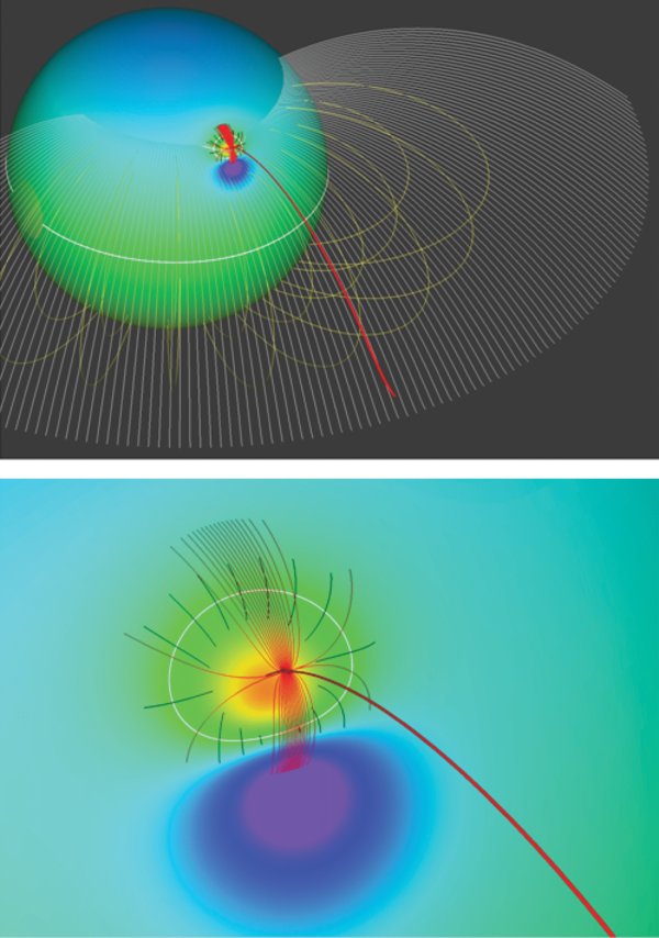
Figure 1. Magnetic topology of a small near-surface dipole and global dipole. (a) Colored contours show magnitude of the radial field at photosphere, the two white curves indicate polarity inversion lines (radial field vanishes). The yellow field lines above the surface correspond to streamer belt closed flux and the white field lines to the open, coronal hole flux that maps to the source surface. (b) Close-up of the field near the embedded bipole showing the outer fan and spine field lines.
Download figure:
Standard image High-resolution imageFigure 1(b) shows the coronal magnetic field above the small bipole. Its structure consists of a hemispherical volume of closed flux surrounded by a background of open coronal hole flux. The closed field is topologically separated from the open by a dome-shaped surface. This topology is simply that of the well-known embedded bipole with its fan surface, spine lines, and null point (e.g., Greene 1988; Lau & Finn 1990; Antiochos 1990; Priest & Titov 1996). The intersection of the fan surface with the photosphere forms a closed separatrix curve that defines the boundary between the flux that closes across the polarity inversion line to that connecting to the source surface. In other words, this photospheric separatrix curve is a coronal hole boundary. All the field lines whose photospheric footpoints lie on this curve can be considered to converge onto the null point, where they split into the inner and outer spine lines. It should be emphasized that although the topology is discontinuous at the fan and spines (i.e., the magnetic connectivity is clearly multi-valued there), the magnetic field itself is smooth everywhere. In fact, the formula above yields a potential field that is analytic everywhere in the interior of the volume. Furthermore, there is no mixing of open and closed fields. All of the flux inside the fan is closed, whereas all of the flux outside is open. The fan, itself, is a singular surface as with every coronal hole boundary in that the fan field lines split at the null, so they can be considered to both be open and closed.
The field of Figure 1 is the fundamental topology in which interchange reconnection takes place. It is, by far, the most common multi-polar magnetic topology on the Sun, because it is present whenever a parasitic polarity region on the photosphere occurs inside some larger, unipolar flux. This topology is expected for essentially every magnetic carpet, or larger, bipole on the photosphere. Numerous observations show clear evidence for this topology in coronal holes (e.g., Golub et al. 1974), and both potential and force-free extrapolations of almost every observed photospheric flux distribution find this topology in both open and closed magnetic regions (Aulanier et al. 2000; Fletcher et al. 2001; Luhmann et al. 2003).
The key question for the coronal models is whether the embedded bipole topology remains smooth, with well-separated regions, once photospheric motions stress the field so that closed and open lines interact via interchange reconnection. A rigorous answer to this question requires solution of the fully dynamic equations, as presented below, but we claim that considerable insight can be obtained by considering the heuristic model for the stressing and reconnection illustrated by Figure 2. There are two basic assumptions underlying this model. First, we can separate the ideal and resistive response of the system so that it evolves, first, purely ideally to some quasi-equilibrium, and then it relaxes by reconnection. This approach is not without justification, because reconnection will not begin until the system has formed substantial current sheets. The second assumption is that the two flux systems on either side of the fan surface move independently of each other, except that they always share a common boundary, the fan surface, which itself is free to deform. Again this assumption has justification; since the photospheric connectivity is discontinuous at the fan, the magnetic stresses due to photospheric driving will be discontinuous there, which will give rise to discontinuous motions in the corona. Note that even if viscosity were included in the system so that no true discontinuity forms, we would expect the gradients of the motions across the fan to grow exponentially in time and, consequently, the currents there to reach the dissipation scale rapidly.
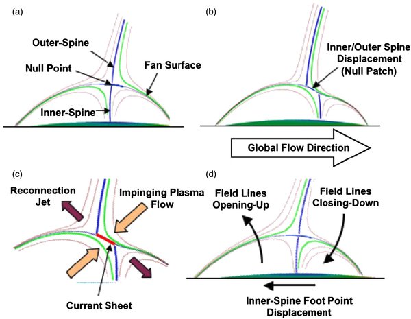
Figure 2. Interchange reconnection schematic: (a) initial field configuration; (b) stressed field configuration; (c) current sheet and reconnection jets; and (d) interchange reconnection flux exchange.
Download figure:
Standard image High-resolution imageWe can use this model to determine how the embedded-bipole topology would respond to a simple footpoint motion that displaces the closed flux system bodily to the right, while keeping the open flux more-or-less fixed (Figure 2(b)). For such a stressing, we expect that, during the ideal response, the inner spine line connecting to the parasitic polarity dislocates from the outer spine connecting to the source surface. Since each spine line "fans out" at the null to form its own surface, such a dislocation implies that the fan surface separates into two surfaces that are in contact everywhere, but with field lines that are misaligned. The effect of dislocating the spine lines and fan surfaces, therefore, is to deform the null point into a three-dimensional null patch and to form a three-dimensional current sheet at the fan. If the system were purely ideal then, in principle, it could achieve an equilibrium state containing these discontinuities.
Now let us turn on a small resistivity and consider the subsequent evolution due to reconnection. The system will attempt to relax, as much as possible, back to the potential state so as to minimize its energy. In particular, reconnection at the null-patch can destroy the current sheets and, as illustrated in Figure 2(c), deform the null patch back to a point, thereby realigning the spines, and if possible, the fans. Note that the evolution just described is nothing more than the three-dimensional generalization of Syrovatskii (1981) classic current sheet formation and null-point reconnection theory (e.g., Antiochos 1996).
The arguments above suggest that the topology resulting from reconnection will maintain clearly separated open and closed fields, as in the initial state. A key point, however, is that since reconnection conserves any helicity injected to the system by the photospheric motions, it cannot undo the photospheric motions and bring the system back to a purely potential field. In the evolution illustrated by Figure 2(c), the spine lines do not actually move, instead different flux tubes become the spines as a result of interchange reconnection. It may be, therefore, that the lowest energy state available to the system under the helicity constraints is one with long-lived (up to a dissipation time) current sheets. In fact, such a state seems inevitable if the photospheric motion is large, so that the dislocation of the spines is large. It is evident from Figure 2 that reconnection shifts the inner spine to the left by transferring closed flux from overlying the left side of the polarity inversion line to the right. The amount of flux available for such transfer, however, is limited; consequently, if the ideal motions produce too large a dislocation of the spines, reconnection will not be able to realign them.
Furthermore, there is no guarantee that reconnection will even preserve the basic spine-fan topology. Three-dimensional reconnection is likely to produce topologically complex structures so that the boundary between open and closed fields becomes chaotic and the identification of a one-dimensional spine line or a two-dimensional fan surface is no longer possible. This hypothesis seems even more likely if the closed bipole moves so that it encounters a large-scale coronal hole boundary. In that case the outer spine line would have to change from open to closed (or vice versa) and the fan would interact with the hole boundary. In order to determine the evolutionary topology and dynamics of three-dimensional interchange reconnection, we calculate numerically two simple, but highly illustrative cases. In the first case ("open-to-closed") an embedded bipole moves through an open field region and across a coronal hole boundary, into a closed field region. In the second case ("closed-to-open"), we consider the reverse situation where a bipole moves from the closed field into the open. In Section 3, we describe the numerical model—initial conditions, driving flow field, and numerical grid. Section 4 discusses in detail the simulation results for the two cases.
3. THE NUMERICAL MODEL
We solve the standard set of three-dimensional compressible, ideal MHD equations in spherical coordinates listed below, using the Adaptively Refined MHD Solver (ARMS) code (Welsch et al. 2005; DeVore & Antiochos 2008; Lynch et al. 2008, 2009; Pariat et al. 2009):
where all variables have their usual meanings. The internal energy density U is given by U = P/(γ − 1). The ratio of specific heats γ is taken to be 5/3. The ideal gas law P = 2(ρ/m) kT is used as the plasma equation of state, where k is the Boltzmann constant and m is the proton mass. Gravity, given by g = –G MS r/r3, is included in the calculations, but its effects are small with regard to the interchange reconnection dynamics. The primary reason for adding gravity is to keep the plasma beta from becoming too large at large heights.
The simulation domain consists of the spherical volume bounded below by the "photosphere" at r = 1 Rs and bounded above by the source surface, which is taken to be at r = 3 Rs. Within this domain, the initial magnetic field configuration is given by the analytic expression defined in Section 2. The origin-dipole strength |M0| = 10 G, which yields a field strength of approximately 5 G at the photosphere far from the embedded bipole. A single dipole with magnitude |Mi| = 50 G, is placed below the surface at |ri| = 0.9 Rs, the angular position of which varies between the two cases, although near the global coronal hole in both cases. Figure 3 shows the field for the case of the bipole initially in the coronal hole.
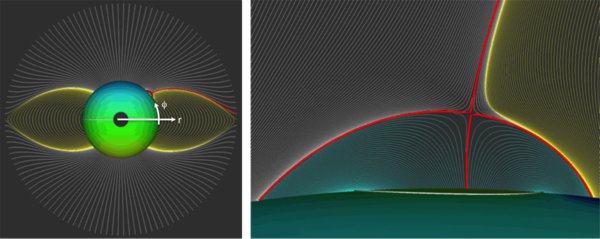
Figure 3. Global magnetic field configuration. Open field coronal hole regions are shown in white. The closed field, streamer belt region is shown in yellow. The spine and fan field lines of the embedded bipole are shown in red.
Download figure:
Standard image High-resolution imageA minor point to note is that we set the global dipole to be aligned with the y-axis (θ = π/2, ϕ = π/2) of the coordinate system rather than the vertical, as is the usual case. This implies that the coronal holes now occur centered about two points on the equator of our spherical coordinate system (at ϕ = ±π/2) rather than the coordinate poles (Figure 3). Furthermore, we select the parameters of the embedded dipole so that it is located at and oriented along the coordinate equator, and impose photospheric flows that move the resulting embedded bipolar region along this equator toward a coronal hole boundary. The reason for this choice of geometry is that the poles have metric singularities in spherical coordinates, making them difficult to treat numerically, especially in three dimensional. The simplest and most effective procedure for dealing with these singularities is to remove from the computation domain a small conical region centered about each pole, (θ < 1125 in the north and θ > 16875 in the south), visible in Figure 3 as the "holes" in the Sun. We chose the magnetic and velocity fields so that all the structure and dynamics occur at the equator, as far from these conical regions as possible. Note that there is no solar rotation in our simulation; hence, our choice of parameters for the magnetic field and flow fields corresponds only to a trivial rotation of the coordinate axis and has no physical consequences.
Since the initial magnetic field is potential, we set the initial plasma distribution to be spherically symmetric and in hydrostatic equilibrium:
where the exponent μ = R0/H0 = 11.66. The pressure scale height H0 = 2 k T0/(m g0). The surface parameters are initialized to T0 = 1 MK and P0 = 1 dyn cm−2. These plasma profiles and parameters were selected so that the plasma β would be small throughout the domain. We find that β reaches a minimum of ≈0.0325 inside the strong field of the bipole and an average value of less than ∼0.1 near the source surface; consequently, the system is low β, as in the true corona. Furthermore, the gravitational energy of the plasma is small compared to the magnetic field energy. We emphasize, however, that although the system as a whole is low β, the plasma pressure does play an important role in the evolution. Near the coronal null the plasma pressure dominates; therefore, the formation of the current sheets and the subsequent reconnection dynamics are critically dependent on the plasma evolution.
Similar to the plasma beta, the Alfvén speed varies considerably over the domain, but an average global Alfvén speed can be defined as in terms of the total magnetic energy Em and total coronal mass Mc as
With this definition, the Alfvén speed in both simulations is approximately 4 × 107 cm s−1. An Alfvén time of a little less than 115 minutes (τA ≈ 6900 s) is similarly defined using a global length scale of 4 Rs (about the length of the largest loops).
At the lower boundary, the photosphere, we impose line-tied, no-flow-through (Vr = 0) conditions. In both simulations, the embedded bipole is driven toward the coronal hole boundary by an incompressible surface flow applied at the photosphere (Figure 4). The flow field is constructed as a first-order Fourier trigonometric series in the spherical angular coordinates. The azimuthal component, Vϕ, is assumed to have cosine profiles in both co-latitude (θ) and longitude (ϕ) angular coordinates, and corresponding wave numbers that yield adjoining vortices (kθ = 1.0 and kϕ = 0.5). The polar flow component, Vθ, is then calculated by applying the vanishing divergence condition for this two-dimensional flow field,
where kt = 0.5 and tH = 1.5 × 10⁴ s = 2.17 τA. The magnitudes of these angular velocity components are set to be approximately an order of magnitude smaller than the average Alfvén speed defined above; |Vθ | = 1.875 × 106 cm s−1 = 0.047 VA, and |Vϕ| = 5 × 106 cm s−1 = 0.125 VA. Note, however, that the driving speeds above are much smaller than the Alfvén speed in the embedded bipole region, which is at least an order of magnitude larger than VA. In order to minimize transient wave effects as the motions start, the velocity magnitude has a shifted cosine profile in time. The flow is chosen to have a broad latitudinal range (θH = 0.9π, θC = 0.5π, θL = 0.1π) in order to minimize the distortion of the flux distribution within the embedded bipole as it moves across the photosphere (Figure 4).
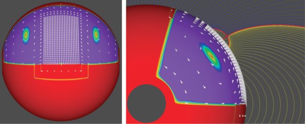
Figure 4. Surface velocity field vectors. Color scale: red indicates zero velocity magnitude; purple indicates spatial extent of flow field.
Download figure:
Standard image High-resolution imageWe use the velocity expressions above to describe the flows for both the case with the bipole initially in the coronal hole and the case with it initially in the closed field, except for a change in the longitudinal extent of the motions (and the obvious change in sign). In the first case, initially in the coronal hole, we set ϕH = 0.4π, ϕC = 0.2π, ϕL = 0.0; whereas for the second case, we set ϕH = 0.75π, ϕC = 0.375π, ϕL = 0.0. These values for the flow parameters were selected so that the bipole would definitely cross the coronal hole boundary in both cases.
At the top boundary, the source surface, we impose no-flow-through, free-slip conditions. The free slip conditions allow us to capture the physical distinction between open and closed fields without having to incorporate in the simulations the added complexity of a solar wind. The key physical difference between closed and open field lines on the Sun is that the closed lines can contain long-lived stress (electric currents), whereas the open lines must be stress-free on non-transient time scales. Since closed lines have both ends line-tied at the photosphere, they can exert a finite stress at both ends. Open field lines, on the other hand, have only one end line-tied while the other is at infinity, so that any stress injected by photospheric motions will propagate out to infinity. (Note that the other end does not have to be actually at infinity, but only out beyond the Alfvén point, which is typically at 20 solar radii, or so). We can capture this physical difference between open and closed by simply imposing free-slip conditions at the outer boundary. Field lines with both ends at the inner boundary are effectively closed, because they can hold stress indefinitely (time scales up to the dissipation time). Field lines with one end at the inner boundary and the other end at the outer are effectively open, because the free-slip condition implies that any stress injected on these lines will propagate out of the system on Alfvénic time scales. In addition to the free-slip, we impose a no-flow-through condition at the outer boundary so that we can preserve the open or closed property of a field-line under an ideal evolution. In our simulations, a field line can change from being open to closed or vice versa only as a result of reconnection and not by merely rising/sinking through the outer boundary.
Finally, Figure 5 shows the (fixed) numerical grid that is used for the simulations. The base grid consists of 64 × 96 × 192 grid points distributed uniformly in r, θ, and ϕ. In addition, we refine the grid by three factors of 2 over a sub-volume encompassing the photospheric flow field and to an altitude above the magnetic null point. The resolution at this highest refinement level corresponds to approximately 2.73 × 108 cm × 4.1 × 10−3 rad × 4.1 × 10−3 rad, which is much smaller than the scale of the embedded bipole or the flow field. Note that the grids are nearly identical for the two cases, except for minor adjustments due to the different initial position of the bipole and the latitudinal extent of the flow fields. In order to quantitatively compare the results of the two cases we have kept the grid fixed throughout the two simulations.
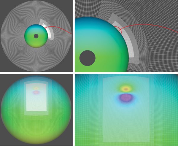
Figure 5. Numerical grid. Top panels: grid refinement in the radial direction. Bottom panels: grid refinement across the surface. Note, the initial minimum refinement is three levels above the base 2 × 3 × 6 blocks.
Download figure:
Standard image High-resolution imageThese calculations rely on numerical resistivity for the dissipation mechanism, which is most appropriate for the global problem considered here since we are trying to include as large a dynamic spatial scale range as possible. Over the majority of the coronal plasma environment the Lundquist number S is of order 1012, implying nearly ideal MHD evolution. Physically, the scales at which the frozen-in flux condition breaks down and reconnection sets in occurs at the kinetic scales such as the ion skin depth or ion gyroradius, (e.g., Cassak et al. 2005; Yamada 2007), orders of magnitude smaller than the characteristic length scales of the global model. As such, no global MHD model can accurately capture the reconnection physics. Therefore, the best that can be done is to hold the diffusion regions to occur at as small a scale as allowable. The ARMS code accomplishes this by including numerical diffusion to the ideal MHD solution whenever the current structures are localized to the grid scale. This has the effect of increasing the local effective resistivity η, or equivalently reducing the Lundquist number S. We can estimate the numerical resistivity across a given reconnection current sheet that forms as a result of global driving by balancing the inflow speed Vi of magnetic flux into the current sheet of thickness a, against the resistive annihilation across the sheet,

Solving for η,

Combining this estimate with a characteristic global scale L, such as the half-length of the spine-to-spine separation, and the local Alfvén speed VA, the effective local Lundquist number S is
Typical values for these calculations can be estimated using order of magnitude scaling. From the global average Alfvén speed and driving flow speed defined above, VA/Vi ∼ 10. The current sheet thickness is of the order of the finest resolution grid scale, a ∼ 108 cm. We assume the current sheet length L to be several high-resolution grid spaces, L ∼ 10, a ∼ 109 cm. Thus, we estimate the effective local Lundquist number S ∼ 102. Note, however, that outside the current sheet the evolution is essentially ideal, because the volumetric currents are well resolved everywhere on the grid. Thus, for example, we observe no dissipation of magnetic energy on the time scale of the simulation.
A more rigorous analysis of a time in which the current structure has developed well enough for reconnection to begin in earnest confirms this estimate. Figure 6 shows the reconnection current sheet at the fan separatrix in the open-to-closed calculation at time t = 7083.5 s. The current sheet thickness is taken to be the grid spacing in the radial direction, a = Δr = 2.73 × 108 cm. The grid spacing in the angular direction is Δϕ = 4.08 × 10⁻³ rad. The length L = 9.68 × 109 cm, is estimated using the formula, L = (Rs + nr Δr) × (nϕ Δϕ). Here Rs = 7 × 1010 cm is the solar radius; nr Δr = 15 × 2.73 × 108 cm is the altitude of the strong currents above the photosphere, where nr is the number of grid points and Δr is the grid point spacing in the radial direction; nϕ Δϕ = 4 × 4.08 × 10−3 is the angular length of the current sheet, where nϕ is the number of grid points and Δϕ is the grid point spacing in the angular direction. Averaging over the inflow speeds (and removing the rigid body motion of the global-scale dipole), Vi = 1.06 × 105 cm s−1; similarly for the outflow Alfvén speeds, we find VA = 2.48 × 106 cm s−1. Combining, we find the Lundquist number S = 1.03 × 10², in agreement with the above order of magnitude estimate. Note, as the field continues to stress, the reconnection current sheet length L will increase, which in turn will only increase the local effective Lundquist number.

Figure 6. Lundquist number analysis for t = 7083.5 s. The color contour is current magnitude |J| (red representing small |J|, and increasing to purple representing high |J|) with black contours of |J| = 5 and |J| = 10 and the full-resolution grid overlaid. From the large values of |J|, the thickness a and length L can be estimated to be 1 and 4 grid cells, respectively. The altitude of the strong |J| contours (purple vertices) are nr = 14 and 15 full-resolution grid cells from the photosphere. The white field lines represent the various flux topology domains, the spine separation is clear. The average values of Vi and VA, calculated from the vertices attached to the arrows, are quoted.
Download figure:
Standard image High-resolution image4. RESULTS
4.1. Case 1: Bipole Convection from Open to Closed Field Regions
Figure 3 shows the initial configuration for this simulation. The near-surface dipole is located at a latitude of 364, which places the outer spine inside the coronal hole, but very near the coronal hole boundary (Figure 3). We chose this initial location so that the interaction between the embedded bipole field and the coronal hole boundary would occur before extreme distortion of the closed bipole field. The evolution for the convection of the bipole from the open to closed field regions can be considered to consist of four phases.
Phase 1. From t = 0 to t ≈ 5900 s, the bipole moves toward the coronal hole boundary with evidence for only minor reconnection. Due to the finite grid of the simulation, some numerical resistivity is always present; therefore, if one examines field lines on a fine enough scale (less than the grid size), it is always possible to find some systematic flux transfer indicative of reconnection. The null point, however, remains almost undistorted during phase 1, and only weak currents (scale size substantially larger than the grid size) form there, so any reconnection is slow. The distance traveled by the inner spine during this phase is approximately 34 × 108 cm, which is a small fraction of the scale of the bipole (the diameter of the polarity inversion line in the direction of the motion is approximately 170 × 108 cm, see Figure 3). As a result of the photospheric motions, the closed field region in front of the bipole is compressed, generating stresses on the open field. These stresses displace the inner and outer spines, exactly as in Figure 2, resulting in the eventual formation of a current sheet at the deformed null.
Figure 7 presents a closeup of the null region, at t = 0, 5880, 7480, and 10,000 s. These are frames taken from a movie that is available in the electronic version of the paper. The white lines indicate initially open field lines and the yellow closed. Plotted on the vertical symmetry plane that bisects the bipole are filled contours of current density and ten black contours of β with magnitude ranging from 1 to 100. This high β region corresponds physically to the null volume where the field is susceptible to strong distortion. It is evident from Figure 7 that the deformation of the null region stays small up through t = 5800, because the β contours remain approximately circular. The currents clearly build up as the bipole's motion progresses, but at this time they are still small compared to the currents produced by the driving motions.
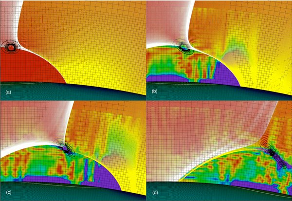
Figure 7. Open-to-closed evolution. (a) t = 0 s, initial configuration; (b) t = 5880 s, current sheet formation; (c) t = 7480 s, global topology change of external spine; (d) t = 10,000 s, final configuration.(An animation of this figure is available in the online journal.)
Download figure:
Standard image High-resolution imagePhase 2. From t ≈ 5900 s to t ≈ 7500 s the continued motion of the bipole results in sufficient deformation of the null region that the structure of the currents there decreases down to the grid scale and rapid reconnection occurs. This "interchange" reconnection exchanges the closed field of the bipole with the open field between it and the coronal hole boundary. It is most obvious in the movie, but it can also be seen in Figure 7. Note that the panel corresponding to t = 7480 has substantially fewer white field lines to the right of the closed fan surface.
We find that once interchange reconnection turns on, it stays on and smoothly moves the outer spine through the open field and closer to the coronal hole boundary. There is little evidence for explosive dynamics such as bursty reconnection or large mass outflows. The dynamics produced by the interchange reconnection in this evolution are dramatically different than those in our simulations of breakout CMEs (e.g., Lynch et al. 2008) or of coronal jets driven by magnetic twist (Pariat et al. 2009). The reason for this difference is that in the case of the CME and jet calculations, the photospheric motions are chosen so that the magnetic stress is kept away from any separatrix surface. As a result, substantial-free magnetic energy builds up inside the closed field volume until it is released by an explosive burst of reconnection, usually accompanied by some ideal instability or loss-of-equilibrium. In contrast, the large-scale translational motions of the simulation in this paper tend to move the bipole bodily, producing little magnetic stress inside its closed field. We find that only weak volumetric currents appear inside the fan and very little free energy is stored there.
The motions do produce significant stress, however, on the large-scale field where the connectivity is discontinuous, the outer fan separatrix and outer spine. This stress leads to the formation of current sheets at the fan and null region, which are quickly dissipated by reconnection without large energy release or strong impulsive behavior, at least, for the Lundquist number (S ≥ 102) of this simulation. Our result indicates that in order to obtain the large energy release to explain jets or plumes, for example, the closed field inside the fan would have to be stressed by small-scale photospheric motions as in Pariat et al. (2009) or emerge through the photosphere containing large stress. Both effects are almost certain to be true in the Sun due to the presence of subsurface convective flows and the photospheric granule and supergranule motions.
Phase 3. Interchange reconnection continues until eventually the outer spine reaches the coronal hole boundary. At some instant around t ≈ 7480 s the null of the closed field bipole lies exactly on the separatrix surface between open and closed fields and, hence, the outer spine becomes a separator line that connects the bipole null and the null at the source surface. Of course, this is a singular event. At this time the coronal hole boundary can be taken to jump discontinuously from lying in front of the bipole to behind, so that the fan bipole enters the main closed field region (Figure 7). Note that we see no evidence for any special dynamics during this period. The transition from the bipole being surrounded by the open field to closed appears smooth. This result is to be expected, because the bipole field has such small scale that its interaction with the large-scale closed field just outside the coronal hole boundary is essentially identical to that of the open field inside that boundary. As far as the magnetic field of the bipole is concerned, there is negligible difference between the open and closed field regions. Furthermore, this result agrees with observations, which indicate that, in general, no special dynamics are seen at coronal hole boundaries (Kahler & Hudson 2002).
Phase 4. During the final phase of the evolution, from t ≈ 7500 s to t = 10,000 s the bipole field moves steadily through the closed field by reconnecting with this flux. Note that although the total duration of the imposed flows is 15,000 s, we end the simulation at t = 10,000 s; consequently, the bipole is still being driven even at the end of the final phase. The reconnection during this phase is no longer of the interchange type, because it involves two closed field systems, but there appears to be little change in the dynamics. The current sheet at the deformed null region keeps increasing in length while decreasing in width (Figure 7), and the reconnection remains smooth with no apparent burstiness. We expect that if the bipole driving were to stop, the current sheet would decrease in length and the reconnection would eventually end, albeit with some residual currents left in the system.
A critical issue is the topology of the open/closed boundary throughout this four-phase evolution. The quasi-steady models require that the reconnection maintains a smooth topology with well-separated open and closed field regions (Antiochos et al. 2007). In order to determine the topology we have traced a dense sample of field lines from the source surface down to the photosphere and plotted their location there. Figure 8 shows the results for the open to closed simulation at 3 times during the simulation, and a movie showing the evolution at intermediate times is available in the electronic version of this paper.
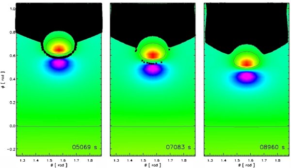
Figure 8. Open flux mapping evolution on photosphere. Open-to-closed case at t = 5069, 7083, and 8960 s.(An animation of this figure is available in the online journal.)
Download figure:
Standard image High-resolution imageThe black region in each panel is the area on the photosphere that is magnetically connected to the source surface, in other words, the open field region. Also shown are the polarity inversion lines on the photosphere (thin black lines) and filled contours of Br at the photosphere, with red indicating strong negative and blue strong positive field. We note that in the first panel, at t = 5069 s, the bipole is surrounded completely by the open field, so it is still in the coronal hole. The coronal hole forms an open corridor that extends around the negative polarity spot, but this corridor is fully connected at both ends to the main coronal hole open field region. This result shows that the mere observation of the open field in strong active region magnetic fields does not constitute evidence for the validity of the interchange model. The quasi-steady models can easily account for such observations.
As the bipole moves toward the closed field region, this open-field arch decreases in width due to interchange reconnection until by t = 7083, only a very thin corridor of open field remains (Figure 8). (The evolution is most clearly seen in the accompanying movie.) The key question is whether this corridor continues to be well connected to the main open field region or whether it breaks up into disconnected segments. It does appear from Figure 8 that the corridor has breaks, but this is an artifact produced by the finite resolution of the numerical grid and the geometry of the photospheric flux distribution. Since the negative flux is concentrated into a spot just above the strong positive flux, it is relatively easy to find field lines that connect to this negative spot. This result is also evident in the initial potential field (Figure 1). If one draws a line connecting the centers of the positive and negative spots, the fan surface has a high density of field lines in that direction but low density in the perpendicular direction, so that the fan surface appears to have gaps in this perpendicular direction. We know from the analytic expressions, however, that the fan forms a smooth continuous surface. In topological terms, the reason for these apparent gaps is that the eigenvalues of the field Jacobian evaluated at the initial null point are highly asymmetric, so that the one corresponding to the eigenvector parallel to the center-to-center line is substantially larger than the eigenvalue for the perpendicular direction (e.g., Lau & Finn 1990). This asymmetry is maintained as the spots move and, hence, the open field corridor that eventually develops also appears to have gaps. However, in Figure 9 we plot a set of field lines from the photosphere upward at t = 7083, corresponding to a time in which the open field corridor in Figure 8 appears to have large gaps. We clearly find a flux tube of open field lines completely surrounding the external spine line, separating the closed flux that connects to the negative spot from the closed flux that connects across the equatorial inversion line. Thus, the open field corridor is in fact open as shown in Figure 8 and its corresponding movie.
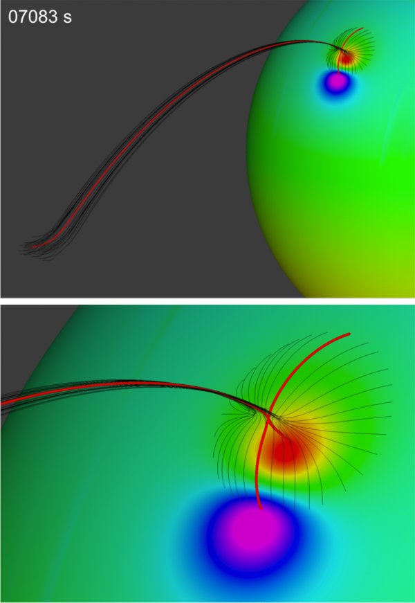
Figure 9. Field line mapping at t = 7083 s, showing an open external spine (thick red) with a set of open field lines clearly surrounding the parasitic polarity region and, thereby, proving that the open field regions of Figure 8 are fully connected.
Download figure:
Standard image High-resolution imageAs the bipole moves toward the closed field region, the open field corridor continues to thin until eventually the outer spine coincides with the open/closed field boundary, so that the corridor achieves singular width. Since our simulation has finite temporal and spatial resolution, we cannot capture this critical event when the corridor is singular. It is possible that near this time the open field corridor breaks up into discontinuous pieces, because the deformation of the null and the presence of current sheets there cause the outer spine to deform to a sheet-like structure and the fan to some fractal volume. We do not see such topologies in the simulation, the outer spine remains ray-like, but this may be due only to the finite resistivity inherent to our numerical code. Even if such singular topologies do occur, we expect that their structure would be only of order the dissipation scale and, consequently, disappear quickly. Our simulation shows only a smooth topological transition for the bipole as it moves from the open to closed regions, in good agreement with the results of the quasi-steady models (Figure 8 and accompanying movie).
4.2. Case 2: Bipole Convection from Closed to Open Field Regions
The closed-to-open case is, for the most part, closely analogous to the open-to-closed evolution. The near-surface dipole is initially located at the latitude of 360 placing the outer spine inside the closed field, very near the coronal hole boundary in order to minimize distortion during the interaction (Figure 10(a)). Again, we organize the evolution of the bipole from the closed to open field regions into four phases.

Figure 10. Closed-to-open evolution: (a) t = 0 s, initial configuration; (b) t = 3758 s, current sheet formation; (c) t = 9273 s, global topology change of external spine; (d) t = 10,000 s, final configuration.(An animation of this figure is available in the online journal.)
Download figure:
Standard image High-resolution imagePhase 1. From t = 0 to t ≈ 3758 s, the bipole moves toward the coronal hole boundary with little reconnection or current sheet formation. The distance traveled by the inner spine during this phase is approximately 80 × 108 cm, about half of the dipole polarity inversion line diameter. The photospheric motions expand the entire global closed field region, generating magnetic field stresses behind the dipole. The inner and outer spines separate as a result of these stresses, eventually deforming the null and generating a current sheet. Figure 10 shows the evolution similar to the open-to-closed case, at t = 0, 3758, 9273, and 10,000 s—movie available in the electronic version of the paper. Clearly, from Figure 10, the deformation of the null region stays small up through t ≈ 3758 s as the β contours are still approximately circular. The currents within the null region build up as the bipole motion progresses, but they are still small compared to the driving motion currents.
Phase 2. From t ≈ 3758 s to t ≈ 9273 s, the continued motion deforms the null region, decreases the current structure to the grid scale, and initiates rapid reconnection. Though not strictly interchange reconnection because the bipole is embedded in a globally closed field region, reconnection interchanges the closed flux inside the bipole fan separatrix with the large-scale closed field. Once again we find that the system evolves by continuous reconnection, smoothly shifting the outer spine through the embedding field, with little evidence of bursty reconnection or large material outflows. As above, only weak volumetric currents appear inside the fan and very little free energy is stored there.
An important difference between this case and the open-to-closed case is that the displacement required for the bipole to cross the coronal hole boundary is much larger than before. The required displacement is approximately 6.8 × 1010 cm, nearly 4 times the bipole polarity inversion line diameter. This result is due to the difference between the response of open field and closed field to photospheric stressing. Since the open field is free to slip at the source surface, significant compression stresses do not build up between the front of the bipole and the coronal hole boundary. For this case, the photospheric motions stress primarily the closed field, which is line tied at both footpoints. Consequently, the stress at the null and fan surface originates from behind the bipole as a result of the stretching of the closed field there. However, the eventual results of this stress are the same: current sheets form along the fan and deformed null region and dissipate quickly by reconnection without large energy release or strong impulsive behavior.
Phase 3. At some time around t ≈ 9273 s, reconnection between the bipole flux inside the fan surface and the external field shifts the outer spine line to the coronal hole boundary, so that the boundary jumps discontinuously across the bipole fan surface (Figure 10). Again, this singular topological transition appears smooth, showing no evidence of any special dynamics.
Phase 4. During the final phase of the evolution, from t ≈ 9273 s to t = 10,000 s the bipole field moves steadily through the coronal hole by reconnecting with the open field. The reconnection during this phase is true interchange, because the bipole is now embedded in the open field region. The current sheet aspect ratio continues to increase at the deformed null region (Figure 10), and the reconnection remains smooth. We expect that if the bipole driving were to stop, reconnection would eventually dissipate the current sheet. Since the motion is now within the open field, any helicity injected by the photospheric motions may escape the system allowing a realignment of the inner and outer spines. For this case it is possible that the system can achieve a true minimum-energy, potential state, except perhaps for any volumetric currents deep inside the closed bipole field.
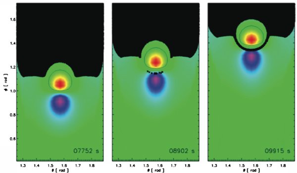
Finally, we find that the evolution of the magnetic topology (Figure 11) is essentially identical to that above. Initially, the parasitic spot is completely surrounded by closed flux. At some point near t ≈ 8902 s, the bipole is so close to the coronal hole boundary that the outer spine shifts its global topology, and a very thin open field corridor forms. The open field corridor is well connected to the main coronal hole even though in the figure it appears to have breaks; the same arguments as in the open-to-closed case apply. Once the motion is completely inside the open field coronal hole, the corridor continues to thicken as flux is transferred across the bipole fan surface (Figure 11). The sequence shown in Figure 11, therefore, is simply the reverse of that in Figure 8.
Figure 11. Open flux mapping evolution on photosphere. Closed-to-open case at t = 7752, 8902, and 9915 s.(An animation of this figure is available in the online journal.)
Download figure:
Standard image High-resolution image
5. CONCLUSIONS
The results described above have a number of implications for understanding the corona/heliosphere and interpreting observations. The first and, perhaps, most important conclusion is that the basic topology of the interchange process is that of the closed field of a bipole interacting with surrounding open field, as in Figure 2. The reconnection occurs at the fan surface, primarily at the null. Note that the topology is continuous and, hence, it is not valid physically to assume a picture in which reconnection takes place between an isolated open and closed field line. The difference between the continuous topology of Figure 2 and the often-used discontinuous picture may seem minor, because in both models the open field undergoes a jump in the footpoint position as a result of reconnection. The key point, however, is that in the continuous model the reconnection releases energy only after a large current sheet forms. If the reconnection at the null is highly efficient, the open field will smoothly transfer from one side of the bipole to the other with no heating or mass acceleration. Even though copious interchange reconnection may be present in coronal holes, this reconnection can play a significant role in the heating and acceleration of the wind only if intense current sheets are present, as well. We conclude, therefore, that an accurate treatment of the reconnection, especially of the effective resistivity, is required in order to evaluate the importance of the interchange process to the formation of the solar wind.
From our simulations, we find that the magnetic topology remains smooth throughout the interchange reconnection process, even when a bipole crosses a helmet streamer boundary. Our results, therefore, constitute strong support for the quasi-steady models in which the large-scale field evolution can be approximated as a sequence of topologically smooth quasi-steady states. One aspect of this general result is that the uniqueness conjecture (Antiochos et al. 2007) appears to hold even during interchange reconnection. We see no evidence for disconnected coronal holes as the bipole evolves. It could be argued that we have calculated the evolution of only a single bipole moving in a simple trajectory and that our results may change for a system with the complexity of the true solar field. This complexity, however, is simply that of a superposition of many bipoles. We expect that for such a field the instantaneous topology would remain well connected, as in Figures 7 and 9, but with many more open-field corridors. This is exactly the topology that we obtained using the source surface model with high-resolution solar observations (Antiochos et al. 2007).
Our result that the open field remains well connected argues against the basic assumptions of the interchange model. On the other hand, if a sufficiently complex distribution of bipoles is present, then certain features of the interchange model, such as open-flux diffusion, start to become valid. The interchange model of Fisk et al. (1999) assumes that the evolution of the open field is dominated by its random reconnections with a dynamic complex of closed loops. Although the magnetic topology invoked by the interchange model is not supported by our results, the simulations show that when the bipole is inside the open field region, interchange reconnection readily occurs and it does, indeed, cause open flux to jump from one side of the bipole to the other. If enough bipoles are present, this evolution of the open flux may well be best described as a diffusion process. Note, however, that this diffusion occurs only inside the open field region. The reconnection does not allow the open flux to penetrate into the closed field regions.
Another important result from the simulations is that unlike the source-surface model, the field does not remain current-free during the evolution. Large currents form in the corona in response to the photospheric motions, and these currents are long-lived. Consequently, the exact position and geometry of the open/closed boundary will be different than that calculated from the source surface model, which is important for comparison with observations, but the model should still be qualitatively correct. Given the proper boundary conditions, the MHD models can, in principle, calculate the field and currents precisely, but determining such boundary conditions from available observations may not be possible.
From the viewpoint of comparison with observations, a key result from our work is that the reconnection does not produce bursty dynamics. Energy is released during the reconnection, primarily as mass flows, but the release does not show the type of impulsive behavior that we have seen in previous simulations of coronal reconnection (e.g., Karpen et al. 1998; Pariat et al. 2009). There are several possible reasons for this difference. First, the photospheric driving in the present simulations does not impart significant shear or twist to the field, unlike the case of our coronal jet model (Pariat et al. 2009). Consequently, the energy released by the interchange reconnection is only the energy in the local current sheet at the null region, not the free energy of currents in a large volume. Second, the reconnection is fully three dimensional, which makes it more difficult for magnetic islands to form. In our 2.5D simulations (Karpen et al. 1998), we found that much of the burstiness was due to the random formation and expulsion of magnetic islands in the reconnecting current sheet. Another problem is that, even with adaptive mesh refinement, the three-dimensional calculations simply have less numerical resolution that the 2.5D runs, so that the effective diffusion is larger. The runs discussed in this paper required hundreds of thousands of processor hours with a highly optimized code and, therefore, represent the present state of the art. It is possible that, eventually, three-dimensional runs will have sufficient numerical resolution to produce current sheets with very large aspect ratios and, consequently, reconnection dynamics resembling more closely those of the 2.5D results.
On the other hand, observations of bipoles in coronal holes do not appear to show strong dynamics, which suggests that our results above may hold even in the limit of large Lundquist number. Coronal jets are relatively rare events. In most cases embedded bipoles are associated with long-lived plumes, which require a quasi-steady heating (e.g., Wang & Muglach 2008). The type of reconnection that we obtain in the simulations above would be compatible with this type of heating. It is difficult, however, to compare our results quantitatively with plume observations, because we do not include a proper treatment of the plasma energetics. Our initial conditions assume a spherically symmetric density distribution, but on the Sun, the densities inside the closed field region of a coronal hole bipole are clearly much larger than the density of the surrounding open field. Interchange reconnection between the closed and open field will release this high-density (and pressure) material onto open field lines, which would then expand outward and, perhaps, form a plume. Further calculations with more realistic plasma energetics, including radiation and thermal conduction are needed in order to test such a model.
It is tempting to conjecture that this process of releasing the closed-field plasma of embedded bipoles onto an open field is also the origin of the slow wind, because in situ measurements have shown that the slow wind has the distinct compositional signature of closed-field plasma (e.g., von Steiger et al. 2000; Zurbuchen et al. 2002). The problem with this conjecture, however, is that closed bipoles are observed to occur throughout coronal holes. Consequently, if the release of embedded bipole plasma were the source of the slow wind, this wind would be observed from the middle of coronal holes, far from the heliospheric current sheet. The fact that slow wind is seen only near the current sheet, within 15° or so, implies that the origin of the slow wind must be associated with coronal hole boundaries, and not with the interchange reconnection due to the magnetic carpet.
Although the interchange reconnection in our simulations is unlikely to be the primary source of the slow wind, we conjecture that some of the topological features may well play a key role. We note from Figures 7 and 9 that when a bipole moves through a coronal hole boundary, narrow open field corridors appear and disappear. If there are many bipoles moving randomly in response to photospheric motions, the coronal hole boundary will consist of a complex dynamic web of open-field corridors, which as suggested previously, may be the source of slow wind (Antiochos et al. 2007). It is interesting to note that such a complex web of open field corridors could blur the distinction between the interchange and quasi-steady models, but only in the vicinity of coronal hole boundaries. The quasi-steady models, and our simulations, are fully deterministic in that given the flux distribution at the photosphere, the open and closed regions are completely determined by the MHD equations. In principle, this result holds irrespective of the number of bipoles and the resulting complexity of the open/closed boundary. But if sufficiently complex, it is likely that the only tractable procedure for calculating the dynamics of the open/closed boundary region would be to develop a statistical treatment in the spirit of the interchange model. We propose that a mixing of the two approaches, deterministic and statistical, may well be the key to understanding the origins of the slow wind.
This work was supported, in part, by the NASA HTP, TR&T, and SR&T Programs, and has benefited greatly from the authors' participation in the NASA TR&T focused science team on the solar-heliospheric magnetic field. All the high performance computing capabilities were provided by the DoD HPCMP. J.K.E. gratefully acknowledges support of a NASA GSRP grant for his PhD research.