ABSTRACT
We extend the analysis of Penev et al. to calculate effective viscosities for the surface convective zones of three main-sequence stars of 0.775 M☉, 0.85 M☉, and the present day Sun. In addition, we also pay careful attention to all normalization factors and assumptions in order to derive actual numerical prescriptions for the effective viscosity as a function of the period and direction of the external shear. Our results are applicable for periods that are too long to correspond to eddies that fall within the inertial subrange of Kolmogorov scaling, but no larger than the convective turnover time, when the assumptions of the calculation break down. We find moderately anisotropic viscosity, scaling linearly with the period of the external perturbation, with its components having magnitudes between three and ten times smaller than the Zahn's prescription.
Export citation and abstract BibTeX RIS
1. INTRODUCTION
Turbulent (eddy) viscosity is often considered to be the main mechanism responsible for the dissipation of tides and oscillations in convection zones of cool stars and planets (Goodman & Oh 1997, from now on GO; and references therein). Currently existing descriptions have been used, with varying success, to explain circularization cutoff periods for main-sequence binary stars (Zahn & Bouchet 1989; Meibom & Mathieu 2005), the red edge of the Cepheid instability strip (Gonczi 1982), and damping of solar oscillations (Goldreich & Keeley 1977). However, this hypothesis has been far more successful in damping oscillations than damping tides, and different mechanisms have been proposed for the latter, especially for planets (see Wu 2005a, 2005b; Ogilvie & Lin 2004 and references therein).
The standard treatment is to assume a Kolmogorov spectrum in the convection zone and apply some prescription to model the effectiveness of eddies in dissipating the given perturbation. Two prescriptions have been proposed to describe the efficiency of eddies in dissipating perturbations with periods (T) smaller than the eddy turnover time (τ).
The first prescription, due to Zahn (1966, 1989), assumes that it is always the largest eddies that dominate the dissipation and that they lose efficiency linearly with decreasing period:

where νmax is some constant which depends on the mixing length parameter and τc is the local convective turnover time (or the turnover time of the largest local eddies). This prescription has been tested against tidal circularization times for binaries containing a giant star (Verbunt & Phinney 1995), and is, in general, in agreement with observations.
The second prescription, due to Goldreich & Nicholson (1977) and Goldreich & Keeley (1977), assumes that eddies with periods longer than T/2π do not contribute to the dissipation. In that case, for Kolmogorov scaling:

This prescription has been used successfully by Goldreich & Keeley (1977); Goldreich & Kumar (1988); and Goldreich et al. (1994) to develop a theory for the damping of the solar p-modes. If the more effective dissipation was applied instead, dramatic changes would be required in the excitation mechanism in order to explain the observed p-mode amplitudes. However, this inefficient dissipation is inconsistent with observed tidal circularization for binary stars (Meibom & Mathieu 2005). Additionally, Gonczi (1982) argues that for pulsating stars the location of the red edge of the instability strip is more consistent with Zahn's description of the eddy viscosity than with that of Goldreich and collaborators.
GO gave a consistent hydrostatic derivation of the convective viscosity, using a perturbation approach. For a Kolmogorov scaling, they obtained a result that is closer to the less-efficient Goldreich & Nicholson viscosity than it is to Zahn's, providing a more sound theoretical basis for the former scaling. Of course, the observational problem of insufficient tidal dissipation for stellar pulsations and binaries remains unresolved, as GO point out.
Both two-dimensional (2D) and three-dimensional (3D) numerical simulations of the solar convection zone have revealed that the picture of a Kolmogorov spectrum of eddies is too simplified (Stein & Nordlund 1989; Robinson et al. 2003). These simulations show that convection proceeds in a rather different, highly asymmetric fashion. This suggests that the problem of insufficient dissipation may be resolved by replacing the assumption of Kolmogorov turbulence with the velocity field produced from numerical simulations. More importantly, an asymmetric and non-Kolmogorov turbulence might dissipate different perturbations differently, i.e., depending both on the frequency and geometry of the perturbation. Such simulations have been used to develop a better model for the excitation of solar p-modes (Samadi et al. 2003).
In Penev et al. (2007), we reconsidered the problem of tidal dissipation in stellar convection zones of solar-type stars by applying the approximation developed in GO to the turbulent velocity field from a realistic 3D solar simulation and showed that the scaling predicted by this procedure is very close to linear. The shallower scaling is explained by the fact that on the timescales captured by the simulation the largest eddies have typical sizes comparable to the local pressure scale height and, in this regime, the velocity power spectrum is much shallower than Kolmogorov.
In this paper, we apply a more complete version of the same scheme to three stellar convection models appropriate for stars with masses of 0.775 M☉, 0.85 M☉, and 1 M☉. We also pay significantly more attention to the normalization and the approximations which we introduce in addition to GO.
2. METHOD
2.1. The Perturbative Expansion for Discretely Sampled Velocity Field
We follow the procedure outlined in GO and assume an external perturbing velocity field given by GO's Equation (8):

where A(t) is some matrix that depends only on time, and not space. This is appropriate when the spatial dependence of the perturbation is on scales much larger than our simulation box (e.g., tides). The matrix A(t) is assumed symmetric, since the antisymmetric part corresponds to rotation, and is not expected to contribute to the energy dissipation.
Introducing this velocity field will modify the convective flow (v0). The time evolution of the change in the turbulent velocity (δv) due to the presence of the above external field can be written as in GO, Equation (19):

GO assumed incompressibility, and hence the pressure term simply maintains that ∇ · δv = 0. We use the output of fully compressible simulations, so for us the pressure term should be much more complex. However, the only type of compressibility that we can reasonably incorporate in the analysis is that due to the stratification of the convective layer, and even that we approximate by assuming a constant density scale height. This is discussed in more detail in Section 2.3.
We then follow GO in writing Equation (4) in Fourier space. However, since we are dealing with discretely sampled data, we use discrete Fourier transforms:
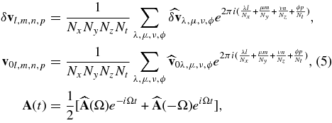
where 2π/Ω is the period of the external forcing.
For more details on how exactly the Fourier transform is applied in the radial and time directions see Section 2.4.
In Fourier space to first order in A (the strength of the perturbation) and Ωτc (the ratio of perturbation timescale to convective turnover time), Equation (4) is written as

where Pλ,μ,ν ≡ I − k'λ,μ,νk'λ,μ,ν/k'2λ,μ,ν, with  , is the discrete version of the projection operator GO defined that imposes compressibility only due to a constant density scale height.
We can then express the average rate of work done (per unit volume) on the turbulent velocities by the tide to lowest non-zero order as
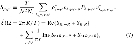
where  . In keeping with GO, we have assumed that all frequencies have an infinitesimal imaginary part, which gives rise to the first term above. The second term is entirely due to the density stratification in the box: in the case of
  , it is zero. This term is the most important difference between this calculation and GO.
In deriving Equation (7), we have assumed that the density is only a function of depth. Keeping the radial dependence is necessary because the simulation box encompasses several density scale heights, while the horizontal and temporal dependence of the density is a much smaller effect, entirely due to the turbulent fluctuations in the box; and if we could average over different realizations of the turbulence, they would not be present.
2.2. Anisotropic Viscosity
In order to extract an effective viscosity, we need to express the energy dissipation rate that would occur in the presence of actual anisotropic viscosity.
Most generally, viscosity is a fourth-order tensor relating the strain, given by A(t) in this case, and the viscous stress:

With this definition the time-averaged dissipated power is given by:

where, in order to remain consistent with the Fourier transform conventions, we simply replace the integral with a sum. To get the different components of Kijmn, we evaluate Equation (7) with A having non-zero elements at different locations, and use the above equation to find the respective viscosity coefficients.
The viscosity tensor (Kijmn) obeys a set of symmetries that dramatically reduce the number of independent components. Since the strain rate is symmetric by definition, and the stress must be symmetric in order to keep the viscous torque on infinitesimal fluid elements finite, we must have

In addition, the only distinct direction in the problem is that of gravity ( ), so we expect the viscosity tensor to be symmetric with respect to rotation around the vertical axis.
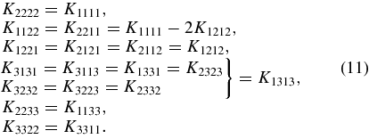
With all these symmetries we are left with only six independent components of Kijmn: K1111, K3333, K1212, K1313, K1133, and K3311. Since the last two of these always appear together in the expression, for the energy dissipation we will assume them to be equal. The remaining non-zero components can be found from those as follows:
A more physically meaningful set of five viscosity components can be found by noting that under these symmetries the strain rate has only four distinct components:

along with their complex conjugates  , which transform under rotation by angle θ around the
  -axis as
  .
.
Clearly then, if  is to be invariant under such rotations, it must be of the form:

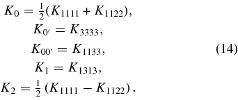
where the five new viscosity coefficients can be expressed in terms of Kijmn as follows:
Since in Equation (9), we allow the viscosity to depend on depth, and there is no way to constrain this dependence, we have to choose some radial profile a priori. Our choice is motivated by mixing length theory:

where K0m are dimensionless constants that depend on the frequency of the external shear (Ω), and Hp is the local pressure scale height. This is reasonable, since the turbulent viscosity should scale as some length scale times some velocity scale. Clearly the relevant velocity scale is that of convection, and in accordance with mixing length theory, we use the mixing length as the length scale, which is assumed proportional to the pressure scale height. If the mixing length is really the relevant quantity, we expect that the value of K0m will be proportional to the mixing length parameter for the particular simulation. This same scaling has been assumed for all previous effective viscosity prescriptions (Zahn 1966, 1989; Goldreich & Keeley 1977; Goldreich & Kumar 1988; Goldreich et al. 1994).
2.3. The Pressure Term
In deriving the expression for  (Equation (7)), we assumed that the perturbation to the convective velocity field due to the tide will be anelastic: ∇ · δv + vz/Hρ = 0, with
  . In this section, we define two diagnostics which measure how important the ignored compressibility is.
There are two sources of compressibility in the convective flow:
- 1.The convective flow carrying parcels of matter through layers of different hydrostatic pressure, or in other words due to the stratification.
- 2.Localized compression due to a possibly supersonic flow, e.g., shocks.
Ignoring the second one is justified, as long as the flow velocity is much less than the local speed of sound. In the simulations we use, that condition is met by the unperturbed flow for most of the box, with the exception of the supersonic driving region near the top. If the unperturbed flow is subsonic and hence incompressible, the perturbations due to a "small" external field can safely be assumed incompressible as well. To measure the compressibility in the simulation box, we introduce the parameter:

where, ρ is the density averaged over horizontal slices and time.
This quantity deviates from zero due to localized, transient compressions (e.g., shocks). Since those are unlikely to live longer than a convective turnover time, this quantity is a suitable diagnostic for the importance of such effects.
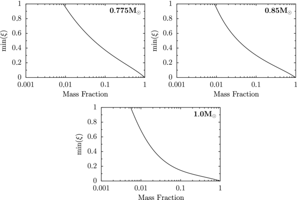
Because we are measuring the mass-averaged dissipation, in order for the perturbative treatment discussed above to be valid, we can only have ξ ≳ 1 for a negligible fraction of the mass. In Figure 1, we plot the time-averaged fraction of mass that resides in regions of the convective box which have ξ greater than some value. The value of the convective turnover time, necessary to evaluate ξ, was calculated as τc ≡ FWHM(vz)/max(vz), where FWHM(vz) is the thickness of the layer over which vz>max(vz)/2.
Figure 1. Compressibility of the unperturbed flow as a function of depth for the three simulation boxes (0.775 M☉—top left; 0.85 M☉—top right; and 1.0 M☉—bottom). The horizontal axis gives the time-averaged fraction of mass with compressibility greater than the vertical value.
Download figure:
Standard image High-resolution imageAs we can see, in all cases, ξ>1 for less than 1% of the mass. This compression is concentrated near the top of the box, where the density, and hence the dynamic viscosity, is small. So, even though compressibility and shocks are important in determining the flow that develops, no appreciable dissipation occurs in strongly compressible regions. The situation is further improved by the fact that we apply a window in the vertical direction that significantly reduces the importance, and completely ignores part of the compressible driving region near the top of the box in determining the effective viscosity (see Section 2.4).
We partially treat the first source of compressibility discussed above by, imposing  in the continuity equation. However, this is not valid for most astrophysically interesting convective zones. In fact in all cases considered here the density scale height varies by a factor of a few between the top and the bottom of the convective layer. In some sense, assuming
  is not any better than assuming Hρ = ∞. We argue that ignoring the stratification from the continuity equation is a reasonable approximation.
The simplest way to justify this is to repeat the evaluation of the viscosity with different values of Hρ within the range encountered in the convective layer of interest.
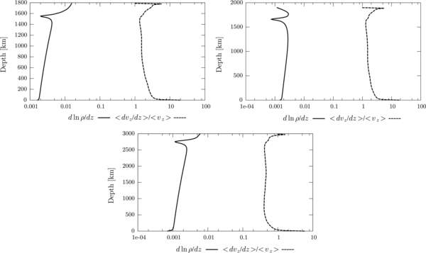
We can also gauge the importance of the stratification by comparing dln ρ/dz to ∂ln δvz/∂z. We evaluate dln ρ/dz directly, and estimate:

The last expression comes from Equation (6), and is correct when the last row of A(t) contains only a single non-zero entry. Since those are the only cases we use, this expression is sufficient for us.
In Figure 2, we compare dln ρ/dz to ∂ln δvz/∂z (estimated as in the above expressions). We see that the logarithmic gradient of the density is approximately 2 orders of magnitude smaller than the typical logarithmic velocity gradient, and hence we are justified in ignoring it.
Figure 2. Logarithmic gradient of the density compared to the logarithmic gradient of vz, estimated as explained in the text for the three simulation boxes we considered: 0.775 M☉—top left; 0.85 M☉—top right; and 1.0 M☉—bottom.
Download figure:
Standard image High-resolution image2.4. Radial and Time Fourier Transforms
Using discrete Fourier transforms to represent a data set, forces the assumption that the data is periodic in all dimensions. While this holds for each horizontal slice, it is violated for the radial and time dimensions. Ignoring the problem leads to artificially introducing spectral power at the highest frequencies because of the jumps at the boundaries. To avoid this, we need a special way to deal with the non-periodic directions.
The usual solution is to window the data so that it goes smoothly to zero at the edges of the domain. This has the effect that it makes the values near the center of the domain relatively more important than those near the boundaries. Incidentally, this is exactly what we would like in the radial direction, since the flow near the top and the bottom is affected by the artificial boundary conditions and is not representative of the actual flow that would occur in a star.
Further, as discussed in Section 2.3, we expect that the compressibility of the flow that we neglect might be significant in the upper end of the box, where the density is small and the flow is supersonic. So making this region's contribution to the overall dissipation small is exactly what we would like. In fact, in the radial direction we go a step further and limit the window to completely exclude some part of the box near the top and bottom boundaries (see Equations (18) and (19)).
In the time direction, as long as the time interval we have simulated is "representative" of the actual convection that occurs in a star, weighing the center of the interval more than the edges should not be a problem.
To confirm that the chosen window function is not affecting our final result, we derive the effective viscosity coefficient using two common windows:


where  is a normalization factor numerically equal to the inverse of the average of the squares of the window function at all the grid points, and α is a parameter determining what fraction of the radial span of the box we include in the analysis; that is, we exclude (1 − α) fraction of the linear size of the box, half from the top and half from the bottom.
3. THE STELLAR MODELS
The three models used, represent the top 7–9 pressure scale heights of the convective zones of the present Sun, a 0.775 M☉ and a 0.85 M☉ stars. Table 1 shows the position of each model in the log g − log Teff plane. The full details of the numerical scheme and the properties of the solar simulation are discussed in Robinson et al. (2003). For a comparison between the models used here and the work of other groups, as well as observations see Kupka (2005) and Hillebrandt & Kupka (2009). Here, we present very briefly only the most important aspects of the models.
Table 1. The Physical Characteristics of the Three Simulations Used to Derive Effective Viscosities
| Model Mass | 1 M☉ | 0.85 M☉ | 0.775 M☉ |
|---|---|---|---|
| Age (Gyr) | 4.55 | 7 | 2 |
| log Teff | 3.761 | 3.685 | 3.708 |
| log g | 4.44 | 4.592 | 4.592 |
| R/R☉ | 1.0 | 0.737 | 0.772 |
| Size (Mm) (Lx × Ly × Lz) | 5.42 × 2.8 | 2.72 × 1.8 | 2.92 × 1.9 |
| Grid (Nx × Ny × Nz) | 1142 × 170 | 1152 × 170 | 1152 × 170 |
Note. The units of Teff are K, and the units of g are cm s−2.
Download table as: ASCIITypeset image
The simulation boxes have periodic sidewalls and impenetrable top and bottom surfaces with a constant energy flux fed into the base and a perfectly conducting top boundary. The imposed flux was computed from a corresponding one-dimensional (1D) stellar model with the chosen mass and age, thus was not arbitrary, but the correct amount of energy flux the computational domain should transport outward in the particular star. The initial conditions of the 3D simulations were also derived from the same 1D stellar models used to calculate the required flux.
3.1. Starting Models and Input Physics
The 1D stellar models used to initialize each run were computed with the YREC stellar evolution code (Guenther et al. 1992). They were calibrated to the Sun and evolved from the ZAMS. Both the 1D and 3D codes use the same realistic physics as described by Guenther & Demarque (1997), most notably the Alexander & Ferguson (1994) opacities at low temperatures, the OPAL opacities and equation of state (Iglesias & Rogers 1996), hydrogen and helium ionization and helium and heavy element diffusion.
Some details of the three models are given in Table 1. The fractional radius is given as R/R☉, where R is radius of the stellar body and R☉ is the radius of the Sun. Both are defined at the point where T = Teff. The surface gravity and effective temperature are in cgs units.
3.2. Box Dimensions
The horizontal dimensions of each computational box (Row 5 in Table 1) were estimated by assuming that the granule size will roughly scale inversely with g. The final row gives the number of grid points in the two horizontal and vertical directions in the square based box.
4. RESULTS
As discussed in Section 2.2, the anisotropic viscosity can be parameterized by five independent components. Assuming Equation (15), we evaluate those components using the two window functions of Equations (18) and (19) each with two different values of α: 0.8 and 0.9. In addition, we use two values for the density scale height in each case: Hρ = ∞ and the volume average density scale height.
The reason for using the volume-averaged value of Hρ instead of the mass-averaged is that, this way, relatively more weight is given to the less-dense top regions where the density scale height is small, resulting in a larger range between the two cases we consider.
The frequency dependence of the five viscosity coefficients (K0,  ,
,  , K1, and K2) is presented in Figure 3, the curves correspond to a Welch window (Equation (18)) with α = 0.9; and volume-averaged density scale height and the error bars show the span among all the cases for which we evaluated the effective viscosity.
Figure 3. Five viscosity components, scaled by 〈v2〉1/2Hp for the three stellar models (0.775 M☉—top left; 0.85 M☉—top right; and 1 M☉—bottom). The lines correspond to the average of all curves representing the same component calculated using α = 0.9, Welch window (Equation (18)) and the volume-averaged density scale height. The error bars correspond to the spread found among all the curves corresponding to the viscosity component with different windows, values of alpha and density scale heights.
Download figure:
Standard image High-resolution imageThe fact that the error bars in Figure 3 are small shows that indeed the choice of the window function is not important and that ignoring the depth dependence of the density scale height, and in fact the stratification altogether in the continuity equation is a valid approximation.
We see that the same qualitative characteristics hold for the estimated dissipation in all three of our simulation boxes: the  component is always approximately four times larger than the K0, K1, and K2 components, which are in turn roughly four to five times larger than the
  component and the scaling is approximately the same for all components, close to the linear scaling proposed by Zahn.
Quantitatively, the effective viscosity we calculate can be written as

where the parameters  and λ take the values:
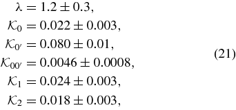
with the errors corresponding to the range of values encountered for different windows, values of α, density scale heights, and stellar models. The above values were derived by performing a least squares fit of Equation (20) to the calculated curves for T < 0.5τc. The reason for restricting the fit to short periods is that at long periods we do not expect the perturbative calculation used in this work to be applicable, and hence the derived slope is an artifact of the model rather than having any physical significance.
Also there is no appreciable difference between the models of the different stars. The spread in the dimensionless effective viscosities for the three models is not much larger than the error bars at all frequencies, except the high end tails, where the effects of the finite resolution and time sampling become important. This suggests that at least for the range of conditions encountered in the convective zones of low-mass stars, the dissipation efficiency is not strongly dependent on the details of the convective flow.
4.1. Anisotropy
The above splitting of the viscosity in five components was done in order to allow for anisotropic dissipation. It is interesting to see how anisotropic the derived effective viscosity really is. The general isotropic case has only two viscosity components: a bulk viscosity (ζ) and a shear viscosity (η) (see Landau & Lifshitz 1987). In terms of these components, the isotropic Kijmn tensor is

From this it can be seen that the five components of the viscosity we calculate must obey the relations:

We see that the first two of these are clearly satisfied by the viscosity coefficients of Equation (21) to within the quoted uncertainties. The degree to which the last equation is not satisfied is

Considering the fact that the flows in our simulation boxes are not exactly like those inside the stars, and the loosely estimated errors in Equation (21); we can conclude that the effective viscosity we find is only mildly anisotropic, and it is perhaps reasonable to approximate it as completely isotropic bulk and shear viscosities with the following values:

The reason for ζ not being well determined by the viscosity coefficients of Equation (21) is that those coefficients do not exactly correspond to an isotropic viscosity (see Equation (24)).
5. CONCLUSION
We have extended the analysis of Penev et al. (2007) to calculate effective viscosities in the surface convective zones of three main-sequence stars: 0.775 M☉, 0.85 M☉, and the present day Sun. We have also modified the calculation to properly account for all normalization factors.
The effective viscosity we find (given by Equations (20) and (21)) scales linearly with the period of the external perturbation, with the shear viscosity being smaller than the linear scaling proposed by Zahn (1966, 1989) by a factor of about 10, but in addition there is a significant bulk viscosity, which is assumed zero in Zahn's prescription.
This factor, in practice, does not have a dramatic effect on the tidal circularization period, which scales as K3/16 (Zahn 1966, 1989). So, assuming that the above effective viscosity is correct in the range of periods applicable to stellar binary orbits, and that the saturation period is 2τ as assumed by Zahn (1966, 1989), the circularization cutoff period based on our viscosity would be within about 30% of the prediction with Zahn's scaling.
The important difference between this effective viscosity and Equation (1) is the presence of a significant bulk viscosity, the possibility that the effective viscosity is not isotropic, and that the linear scaling should apply only for a limited range of frequencies.
The applicability of this result is limited by two factors: the range of applicability of the perturbative expansion (Equation (7)) and the limits of the numerical simulations.
The external shear velocities are assumed, by the perturbative expansion, to be small compared to the typical convective flow, and the period of the external shear should be neither too long nor too short.
On one hand, the limited spatial resolution of the numerical simulations means that only sufficiently large turbulent eddies are captured, which implies that our results do not apply to external forcing with very short period, for which the dissipation may be dominated by eddies that are too small to be reliably simulated. However, sufficiently short periods fall within the inertial subrange where Kolmogorov scaling holds and in that case the same perturbational calculation predicts quadratic scaling of the effective viscosity with period (Goodman & Oh 1997).
On the other hand, the perturbative expansion we use, assumes that the perturbation period (T) is small compared to the turnover time (τ) of the largest local eddies. In particular, we expect that the effective viscosity should reach a maximum value for some perturbation period on the order of τ, and remains the same for all longer periods. This saturation cannot be captured by our perturbative approach since it is due to the neglected higher order terms.
Penev et al. (2008) used a spectral, anelastic, ideal gas convective box, which includes the external forcing as part of the equations of motion, to find the effective viscosity directly without a perturbative treatment. They confirm that the slope of the perturbative viscosity is consistent with the directly calculated values in the range of its applicability, although for the x–z component they observe a period independent offset between the perturbative and the direct viscosity which acts to increase the anisotropy. They also find linear scaling of the effective viscosity with period that saturates for T>2τc. The magnitude of the effective viscosity they found based on the perturbative calculation described above is approximately a factor of 2 larger than the results presented in this paper. However, this is due to the fact that the Penev et al. (2008) convective zone has a mixing length parameter of about 3: double the value usually assumed for the Sun and appropriate for the simulations used above.
We thank the anonymous referee for detailed discussion of the parameterization of the viscosity which considerably improved the paper. We also acknowledge the much helpful advice from Jeremy Goodman that improved the quality of this work.


