COMPREHENSIVE TWO-POINT ANALYSES OF WEAK GRAVITATIONAL LENSING SURVEYS

We make the assumption that the universe has only weak scalar perturbations to a homogeneous and isotropic four-dimensional metric. In this case, the metric can be written in the Newtonian gauge as a perturbed Robertson–Walker metric

$$\begin{eqnarray} ds^2 & =& (1+2\Psi)dt^2 - a^2(t)(1+2\Phi)\left[d\chi ^2 \right. \nonumber\\ &&\left. +\; \chi _0^2S_k^2(\chi /\chi _0)(d\theta ^2+\sin ^2\theta d\varphi ^2)\right]. \end{eqnarray} \tag{ 1 }$$

We assign all mass and sources in the universe to a series of narrow spherical shells centered at redshifts a_i = (1 + z_i)⁻¹ for i ∈ {1, ..., N_z}. There is a comoving angular diameter distance D_i to each shell, and the comoving radial extent of each shell is Δχ_i. Note that the Robertson–Walker metric formula for angular-diameter distance is D = χ₀S_k(χ/χ₀), where χ₀ is the comoving radius of curvature of the universe. For small values of the curvature ω_k ≡ −k/χ²₀, we have

$$\begin{equation} \Delta \chi _i \approx \Delta D \big(1-\omega _k D_i^2/2\big) = { D_{i+1} - D_{i-1} \over 2} \big(1-\omega _k D_i^2/2\big). \end{equation} \tag{ 2 }$$

The Robertson–Walker metric also requires Δχ_i = Δz_i/h(z_i) = Δa_i/a²_ih(a_i). In this paper the Hubble parameter will be written as H(z) = h(z)H₁₀₀, H₁₀₀ = 100 km s⁻¹ Mpc⁻¹, and all distances will be in units of c/H₁₀₀ = 2998 Mpc.

We assume that the photon sources in a survey will be divided into a series of sets α ∈ {1, 2, ..., N_s}. Note the use of latin indices for redshift shells and greek for source sets. We follow Hu & Jain (2004) by assigning each source set up to two observables: first its sky-plane density fluctuations g_α(θ, φ), and second a lensing convergence κ_α(θ, φ). The convergence κ might be inferred from the shear or flexion (Goldberg & Bacon 2005) of galaxies, by a quadratic estimator on the CMB or 21 cm radiation fluctuations, or by any other observable except the source density. The sources can be assigned to sets by photometric or spectroscopic redshift, or even cruder color criteria (Jain et al. 2007), but there could be other criteria such as galaxy type, or perhaps observation by different instruments. We demand only that the criteria for division of the sources be spatially homogeneous, and that the division be invariant under application of gravitational lensing distortion. For notational convenience, we assign each set a nominal redshift z_α, but a set can span a broad redshift range. If the sources are discrete objects such as galaxies, then the mean density on the sky of members of each set is denoted n_α.

A source in set α has a probability p_αi of lying on redshift shell i. The collection of galaxies in set α on shell i will be called the subset αi. The survey is assumed to tell us only which set any individual galaxy belongs to, but not which subset. The p_αi are parameters which must be constrained by the lensing survey data or by additional observations, e.g., a spectroscopic redshift survey.

When the lensing sources are drawn from a spectroscopic survey (or when the source is the CMB), then the redshift probability is known a priori, and in particular the sets are probably divided by redshift so that p_αi is essentially the identity matrix. The formalism can obviously accommodate the simultaneous analysis of WL samples with varying modes of redshift assignment.

Both the source-density fluctuation g_α and convergence κ_α have a component due to intrinsic fluctuations plus a component due to gravitational lensing. Both are also measured as weighted sums over their respective subsets. We have

$$\begin{equation} 1+g_\alpha (\theta,\varphi) = \sum _i p_{\alpha i}\left[1+g^{\rm int}_{\alpha i}(\theta,\varphi)\right] \left[1 + q_{\alpha i} \kappa ^{\rm lens}_i(\theta,\varphi)\right], \end{equation} \tag{ 3 }$$

$$\begin{equation} \kappa _\alpha (\theta,\varphi) = \sum _i p_{\alpha i}\left[\kappa ^{\rm int}_{\alpha i}(\theta,\varphi) + (1+f_{\alpha i}) \kappa ^{\rm lens}_i(\theta,\varphi)\right]. \end{equation} \tag{ 4 }$$

Here, we have assigned each subset a magnification bias factor q_αi and a shear calibration factor f_αi. In a simple flux-limited selection, the magnification bias factor will be determined by the logarithmic slope of the counts versus flux, and is typically of order unity. The shear calibration factor allows for the possibility that the inferred lensing convergence is mismeasured by some factor 1 + f_αi due to multiplicative errors in the lensing methodology, e.g., as investigated by Heymans et al. (2006).

In the limit g^int ≪ 1 and κ^lens ≪ 1, we can drop the second-order term in Equation (3) and write

$$\begin{eqnarray} g_\alpha & = & \sum _i p_{\alpha i}\left[g^{\rm int}_{\alpha i} + q_{\alpha i} \kappa ^{\rm lens}_i\right], \end{eqnarray} \tag{ 5 }$$

$$\begin{eqnarray} \kappa _\alpha & = & \sum _i p_{\alpha i}\left[\kappa ^{\rm int}_{\alpha i} + (1+f_{\alpha i}) \kappa ^{\rm lens}_i\right]. \end{eqnarray} \tag{ 6 }$$

In this case the equations are linear in all the angular functions g and κ, so we can decompose them into spherical harmonic coefficient g_αℓm, κ^lens_iℓm, etc, and Equations (5) and (6) hold independently for every harmonic ℓm. We henceforth assume that the spherical-harmonic decomposition has been executed for all the angular functions g, κ, and suppress the ℓm indices for brevity.

We note that while κ^lens ≪ 1 is a good approximation over most of the sky, g^int ≪ 1 is a poor approximation for thin density slices on smaller angular scales. We will forge ahead nonetheless with the assumption that lensing magnification simply adds to the intrinsic density fluctuations, recognizing that a real analysis of data with magnification bias may require inclusion of the nonlinear coupling between spherical harmonics that is induced by magnification bias on highly structured density fields.

The lensing convergence is determined entirely by the metric if we make the assumption that light rays are following its null geodesics. The paths of null geodesics are determined by the lensing potential

$$\begin{equation} \phi \equiv \case{1}{2}(\Psi -\Phi). \end{equation} \tag{ 7 }$$

For each of our redshift shells, we derive a field ψ from the projected lensing potential via

$$\begin{equation} \psi _i \equiv 2 \nabla ^2_\theta \int _{\Delta \chi } \phi a\, d\chi, \end{equation} \tag{ 8 }$$

where the derivatives are taken with respect to angles on the sky. We will generally assume that ψ, like the observables, has been decomposed into spherical harmonics, and we will take the flat-sky approximation.

With the definition in Equation (8), and the adoption of the weak-lensing limit and Born approximation, the lensing convergence is

$$\begin{eqnarray} \kappa ^{\rm lens}_i & = & \sum _j A_{ij} {\psi _j \over 2a_jD_j}, \end{eqnarray} \tag{ 9 }$$

$$\begin{eqnarray} A_{ij} \equiv \left\lbrace \begin{array}{@{}cl@{}} \dsty{D_{ij} \over D_i} \approx (1-D_j / D_i) (1-\omega _k D_i D_j / 2), & \,\, z_i>z_j, \\ 0, & \,\, z_i\le z_j. \end{array} \right. \end{eqnarray} \tag{ 10 }$$

Here, D_ij is the comoving angular diameter distance to z_i as viewed from z_j. In summary, the observables from the survey are, for each spherical harmonic,

$$\begin{eqnarray} g_\alpha & = & \sum _ip_{\alpha i} \left[ q_{\alpha i} \sum _j A_{ij} {\psi _j \over 2a_j D_j} + g^{\rm int}_{\alpha i } \right], \\ \nonumber \kappa _\alpha & = & \sum _ip_{\alpha i} \left[ (1+f_{\alpha i}) \sum _j A_{ij} {\psi _j \over 2 a_j D_j} + \kappa ^{\rm int}_{\alpha i } \right]. \end{eqnarray} \tag{ 11 }$$

We reiterate that these equations depend only upon the assumption of a Robertson–Walker metric with scalar perturbations plus the approximation that magnification bias and intrinsic density fluctuations are additive.

The equations for the two observables are symmetric under the interchange of g ↔ κ and q ↔ (1 + f). Since q ∼ 1 + f, the lensing effects are similar. However, the intrinsic density fluctuations g^int are ≈300 times stronger than κ^int, breaking the symmetry. Density-field observations are dominated by the intrinsic signal, while convergence (shear) observations are dominated by lensing effects.

Equations (9)–(11) reveal a family of degeneracies present in lensing observations as described in Bernstein (2006). The transformations

$$\begin{eqnarray} D_j & \rightarrow & D_j(1 + \alpha _0 + \alpha _1D_j + \alpha _2D_j^2), \nonumber \\ \psi _i & \rightarrow & \psi _i(1 + \alpha _0 + 2\alpha _1D_j + 2\alpha _2D_j^2), \\ \omega _k & \rightarrow & \omega _k + 2\alpha _2 \nonumber \end{eqnarray} \tag{ 12 }$$

leave the observables unchanged to first order in {α₀, α₁D, α₂D², ω_kD²}. It will hence be impossible for lensing+density surveys to constrain ω_k or any quadratic (in D) deviations to ln D unless there are prior constraints on these variables or on ψ, g^int, or κ^int. Constraint on these three degeneracies is unlikely to arise from models of intrinsic clustering or alignment since it is unlikely that a priori models of the redshift dependence of galaxy bias could reach high precision. We hence expect that these degeneracies are going to be broken by theoretical models of the potential fluctuation power spectrum or by other distance indicators such as supernovae or BAO.

To forecast the constraints on the parameters of this model, we require a likelihood expression for the observables. The two fundamental assumptions we make are the following.

• 1.  
  The distributions of the lensing potential, intrinsic galaxy density fluctuations, and intrinsic shape correlations ψ_i, g^int_αi, and κ^int_αi are described by a multivariate Gaussian with zero mean.
• 2.  
  The Limber approximation is valid, and there is no correlation between these variables on distinct redshift shells or between different spherical harmonics,

  $$\begin{eqnarray} \langle X_{i\ell m} Y_{j\ell ^\prime m^\prime } \rangle & = & \delta _{ij} \delta _{\ell \ell ^\prime } \delta _{m m^\prime } \left(D_i^2\Delta \chi _i\right)^{-1} P_i^{XY}(\ell /D_i), \nonumber\\ \langle X_{i\ell m} \psi _{j\ell ^\prime m^\prime } \rangle & = & -2\delta _{ij} \delta _{\ell \ell ^\prime } \delta _{m m^\prime } a_i\left(\ell /D_i\right)^2 P_i^{X\phi }(\ell /D_i), \nonumber\\ \langle \psi _{i\ell m} \psi _{j\ell ^\prime m^\prime } \rangle \!\!& = & \!\delta _{ij} \delta _{\ell \ell ^\prime } \delta _{m m^\prime } 4a_i^2D_i^2\Delta \chi _i\!\left(\ell /D_i\right)^4 \!\!P_i^{\phi \phi }(\ell /D_i),\nonumber\\ \end{eqnarray} \tag{ 13 }$$

where X, Y ∈ {g^int, κ^int}, and P^XY_i(k) is the three-dimensional cross-spectrum of variables X and Y at epoch a_i.

The first assumption ensures that the likelihood of an observation is fully specified by the expected covariance matrix of the observables. The second assumption implies that this covariance matrix can be expressed in terms of the three-dimensional cross-power spectra of the lensing potential, subset densities, and subset intrinsic correlations {ϕ_i, g^int_αi, κ^int_αi} at each redshift shell.

A typical convention is to express the galaxy density power P^gg as a bias-scaled version of the mass spectrum P^m, plus a Poisson shot-noise contribution, and then describe the mass-galaxy covariance P^mg with a correlation coefficient

$$\begin{eqnarray} P^{gg} & = & (b^g)^2 P^m + {1 \over \rho }, \end{eqnarray} \tag{ 14 }$$

$$\begin{eqnarray} P^{mg} & = & b^g r^g P^m. \end{eqnarray} \tag{ 15 }$$

The comoving volume number density ρ of the sources determines the shot noise for a Poisson process, but there is no guarantee that the galaxies are distributed in the mass distribution by a Poisson process. Even when the galaxies do not have Poissonian shot noise, we can still usually write the power in this way for some bias parameter b; we just might keep in mind that r^g > 1 is formally allowed if the sources are not Poisson distributed.

Most generally, both the bias and correlation coefficients are different for each source subset as well as being functions of comoving wavenumber k. Each set α has a nominal redshift z_α, and each subset has a redshift deviation Δz_αi = z_i − z_α. Galaxies with bad photo-z errors could easily have different bias from those with good photo-zs; for example, highly biased early types tend to have better photo-zs. So our analysis methods should allow for this complication.

We will adopt the bias/correlation notation for the intrinsic galaxy density fluctuations and for the intrinsic convergence κ^int, except that we will parameterize the bias and covariance with respect to the lensing potential rather than mass distribution. If P^gg_iαβ is the three-dimensional cross-power between density fluctuations in subsets αi and βi at wavenumber k, and we write P^ϕ_i for the lensing potential three-dimensional power spectrum, then we express

$$\begin{eqnarray} \nonumber P^{gg}_{i\alpha \beta } & = & b^g_{\alpha i}b^g_{\beta i}r^{gg}_{\alpha \beta i} \left({2 a_i \over 3 \omega _m}\right)^2 k^4P_i^\phi + {\delta _{\alpha \beta } \over \rho _{\alpha i}}, \\ P^{\kappa \kappa }_{i\alpha \beta } & = & b^\kappa _{\alpha i}b^\kappa _{\beta i}r^{\kappa \kappa }_{\alpha \beta i} \left({2 a_i \over 3 \omega _m}\right)^2 k^4P_i^\phi + {\delta _{\alpha \beta }\sigma ^2_\gamma \over \rho _{\alpha i}}, \\ \nonumber P^{g\kappa }_{i\alpha \beta } & = & b^g_{\alpha i}b^\kappa _{\beta i}r^{g\kappa }_{\alpha \beta i} \left({2 a_i \over 3 \omega _m}\right)^2 k^4P_i^\phi, \end{eqnarray} \tag{ 16 }$$

where ρ_αi is a comoving volume density of the galaxy subset in the shell, and σ_γ is a measure of the shear noise per galaxy. These describe the normal "shape noise" term in the shear power spectrum and the shot noise in the density field. If flexions or other observables are used to infer the convergence, then the shape noise term may have a different form.

Moreover, if P^gϕ_iα is the cross-power between the density of subset iα and lensing potential, we express

$$\begin{eqnarray} P^{g\phi }_{i\alpha } & = & -b^g_{\alpha i}r^g_{\alpha i} {2 a_i \over 3 \omega _m} k^2P_i^\phi, \\ \nonumber P^{\kappa \phi }_{i\alpha } & = & -b^\kappa _{\alpha i}r^\kappa _{\alpha i} {2 a_i \over 3 \omega _m} k^2P_i^\phi. \end{eqnarray} \tag{ 17 }$$

Note that specifying the bias and correlation b^κ and r^κ of the intrinsic convergence with the lensing potential is equivalent to giving the "GI" and "II" intrinsic alignment information, in the notation of Hirata & Seljak (2004).

The lensing power P^ϕ is a function of z and k. The biases and correlation coefficients b^κ_αi, r^κ_αi, b^g_αi, and r^g_αi are functions of k, the nominal redshift z_α of the source set, and Δz_αi, the difference between the subset redshift and the nominal set redshift.

Most complicated are the cross-correlation coefficients such as r^gg_αβi, which are, most generally, functions of k, z_i, and both redshift errors Δz_αi and Δz_βi. In order for the covariance matrix of all these fields to be symmetric, we require r^gg_ααi = r^κκ_ααi = 1 and the symmetry r^XY_αβi = r^YX_βαi. Otherwise, the correlation coefficients are free to vary subject to the constraint that the overall correlation matrix of the potential and all fluctuations must remain nonnegative.

This parameterization of the fluctuations of the potential and the intrinsic fluctuations is completely general—we have not introduced any further assumptions into the model as long as all the bs, rs, and P^ϕs are free parameters (non-negative in the last case).

Combining the formula for observables in Equation (11), the Limber formulae in Equation (13), and the bias notations in Equations (16) and (17), the covariance matrix for the observables {g_α, κ_α} at a given multipole can be broken into three submatrices,

$$\begin{eqnarray} C^{gg}_{\alpha \beta } \equiv \langle g_\alpha g_\beta \rangle & = & \sum _{ij} p_{\alpha i}p_{\beta j} \bigg\{\vphantom{\left({2 a_i \over 3 \omega _m}\right)^2}{ q_{\alpha i}q_{\beta j}} \nonumber\\ && \times \sum _n A_{in}A_{jn}\Delta \chi _n k_n^4 P^\phi _n(k_n) \nonumber\\ & & \mbox{} + q_{\alpha i} A_{ij} { 2a_j \over 3 \omega _m} D_j^{-1} b^g_{\beta j}r^g_{\beta j}k_j^4 P^\phi (k_j) \nonumber \\ & & \mbox{} + q_{\beta j} A_{ji} { 2a_i \over 3 \omega _m} D_i^{-1} b^g_{\alpha i}r^g_{\alpha i}k_i^4 P^\phi (k_i) \nonumber\\ && \mbox{} + \delta _{ij} \left({2 a_i \over 3 \omega _m}\right)^2\! D_i^{-2}\Delta \chi _i^{-1} b^g_{\alpha i}b^g_{\beta i}r^{gg}_{\alpha \beta i}k_i^4 P^\phi (k_i) \bigg\} \nonumber\\ && + {\delta _{\alpha \beta }\over n_\alpha }, \end{eqnarray} \tag{ 18 }$$

$$\begin{eqnarray} C^{\kappa g}_{\alpha \beta } \equiv \langle \kappa _\alpha g_\beta \rangle & = & \sum _{ij} p_{\alpha i}p_{\beta j} \bigg\lbrace{\vphantom{\left({2 a_i \over 3 \omega _m}\right)^2} (1+f_{\alpha i})q_{\beta j}} \nonumber\\ && \hspace{-4pt}\times \sum _n A_{in}A_{jn}\Delta \chi _n k_n^4 P^\phi _n(k_n) \nonumber \\ && \hspace{-4pt}\mbox{} + (1+f_{\alpha i}) A_{ij} { 2a_j \over 3 \omega _m} D_j^{-1} b^g_{\beta j}r^g_{\beta j}k_j^4 P^\phi (k_j) \nonumber \\ && \hspace{-4pt}\mbox{} + q_{\beta j} A_{ji} { 2a_i \over 3 \omega _m} D_i^{-1} b^\kappa _{\alpha i}r^\kappa _{\alpha i}k_i^4 P^\phi (k_i) \nonumber \\ && \hspace{-4pt}\mbox{} + \delta _{ij} \left({2 a_i \over 3 \omega _m}\right)^2\! D_i^{-2}\Delta \chi _i^{-1} b^\kappa _{\alpha i}b^g_{\beta i}r^{\kappa g}_{\alpha \beta i}k_i^4 P^\phi (k_i) \bigg\},\nonumber\\ \end{eqnarray} \tag{ 19 }$$

$$\begin{eqnarray} C^{\kappa \kappa}_{\alpha \beta } \equiv \langle \kappa _\alpha \kappa _\beta \rangle & = & \sum _{ij} p_{\alpha i}p_{\beta j} \bigg\{\vphantom{\left({2 a_i \over 3 \omega _m}\right)^2}(1+f_{\alpha i})(1+f_{\beta j})\nonumber\\ && \times \sum _n A_{in}A_{jn}\Delta \chi _n k_n^4 P^\phi _n(k_n) \nonumber \\ && + (1+f_{\alpha i}) A_{ij} { 2a_j \over 3 \omega _m} D_j^{-1} b^\kappa _{\beta j}r^\kappa _{\beta j}k_j^4 P^\phi (k_j) \nonumber \\ && + (1+f_{\beta j}) A_{ji} { 2a_i \over 3 \omega _m} D_i^{-1} b^\kappa _{\alpha i}r^\kappa _{\alpha i}k_i^4 P^\phi (k_i) \nonumber\\ && + \delta _{ij} \left({2 a_i \over 3 \omega _m}\right)^2\! D_i^{-2}\Delta \chi _i^{-1} b^\kappa _{\alpha i}b^\kappa _{\beta i}r^{\kappa \kappa }_{\alpha \beta i}k_i^4 P^\phi (k_i) \bigg\} \nonumber \\ &&+ \delta _{\alpha \beta }\left({\sigma ^2_\gamma \over n}\right)_\alpha. \end{eqnarray} \tag{ 20 }$$

The comoving wavevector is k_i = ℓ/D_i. In each equation, note that only one of the last three terms is nonzero depending on whether j < i, j > i, or j = i, respectively. For the shear–shear correlation C^κκ, the i = j term is recognizable as the "II" intrinsic-correlation effect of Hirata & Seljak (2004), while the i < j and j > i terms are their "GI" effect.

Note that the last term in the density–shear expression C^κg is an additional intrinsic-correlation term between the galaxy density and the intrinsic shapes, which is distinct from the covariance between the lensing potential and shear. This galaxy–shear correlation has been constrained in the context of systematic errors to "galaxy–galaxy" lensing, e.g., Bernstein & Norberg (2002); Faltenbacher et al. (2007); Hirata et al. (2004).

Examining the density–density correlation C^gg, we find the final term has the normal expected form, but the first three terms describe correlations induced by lensing magnification.

Finally, we note that the covariance matrix manifests the same symmetries for g ↔ κ that were discussed at the end of Section 2.1.

Under our Gaussian assumption, the likelihood functions for the observables are independent at each multipole ℓm. We define a data vector d_ℓm to be the union of the g_α and κ_α observables at each multipole, and C_ℓ to be the covariance matrix derived above. Under our Gaussian assumption, the total likelihood for the survey is

$$\begin{equation} -2\ln L = \sum _{\ell m} \left[ {\bf d}_{\ell m}^T {\bf C}_\ell ^{-1} {\bf d}_{\ell m} + \ln | {\bf C}_\ell | \right]. \end{equation} \tag{ 21 }$$

Forecasts of survey performance are made using the Fisher matrix. The usual formula for zero-mean Gaussian distributions applies (Tegmark et al. 1997). We reduce the mode sum to a series of N_ℓ bins centered on multipoles ℓ_i, then the Fisher matrix element for parameters p and q is

$$\begin{equation} F_{pq} = \sum _{i=1}^{N_\ell } {(2\ell _i+1)\Delta \ell _i\,f_{\rm sky}\over 2}\, {\rm Tr} \left[{\bf C}^{-1}_{\ell _i} {\partial {\bf C}_{\ell _i} \over \partial p} {\bf C}^{-1}_{\ell _i} {\partial {\bf C}_{\ell _i} \over \partial q}\right]. \end{equation} \tag{ 22 }$$

Examination of Equations (18)–(20) shows that all derivatives of C with respect to parameters are very simple. The calculation of the Fisher matrix is reduced to rapid linear algebra, significantly accelerated by exploiting the very sparse nature of most of the derivative matrices.

We have thus succeeded in producing a likelihood function for the most general joint lensing+density survey for the case of Gaussian likelihoods limited to two-point statistics. Given a likelihood we can, of course, form a Fisher matrix for forecasting, or we can execute a maximum-likelihood analysis of real data. Since this likelihood function makes no mention of a particular dark-energy theory, we see that the parameterization chosen here permits a highly flexible analysis. Indeed, no theory of gravity or initial conditions of the universe has been assumed either, just the existence of a Newtonian gauge metric on an RW background cosmology. The lensing potential power spectrum P^ϕ(k, z) appears as a series of free parameters, as do the bias and correlation coefficients of the galaxy density and intrinsic alignments.

We have variables that describe in the most general possible fashion the important systematic errors, excepting additive shear contamination.

• 1.  
  Uncertainty in power-spectrum theory will be expressed through prior distributions on the P^ϕ_i parameters.
• 2.  
  Shear calibration errors arise through finite prior uncertainty on the f_αi.
• 3.  
  Magnification bias calibration errors arise through finite prior uncertainty on the q_αi.
• 4.  
  Intrinsic alignments are embodied through the b^κ, r^κ, r^gκ, and r^κκ coefficients.
• 5.  
  Redshift distribution errors are manifested through the uncertainties in the p_αi probabilities.

The cost of this great generality is that there are a huge number of nuisance parameters, enough to make us doubt whether the maximum-likelihood analysis—or even the Fisher matrix analysis—is feasible.

The WL survey covariance matrix has a horrendously large number of parameters. The cosmological treasure lies in the following:

• 1.  
  the two global cosmological parameters ω_m and ω_k;
• 2.  
  the distances D_i, which encode the expansion history of the universe in N_z steps. The Δχ_i and the Hubble parameters h(z_i) can be expressed in terms of these and ω_k.
• 3.  
  the metric-potential power spectra P^ϕ_i, which describe the growth of dark-matter structure. For N_ℓ bins in ℓ, there will be N_ℓN_z distinct matter-power parameters in the model. A prediction for the growth of potential fluctuations will typically be an important element of any cosmological scenario under test, so the P^ϕ_i can be replaced as parameters by a much smaller number of cosmological parameters.

There are then a large number of nuisance parameters. If there are N_ss nonempty source subsets, the nuisance parameters are the following:

• 1.  
  the redshift distribution parameters p_αi with N_ss − N_s degrees of freedom;
• 2.  
  the shear-calibration errors f_αi, another N_ss degrees of freedom;
• 3.  
  the magnification bias coefficients q_αi, another N_ss degrees of freedom;
• 4.  
  the source-density biases b^g_αi and correlation coefficients r^g_αi with respect to ϕ, which may be scale dependent, yielding 2N_ℓN_ss degrees of freedom;
• 5.  
  the intrinsic alignment power and correlations with the mass, b^κ_αi and r^κ_αi, another 2N_ℓN_ss parameters; and
• 6.  
  the correlation coefficients r^gg_αβi, r^κg_αβi, and r^κκ_αβi, which may also be scale dependent. The number of such parameters is ≈3N_ℓN²_ss/2N_z.

The number of nuisance parameters for a nonparametric analysis is enormous. If we are analyzing a photo-z survey with typical errors Δz ≈ 0.05(1 + z), then we would typically want to space the redshift shells logarithmically in 1 + z with Δln a ≈ 0.02 so that we resolve the redshift distribution of each photo-z bin. In this case, N_z ≈ 100 bins span 0 < z < 5, and we will require N_ss ≳ 1000 if we track all subsets out to ±3σ of the photo-z distribution.

To reduce the dimensionality of the likelihood function, we can replace many of the discrete nuisance parameters by the values of parameterized functions for the nuisance variables. Table 1 lists the variables in the WL likelihood function that can be replaced by parametric functions. The nuisance variables are functions of: wavevector k; redshift z; and redshift difference Δz = z_α − z_i between the nominal and true redshifts of a source subset. In later sections, we will describe the parametric functions that we have implemented to reduce the number of degrees of freedom in the model. Each time we introduce a parametric function, we need to choose a fiducial parameter set and a prior distribution for the parameters.

The WL likelihood given above can be calculated for any model that predicts P^ϕ. We have chosen to implement a model that allows for failure of general relativity in describing growth of structure; but other models are possible if one wishes to test other tenets of general relativity. Under the following conditions:

• 1.  
  the potential and the mass-energy density are related by the Newtonian Poisson equation, i.e., the field equation for nonrelativistic matter in general relativity;
• 2.  
  nonrelativistic matter is the only significant inhomogeneous component of the universe, i.e., there is no dark energy clustering;
• 3.  
  matter is conserved, $\bar{\rho }_m \propto a^{-3}$; and
• 4.  
  Φ = −Ψ, as in the absence of anisotropic stress for general relativity,

then the potential power spectrum is related to the matter-density fluctuation spectrum P^m via

$$\begin{equation} k^4P^\phi (k,a) = \left({3\omega _m \over 2a}\right)^2 P^m(k,a). \end{equation} \tag{ 25 }$$

Under these conditions, the linearized perturbations to the metric grow in a scale-free manner, so we can write

$$\begin{equation} P^\phi _{\rm lin}(k, a) = g_\phi ^2(a) P^\phi _{\rm prim}(k) T^2(k). \end{equation} \tag{ 26 }$$

In our current code, the primordial power spectrum is a power law

$$\begin{equation} \Delta ^2_{\rm prim}(k) \equiv {k^3 \over 2 \pi ^2}P^\phi _{\rm prim}(k) = \left({3 \Delta _\zeta \over 5}\right)^2 (k/k_0)^{n_s-1}. \end{equation} \tag{ 27 }$$

The curvature variation Δ_ζ and spectral index n_s are free parameters. A running of the slope could easily be added. The normalization wavenumber k₀ must be set by some convention. We typically adopt the five-year WMAP parameters as fiducial values (Komatsu et al. 2009).

The transfer function T(k) is taken from Eisenstein & Hu (1999). It is a function of the matter and baryon densities ω_m and ω_b. The impact of massive neutrinos could be added to the transfer function if desired. We ignore the baryon acoustic oscillations; experiments that try to exploit them will generate a distinct Fisher matrix for them.

The map from P^ϕ_lin to the nonlinear P^ϕ_nl is derived using the prescription of Smith et al. (2003) for nonlinear P^m combined with the Poisson equation (25). The Smith et al. (2003) formula also requires knowledge of Ω_m at the desired epoch, but it can be expressed in terms of other quantities that are already in our model: Ω_m(z_i) = ω_ma⁻³_ih⁻²(z_i). We do not expect the Smith et al. (2003) formula to describe nonlinear growth to high accuracy for all (or any) cosmologies. It does, however, capture the dependence of nonlinear power on cosmological parameters to a level that suffices for forecasting purposes.

In general relativity, the growth function g_ϕ(a) is determined by the expansion history H(z). Defining F = ln(ag_ϕ), the growth equation is

$$\begin{equation} F^{\prime \prime } + \left(F^\prime \right)^2 + F^\prime \left(2+ {d\ln h \over d \ln a}\right) = {3 \omega _m \over 2 h^2 a^3}, \end{equation} \tag{ 28 }$$

where a prime denotes differentiation with respect to ln a. Note that F' is the quantity dln g_m/dln a that appears in the peculiar velocity power spectrum for a tracer of mass.

If GR holds, then the above relations fully specify the model for P^ϕ given {ω_m, ω_b, n_s, ln Δ_ζ} plus the expansion history, which in turn is given by {D_i, ω_k}. As a test of GR, we allow the growth function arbitrary deviations from the F_fid that solves the GR growth equation for the fiducial expansion history,

$$\begin{equation} \ln ag_\phi (a_i) = F_{\rm fid}(a_i) + \delta F_i. \end{equation} \tag{ 29 }$$

The δF_i become parameters of the likelihood function.

An important WL systematic is the expected finite accuracy in theoretical modeling of the power spectrum. We hence introduce an error function to describe the (logarithmic) difference between the power P^ϕ and the value predicted by the parametric model described in the previous paragraphs:

$$\begin{equation} \ln P^\phi (k,a) = \ln P^\phi _{\rm nl}(k,a) + \delta \ln P(k,a). \end{equation} \tag{ 30 }$$

The nuisance function δln P will be modeled by the "kz" parametric form described in the Appendix. We parameterize the δln P function by its values δP_ij at a grid of points (k_i, a_j) regularly spaced in ln k and ln a. The δln P is linearly interpolated between grid points. The δP_ij become free parameters of the model, and hence parameters in the likelihood function. We then place an independent Gaussian prior on each δP_ij which has mean of zero and a standard deviation of

$$\begin{eqnarray} &&\sqrt{{\rm Var}(\delta P_{ij})} = 0.012 f_{\rm Zhan} \cases {\! 1 + 5\log_{10}(k_i/k_1), \quad k_i>k_1, \cr (k_i/k_1)^{1+a_j}, \qquad \quad k_i<k_1, } \end{eqnarray} \tag{ 31 }$$

$$\begin{eqnarray} &&k_1 \equiv a^{-2.6} \,{\rm Mpc}^{-1}. \end{eqnarray} \tag{ 32 }$$

This function is a fit to an estimate supplied by Hu Zhan of the impact of baryonic physics on the mass power spectrum (Zhan & Knox 2004; Jing et al. 2006). We scale the overall size of the theory-error systematic with the control scalar f_Zhan. We can also adjust the density Δln k and Δln a at which the δP_ij grid points are spaced. This corresponds to setting some coherence length for theory errors in this space. In Section 7, we investigate the choice of these grid spacings. The procedure above means that we replace the P^ϕ_i as parameters in our likelihood with a new (and hopefully smaller) set as below:

• 1.  
  the small set {ω_m, ω_b, Δ²_ζ, n_s} that controls the linear power spectrum;
• 2.  
  the {δF_i} which defines the growth function versus redshift; and
• 3.  
  a grid of theory error values δP, which are nuisance parameters to marginalize after construction of a Fisher matrix or likelihood. We have physically based priors to apply to these before marginalization.

Table 3 lists the input fields for the part of our forecasting code which constructs the power-spectrum model. The WMAP5 ΛCDM cosmology provides the fiducial values of all lensing power values; the program inputs define the behavior of the deviations from the theoretical model and the prior expectations on the size of such deviations.

The WL likelihood contains many nuisance parameters that are discretized representations of nuisance functions. It is common in the literature to assign some parametric form to a nuisance function, then marginalize over the parameters of the nuisance function to recover a purely cosmological likelihood. This can be a very dangerous approach: if the nuisance function does not in actuality follow the assumed form, then the process is invalid, and we may have greatly overestimated the power of the experiment to remove the systematic error from the signal. When marginalizing over a systematic, we must be sure that the assumed parametric form is sufficiently flexible to include any expected manifestation of the systematic. For example, we should not assume that systematics scale linearly with redshift unless there is a physical reason to expect this.

It is unfortunately not possible to model a completely free function with a finite number of free parameters. This becomes possible, however, if we limit the bandwidth of variation in the function. As an example, consider our power-spectrum theory error function δln P(k, z). We could decompose δln P into Fourier modes or polynomial terms over its finite (k, z) domain. Retaining a finite number of modes or terms leads to a tractable parameterization, albeit with a maximum frequency or polynomial order that defines a coherence length for the reconstructed function. For δln P, we choose to limit the bandwidth using linear interpolation between a two-dimensional grid of specified values. In the Appendix, we describe the family of functions that we use to model the nuisance functions of (k, z, Δz) that are common in the WL likelihood analysis (see Table 1).¹ The Appendix describes both the functional form and the prior likelihoods on the parameters that are used to give the nuisance function the desired RMS uncertainty.

These models of nuisance functions are nonparametric in the sense of being able to reproduce very general types of behavior once the bandwidth is specified. The question remains: what is the proper choice of bandwidth to allow the nuisance function? Our approach is to find the bandwidth which causes the most damage to cosmological constraints under a prior that specifies the expected RMS fluctuations in the nuisance function. This is the most conservative approach. Typically, one finds the following: if the nuisance function is given a highly coherent, low-order functional form, then it is easily distinguished from cosmological signals and can be marginalized away with little damage to cosmological constraints. On the other hand, if the nuisance-function bandwidth is very high, then the broad WL kernel tends to average away the nuisance signal, leaving little trace in the cosmology. There is an intermediate point where the systematic error is most easily confused with cosmology. The conservative approach is to find this regime and use it for modeling the systematic error. In Section 7, we will find coherence lengths in z and k at which our systematics are most damaging.

We specify the fiducial values of the photo-z distribution n_α and error probabilities p_αi either with analytic formulae (e.g., photo-z errors Gaussian in ln a) or by taking the output of a simulation of galaxy detection and photo-z assignment for the chosen survey. For spectroscopic samples or the CMB source plane, there are no photo-z errors at all.

We do not place any parametric form or prior assumption on the p_αi. All redshift constraints arise either from the lensing survey data itself or from additional spectroscopic data. The likelihood arising from spectroscopic redshift samples is described in Section 3.

The shear calibration factors f_αi and magnification bias coefficients q_αi are, most generally, distinct in every subset. We use the "zΔz" functional form described in the Appendix to generate the f_αi and q_αi from a smaller set of function parameters. Each function is specified by a polynomial function of Δz; polynomial coefficients are interpolated between grid points equally spaced in ln a at intervals Δln a.

We set the fiducial functions to be f_αi = 0, and q_αi = q_fid independent of (k, z). The priors on the polynomial coefficients are chosen to yield a chosen RMS variation of f or of q. As detailed in the Appendix, we also specify whether the nuisance function varies mostly along the z direction or along the Δz direction of its domain.

Table 4 lists the program inputs necessary to specify the model for f or q: their functional form, fiducial values, and priors on deviations from the fiducial.

The correlation coefficient r^g_αi is, most generally, different at each subset and at each multipole ℓ. We model r^g using the "kzΔz" function form described in the Appendix. These functions are polynomial in Δz, with the polynomial coefficients linearly interpolated from a grid in (ln k, ln a) space. This grid of polynomial coefficients replaces the r^g_αi as parameters in the likelihood.

For the fiducial correlation coefficient, we interpolate smoothly between a linear and nonlinear limit according to the value of Δ²_lin(k, z) = k³P^m_lin(k, z)/2π²,

$$\begin{equation} r^g_{\rm fid}(k,z) = {r^g_{\rm NL} + r^g_{\rm L} \over 2} + { \big(r^g_{\rm NL} - r^g_{\rm L}\big) \over \pi } \tan ^{-1} \left[ { \ln \Delta _{\rm lin}(k,z) \over W} \right]. \end{equation} \tag{ 33 }$$

The constant W sets the width of the transition from the linear to nonlinear regime. We set W = 1 unless otherwise noted.

Each polynomial coefficient at each grid point is assigned an independent Gaussian prior. These are chosen to yield a preselected RMS variation r^g_RMS. The RMS prior uncertainties are interpolated in (k, z) space between linear and nonlinear limiting values r^g_RMS,L and r^g_RMS,NL using the same functional form as in Equation (33).

Table 5 lists the program inputs needed to specify the galaxy bias and correlation models.

We expect b^g to vary quite strongly with z as the more distant source galaxies are likely intrinsically very bright and highly biased. There may also be a strong dependence of b^g on Δz because both Δz and the bias may couple strongly to galaxy spectral type. Variation with k should be weaker. We hence define b^g to be the sum of two functions,

$$\begin{equation} b^g = b^g_{\rm coarse}(z,\Delta z) + b^g_{\rm fine}(k,z,\Delta z). \end{equation} \tag{ 34 }$$

The fiducial values are b^g_coarse = b^g_fid, b^g_fine = 0.

The coarse contribution is given a very weak prior, but can only vary slowly with z: Δln a = 0.5 by default for the b^g_coarse grid nodes.

The b^g_fine function is interpolated between the same (ln k, ln a) grid points as the correlation coefficient r^g. The prior on each b^g_fine node is arranged to give RMS uncertainty that is interpolated between linear and nonlinear limits b^g_RMS,L and b^g_RMS,NL, just as for r^g.

The strength of intrinsic alignments is specified by the b^κ_αi and r^κ_αi values at each multipole ℓ. As for the galaxy density, the free-parameter count can be reduced by specifying parametric functions b^κ, r^κ of (k, z, Δz) instead. Each of these two functions is modeled using the "kzΔz" form described in the Appendix, just as for r^g. The fiducial b^κ_fid and r^κ_fid are taken as constant over the entire domain. The RMS variation b^κ_RMS and r^κ_RMS in the priors of these functions are also taken to be constant over the domain. We take b^κ_RMS = |b^κ_fid| because we expect that the best constraints on IA to always arise from self-calibration of WL surveys rather than through any external modeling or prior. Roughly speaking, the IA measured by Mandelbaum et al. (2006) for the SDSS population corresponds to b^κ ≈ −0.003 (Bridle & King 2007), which we will normally take as our fiducial model for IA. Setting b^κ_fid = 0 turns off the IA systematic entirely.

Table 6 lists the program inputs needed to specify the functional form for intrinsic alignments, the fiducial values, and the prior constraints. Note that we assume the intrinsic alignment functions to be defined on the same (ln k, ln a) grid as the galaxy bias and covariance functions.

The cross-correlation coefficients r^gg_αβi, r^gκ_αβi, and r^κκ_αβi are even more complex because each depends on k, z, plus two subsets Δz_αi and Δz_βi. We find it infeasible to construct nuisance-function templates spanning four dimensions. We, therefore, simplify by first writing

$$\begin{equation} r^{g\kappa }_{\alpha \beta i} = r^g_{\alpha i} r^\kappa _{\beta i} + s^{g\kappa }_{\alpha \beta i} \sqrt{\big[1-\big(r^g_{\alpha i}\big)^2\big] \big[1-(r^\kappa _{\beta i})^2\big]}. \end{equation} \tag{ 35 }$$

A value |s^gκ_αβi| ⩽ 1 is necessary (but not sufficient) to keep the mass-galaxy covariance matrix from acquiring nonphysical negative eigenvalues. In principle, the functional form of s^gκ must vary over four dimensions, but we make the gross simplification that it is constant for the survey since we expect this type of cross-correlation to have minimal effect on cosmological constraints. The program thus requires simply a fiducial scalar s^gκ and an RMS for its Gaussian prior.

The density–density cross-correlation r^gg may have substantial impact on cosmological constraints, so we model it with more freedom, though not full four-dimensional behavior. We set

$$\begin{equation} s^{gg}_{\alpha \beta i} = {\rm max}\left[ 0, 1 - K^{gg}(k,z_i) { |z_\alpha - z_\beta | \over 2 \Delta z_{\rm max} } \right]. \end{equation} \tag{ 36 }$$

This functional form for s gives the most closely related subsets the highest covariance. Here, Δz_max is the width of the redshift distribution within a set. The function K^gg(k, z) adjusts how quickly the subsets decorrelate as their photo-zs diverge. The K^gg(k, z) is implemented as the "kz" functional form described in the Appendix, namely, a linear interpolation between a grid of values in the (ln k, ln a) plane. We, hence, parameterize the four-dimensional cross-correlation function by a two-dimensional grid of K^gg nodal values. These points are all given the same fiducial value K^gg_fid. The K^gg nodal values are given Gaussian priors to select a range of uncertainty K^gg_RMS.

The cross-correlation parameters r^κκ_αβi are similarly reduced from four-dimensional behavior by defining values s^κκ_αβi that are set by the nodal values of a two-dimensional function K^κκ(k, z) in complete analogy with Equation (36).

This section on nuisance functions is obscure and lengthy, especially regarding the cross-correlations of galaxies and intrinsic alignments. It is, unfortunately, impossible to fully describe the likelihood of lensing survey data without invoking some model for all of these functions.

Previous work has avoided these messy details and functions by making many simplifications. Most have implicitly assumed that all the correlation coefficients are unity, while most have ignored the intrinsic alignment signal entirely, i.e., taking b^κ = 0. All previous analyses have considered the galaxy bias to be constant within a set, and if the multiplicative error has been considered, it has also been constant within a galaxy set. Only a few analyses have allowed galaxy bias to vary with redshift (Zhan 2006; Bernstein & Jain 2004). The most sophisticated treatment to date is that of Hu & Jain (2004), who take all bias and correlation coefficients to derive from a halo model of galaxies. The redshift distribution parameters p_αi have, in the most ambitious analyses to date, been reduced to two-parameter (Gaussian) functions. Ma & Bernstein (2008) consider sum-of-Gaussian models. These assumptions can all be implemented in the present formalism if desired, but can also be relaxed to assess their impact on the cosmological constraints.

Since we have excluded baryon oscillations from our transfer function, we expect to find little information in the detailed shape of the lensing or density power spectra. The broad lensing kernel in redshift also smoothes away fine structure in the convergence. So we expect the information content in the Fisher matrix to be independent of the multipole bin width Δlog₁₀ℓ below some modest value. Larger values of Δlog₁₀ℓ reduce the complexity and execution time of the calculations, so we seek the maximum Δlog₁₀ℓ at which nearly all the lensing information is present.

Figure 1 plots the DETF FoM of the lensing+density survey (plus spectroscopic redshift survey and Planck prior) versus Δlog₁₀ℓ for several candidate surveys. The top line is for a very optimistic survey: n_eff = 100 arcmin⁻², N_spec = 10⁷, q_RMS = 10⁻³, f_RMS = 10⁻⁴, b^g_RMS = r^g_RMS = 0.01, and b^κ_fid = 10⁻³. By reducing the systematics and the shot noise to (unrealistically) low levels, we give the lensing survey the chance to extract maximal information. We find that the FoM gains only 2% for Δlog₁₀ℓ < 0.3.

Zoom In Zoom Out Reset image size

Other lines in the plot are FoM versus Δlog₁₀ℓ for weaker surveys with N_spec = 10^4.5 and/or n_eff = 60 arcmin⁻², q_RMS = 0.1, b^g_RMS = r^g_RMS = 0.1, b^κ_fid = −0.003. In these cases, we also find that the DETF FoM increases by <2%–3% for Δlog₁₀ℓ < 0.3. We adopt Δlog₁₀ℓ = 0.3 for all future use.

On the right-hand side of Figure 1 we plot the DETF FoM for various ranges of ℓ. In this study, we assume a space-based survey obtaining n_eff = 60 arcmin⁻² over f_sky = 0.5. The photo-z and shear calibration systematics are held negligible with priors, but other systematics (intrinsic alignment, etc.) have default priors.

We see that the choice of ℓ_max has a strong influence as moving from 10³ to 10⁴ changes the FoM by 1.7 times. We note this is true even though we have included uncertainty in the theoretical power spectrum at high k values, showing that there is still information to be gained when the theory is incomplete. We find, in fact, that our default power-spectrum theory uncertainty of f_Zhan = 0.5 leads to only 6% degradation of the DETF FoM, relative to an assumption of zero uncertainty in the theory even when ℓ_max = 10⁴.

Unfortunately, our assumption of Gaussian statistics will fail by ℓ = 10⁴ (Cooray & Hu 2001; Lee & Pen 2008), rendering the Fisher calculation less reliable. We will restrict our analysis to ℓ < 10^3.5, but additional study of the effect of non-Gaussian statistics is clearly needed.

The flat-sky and Limber approximations will fail at low ℓ, but the choice of ℓ_min appears less critical to the w₀/w_a information content; so we will retain the ℓ>10 bound in our analyses.

We require choice of node spacing Δln k in the nuisance functions for the power-spectrum theory errors, the calibration errors f and q, and the bias/correlation parameters b^g_fine, r^g, b^κ, r^κ, K^gg, and K^κκ. We set Δln k to be equal for all nuisance functions, and find the value which minimizes the DETF FoM as the "most damaging" scale of variation. We examine the default case described above for several values of the shear calibration prior f_RMS and photo-z calibration size N_spec.

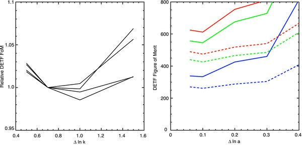
Figure 2 shows Δln k ≈ 0.7–1 yields minimum information for fixed RMS priors, but the dependence is very weak. The FoM varies by only 7% over the range 0.5 < Δln k < 1.5. We henceforth adopt Δln k = 1. Perhaps not surprisingly, this makes the nuisance functions have ≈1 independent node in each multipole bin of Δlog₁₀ℓ = 0.3.

Zoom In Zoom Out Reset image size

All of the nuisance functions are dependent on z. We next investigate the redshift node spacing Δln a at which the nuisance functions are most damaging to the DETF FoM. We find that the FoM is insensitive to the Δln a of the power-spectrum theory errors. The value of Δln a for the calibration functions f and q that minimizes the FoM depends upon the strength of the prior. The choice Δln a = 0.5 produces an FoM that is within 2% of the minimum, so we fix this value for the theory-error and calibration nuisance functions.

The redshift freedom given to the bias and intrinsic alignment nuisance functions has a strong impact on the DETF information content. Figure 2 illustrates that, at fixed RMS prior variation, models with freedom to vary on rather fine scales Δln a = 0.1 are most damaging to cosmological information.

Another approach is linear interpolation: choosing a spacing Δx = 2/(N − 1), we define a_i as the value of f at x_i = iΔx − 1. At some other x_i < x < x_i+1, we define

$$\begin{equation} f(x) = wa_i + (1-w) a_{i+1}, \qquad w={x_{i+1} - x \over \Delta x}. \end{equation} \tag{ A1 }$$

If we assign an independent Gaussian prior of width σ_a to each a_i, then by definition we have Var[f(x)] = σ²_a if x coincides with a node. But, the variance of f is not quite homogeneous: it drops to Var[f(x)] = σ²_a/2 when x is halfway between two nodes. If we want the mean variance of f(x) over the interval x ∈ [ − 1, 1] to equal σ²_f, then the variance of the prior on each node needs to be σ²_a = 3σ²_f/2.

Polynomial expansions are also commonly used to model nuisance functions. The simplistic form f(x) = ∑a_ixⁱ results in extremely nonuniform variance for f with diagonal prior on {a_i}, and hence is inappropriate for our purpose. A better choice is to expand in Legendre polynomials P_n(x), which are orthogonal over [ − 1, 1]. We define

$$\begin{equation} f(x) = \sum _{i=0}^{N-1} a_i P_i(\nu x). \end{equation} \tag{ A2 }$$

Recall that the Legendre polynomials satisfy P₀ = 1, P₁ = x, (n + 1)P_n+1 = (2n + 1)xP_n − nP_n−1.

We wish to choose priors {σ_i} on {a_i} that cause the variance of f(x) be as uniform as possible for x ∈ [ − 1, 1]. We have not found a way to attain perfect uniformity in x with polynomial interpolation; however, the following scheme gets usefully close. We discover numerically that

$$\begin{equation} \lim _{N\rightarrow \infty } {1 \over N} \sum _{i=0}^{N-1} P_n^2(\nu x) (2i+1) = {2 \over \pi } \left(1-\nu ^2x^2\right)^{-1/2}. \end{equation} \tag{ A3 }$$

This implies that if we set $\sigma _i = \sqrt{(2i+1)\pi /2N}$, then in the limit of large N we will obtain Var[f(x)] = (1 − ν²x²)^−1/2. For ν = 1, this would diverge at the ends of our nuisance function's interval. If, however, we choose ν = 0.9, the RMS is only ≈1.5 times larger at the endpoints than at x = 0. Over the [ − 1, 1] interval, the mean variance is (sin⁻¹ν)/ν. Hence, if we wish to have a function with 〈Varf(x)〉_x = σ²_f, we set the priors on the Legendre coefficients to be

$$\begin{equation} \sigma _i = \sigma _f \sqrt{(2i+1)\pi \nu \over 2N \sin ^{-1}\nu }. \end{equation} \tag{ A4 }$$

The Fourier, linear interpolation, and Legendre polynomial functional forms can each be extended to >1 dimensions in a straightforward fashion. In the lens modeling, we need functions of the following dimensions:

• 1.  
  comoving wavenumber or physical scale: x₁ = ln k;
• 2.  
  redshift z: more precisely, we will use the variable x₂ = ln(1 + z); and
• 3.  
  photometric redshift error Δz: more precisely, our code uses the variable x₃ = Δln(1 + z) = ln [(1 + z_α)/(1 + z_i)] for subset αi.

A.3.1. The kz Form

A.3.2. The zΔz Form

For nuisance variables over the (x₂, x₃) space (z and Δz), we adopt the following strategy: we choose to have variation over x₃ be described by polynomials since we usually define the range of noncatastrophic photo-z errors to be bounded to some range |x₃| ⩽ Δ_max. We define the "zΔz" functional form as follows:

$$\begin{equation} f(x_2,x_3) = \sum _{i=0}^{N-1} a_i(x_2) P_i(\nu x_3 / \Delta _{\rm max}). \end{equation} \tag{ A5 }$$

The Legendre coefficients are in turn defined to be linearly interpolated between a series of values a_ij at redshift nodes {ln(1 + z_j)}. The a_ij become parameters of the model.

The fiducial and prior values for the i = 0 terms (constant in x₃) are treated differently than the i > 0 terms. We might, for example, expect some nuisance functions to vary strongly with x₂ (nominal redshift) but only slightly with x₃ (photo-z error) at fixed x₂.

We specify the total RMS fluctuation in f allowed by the prior to be σ_f. But, we also specify the fraction VarFracDZ of the variance that is due to dependence on x₃. If we define

$$\begin{equation} \bar{f}(x_2) \equiv \int _{-\Delta _{\rm max}}^{+\Delta _{\rm max}} dx_3\,f(x_2,x_3) / 2\Delta _{\rm max}, \end{equation} \tag{ A6 }$$

then we aim to achieve

$$\begin{eqnarray} {\rm Var} [\bar{f}(x_2)] & = & \sigma ^2_f \left(1-{\tt VarFracDZ}\right), \end{eqnarray} \tag{ A7 }$$

$$\begin{eqnarray} {\rm Var} \left[f(x_2,x_3)-\bar{f}(x_2)\right] & = & \sigma ^2_f \left({\tt VarFracDZ}\right). \end{eqnarray} \tag{ A8 }$$

This is achieved approximately by setting the priors on the constant terms as

$$\begin{equation} \sigma ^2_{0j} = \frac{3}{2} \sigma ^2_f \left(1-{\tt VarFracDZ}\right) \end{equation} \tag{ A9 }$$

and the x₃ dependent terms (i > 0) as

$$\begin{equation} \sigma ^2_{ij} = \frac{3}{2} \sigma ^2_f \left({\tt VarFracDZ}\right) \sqrt{(2i+1)\pi \nu \over 2N \sin ^{-1}\nu }. \end{equation} \tag{ A10 }$$

The RMS prior variation σ_f can be made a function of x₂ without loss of generality. We typically take fiducial values of a_ij = 0 for i > 0 in our nuisance functions, i.e., no fiducial dependence upon Δz.

To summarize, the zΔz nuisance function is specified by

• 1.  
  the order N of the polynomial in x₃;
• 2.  
  the maximum range Δ_max of applicability in the x₃ axis;
• 3.  
  the spacing Δx₂ = Δln(1 + z) of the nodes for linearly interpolation in x₂;
• 4.  
  the RMS variation σ_f of the function allowed under the prior, which can depend on x₂;
• 5.  
  the fraction VarFracDZ of this variance that is due to x₃ (Δz) dependence; and
• 6.  
  the fiducial dependence of f on x₂.

A.3.3. The kzΔz Form

The bias and correlation coefficients can, most generally, depend on scale (x₁) as well as subset (x₂, x₃), so we generalize to the "kzΔz" functional form

$$\begin{equation} f(x_1,x_2,x_3) = \sum a_i(x_1,x_2) P_i(x_3). \end{equation} \tag{ A11 }$$

The coefficients a_i are linearly interpolated between nodes in the two-dimensional space (x₁, x₂). Thus, the free parameters of this model become the Legendre coefficients a_ijk. As for the zΔz function, we specify the prior by the overall mean RMS variation σ_f (which can be a function of x₂ and x₃), plus the VarFracDZ specifying how much of the variance is manifested as dependence on Δz. The formulae for the priors σ_ijk on the nodal coefficients are derived exactly as in Equations (A9) and (A10), except that we now need factors of (3/2)² to account for the reduced variance when interpolating in two dimensions.

The kzΔz function thus requires all of the specifications as the zΔz function plus a spacing Δln k for nodes in the x₁ axis.