


ABSTRACT
We demonstrate that the Oosterhoff II (Oo II) RR Lyrae ab variables are hotter by ∼270 K, at the same period, than Oo I variables. Or, at the same (〈B〉 − 〈V〉)0 value the Oo II variables have larger radii than Oo I variables. This accounts for the reason Oo II variables are brighter (0.12–0.20 mag) than Oo I variables. The dependence of the light amplitude of RR Lyrae variables on temperature is independent of Oo type. This makes it possible to derive an accurate set of equations to relate intrinsic (B − V)0 color indices to light amplitudes, which in turn can be used to determine the interstellar reddening (E (B − V)). With just a few variables (∼5), it is possible to determine the E (B − V) to an accuracy of <0.01 mag in the absence of systematic photometric errors. We discuss the errors introduced in color excess determinations by including the Blazhko stars in a solution. A comparison of color excess values of 23 globular clusters and two regions of the Large Magellanic Cloud (LMC), determined with the aid of our newly developed equations, are found to compare favorably (∼0.01 mag) with color excess values found in the literature. Four new Oo III variables, some found in metal-poor clusters, are discussed. An analysis of the galactic-field variables indicates the majority are Oo I and Oo II variables, but a few short-period (log P < −0.36) metal-strong variables, so far not found in galactic globular clusters are evidently ∼0.30 mag fainter than Oo I variables. Oo III variables may also be present in the field. We conclude that the RR Lyrae ab variables are primarily restricted to four sequences or groups. If we assume that the Oo I variables' mean absolute magnitude is Mv = 0.61, the mean absolute magnitudes of the other three sequences are: short-period variables Mv ∼ 0.89 mag, Oo II Mv ∼ 0.43 mag, and Oo III Mv ∼ 0.29 mag. The Oo I fundamental RR Lyrae ab red edge (FRE) and fundamental blue edge (FBE) occur at approximately the following temperatures: FRE T ∼ 6180 K and FBE T ∼ 6750 K. There is a strong dependence of Mv on [Fe/H] as we proceed from the short-period variables to the Oo I variables and to the Oo II variables, but there seems to be little or no dependence of Mv on [Fe/H] for stars within a group, at least for the Oo I and Oo II groups. The Oo II variables exhibit a weak period luminosity relation in V in many globular clusters unlike the Oo II-like variables in Oo I clusters which do not exhibit a P–L relation. The properties of some intermediate LMC clusters are discussed.
Export citation and abstract BibTeX RIS
1. INTRODUCTION
The RR Lyrae variable stars, found on the horizontal branch (HB) of globular clusters as well as in the field of galaxies, continue to play an important role in astronomy, as standard candles, for finding distances. They are old (∼12–13 Gyr), low-mass stars (∼0.5–0.7 solar masses) that derive their energy from core-helium burning. Apparently, they are radial-pulsating variables with periods ranging from 0.2 days to 1 day. Some evidence for nonradial pulsations has been made by several investigators. See the review by Moskalik (2013).
The variables were divided into classes a, b, and c based on their periods and light curve shape by Bailey (1902). The ab variables, now considered one group, have asymmetric light curves of long period and large amplitude compared to the more symmetrical shorter-period small amplitude c variables. It is now recognized that the ab variables are pulsating in the fundamental radial mode, while the c variables are pulsating in the shorter-period first-overtone radial mode.
Oosterhoff (1939, 1944) pointed out that some globular clusters have RR ab Lyrae stars with mean periods of ∼0.55 days and others with mean periods clustering around ∼0.65 days. The first group is now known as Oosterhoff type I clusters (Oo I), whereas the second group are known as Oosterhoff type II clusters (Oo II). When metal abundance determinations became available, it was recognized that while the variables all tend to be metal poor, the stars in Oo I clusters are more metal rich than the stars in Oo II clusters. Clusters that have stars with [Fe/H] values > −1.5 tend to be Oo I while clusters with stars that have [Fe/H] values < −1.5 are usually Oo II. The most metal-rich clusters frequently have only stars on the red side of the RR Lyrae stars and have few if any RR Lyrae variables. Sandage (1958) suggested that the Oo II HBs are more luminous than the HB of Oo I clusters. Bono et al. (2007), find that Oo II variables are brighter by ∼0.2 mag. A follow up on this suggestion by McNamara (2011) fully confirms the ∼0.20 mag difference and we will demonstrate in this paper that it is caused primarily by an increase of the temperature of Oo II variables of ∼270 K over the Oo I variables at the same period.
A large number of both theoretical and observational investigations have been devoted to better understanding issues related to the RR Lyrae stars. They include among others contributions by Bono & Stellingwerf (1994) and Bono et al. (1995), describing convective pulsating models. Other contributions, frequently using the convective model results in their discussions, include Caputo et al. (2000), Bono et al. (2002, 2003, 2007), Marconi et al. (2003, 2005), Di Criscienzo et al. (2004), and Cacciari et al. (2005). We will rely heavily on the results presented in these contributions in our discussion to follow.
More details beyond those described in our short introduction regarding RR Lyrae stars may be found in the introduction of the Marconi et al. (2003) contribution.
In this paper, we will discuss the cluster M3 in Section 2 pointing out that the evolved RR Lyrae stars are similar to RR Lyrae variables in Oo II clusters and set up equations to derive reddening of RR Lyrae stars from their light amplitudes. Section 3 is devoted to deriving reddening of a select group of globular clusters and making comparisons with other reddening values. Section 4 is devoted to discussing Oo I and Oo II stars in globular clusters. Section 5 is concerned with the Oo III stars. The galactic field variables are discussed in Section 6 and Section 7 is a discussion of the absolute magnitudes of the RR Lyrae stars. Section 8 is devoted to comments on Oo I and Oo II variables. Section 9 discusses the properties of some intermediate clusters of the Large Magellanic Cloud (LMC) and Section 10 is a summary of our conclusions.
2. THE GLOBULAR CUSTER M3
M3 (NGC 5272) is a galactic-halo cluster containing a large number of RR Lyrae stars. The new Harris catalog (Harris 1996, 2010 edition) lists the metallicity as [Fe/H] = −1.5 on the Carretta et al. (2009) scale placing it near the division of Oo I and Oo II clusters. It has long been considered the prototype Oo I cluster. However, with the discovery of evolved RR Lyrae stars brighter (∼0.12 mag) than most of the other variables (Clement & Shelton 1999a; Cacciari et al. 2005), it appears to have a few stars with Oo II characteristics. The most extensive discussion of the properties of this cluster is found in the Cacciari et al. paper in which one can find almost every point of interest discussed very carefully. The photometry discussed in the paper is very accurate, making it possible to draw firm conclusions. We are primarily interested in two issues: (1) comparing the temperatures of the Oo II-like variables with the temperatures of the majority of the variables that have Oo I characteristics and (2) attempting to utilize the light amplitude–(B − V)0 relations of the variables in M3 to determine the reddening of other clusters.
We begin with a discussion of the Bailey diagram (plot of light amplitude versus log P (P in days) of M3 shown in Figure 1. The periods of the RRab variables and their light amplitudes in the V band are found in Table 2 of Cacciari et al. (2005). The table excludes the Blazhko variables which are listed in their Table 3. This diagram has been discussed many times before, but is pertinent to our discussion here as well as in other sections of this investigation. The Oo I RRab variables are plotted as solid diamonds and nine of the stars that lie systematically above most of the variables (∼0.12 mag), referred to by Cacciari et al. (2005) as evolved stars, are shown as open squares. AV is the light amplitude in the V band where the minimum magnitude is measured from phase 0.5 to 0.8. At a given light amplitude, the nine stars are shifted systematically to longer periods, (∼0.063 in log P), and occupy a region of the diagram usually populated by Oo II cluster stars. Both sets of data points have been fit with second order polynomials. If the polynomials are extrapolated (by eye) to AV = 0.0, the corresponding log P values are ∼−0.16 (P = 0.69 days) and ∼−0.105 (P = 0.79 days). The B − V values at these log P values must correspond close to the color indices of the fundamental red edge (FRE) where the stars cease pulsating.
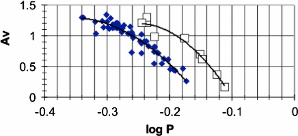
Figure 1. Period–amplitude diagram for normal RRab variables in the globular cluster, M3. Small solid diamonds are the Oo I stars, and the open squares are the Oo II-like stars (evolved variables according to CCC). Some of the data points lying below the curves may be unrecognized Blazhko variables. AV is the amplitude in the V photometric band.
Download figure:
Standard image High-resolution imageFigure 2 is a plot of the intrinsic, intensity-mean color indices (〈B〉 − 〈V〉)0 versus the log P values of the RRab variables (Table 2 of Cacciari et al. 2005), where we have calculated 〈B〉 − 〈V〉 from the 〈B〉 and 〈V〉 values listed for each star in the table and subtracted 0.01 mag to allow for the color excess of the cluster. We use the same symbols to designate the variables, solid diamonds for the Oo I star and the open squares for evolved variables. It is apparent that the evolved stars have smaller (〈B〉 − 〈V〉) values, that is, higher temperatures than the Oo I variables at the same period. This is also apparent in the third panel of Figure 5 of the Cacciari et al. contribution. The higher temperatures must be the reason that they are more luminous. The linear equations that fit the data points given in the figure corresponding to the lines are:
Equation (1) refers to the solid diamonds (Oo I stars) and Equation (2) to the open squares (evolved variables or Oo-like II stars). The amplitude versus (〈B〉 − 〈V〉)0 data discussed later suggests that the color index of the FRE is (〈B〉 − 〈V〉)0 ∼ 0.395 mag. This corresponds to log P = −0.175 (P = 0.668 days) for the Oo I stars and log P = −0.10 (P = 0.794 days) for the evolved variables. The FRE log P values agree closely with the value of log P = −0.16 and −0.105 values inferred from the V amplitude–log P diagram above.

Figure 2. (〈B〉 − 〈V〉)0–log P diagram of the RRab variables in the globular cluster M3. Small solid diamonds are Oo I variables and the open squares are the Oo II-like variables. Note at the same period, the B − V color indices of the Oo II-like variables are smaller, indicating higher temperatures and at the same radius, must be more luminous stars than the Oo I variables. Or at the same amplitude (temperature) the Oo II-like variables have longer periods and larger radii, and consequently, are brighter than the Oo I stars. The Oo II-like stars are typically brighter by 0.12–0.20 mag than Oo I variables.
Download figure:
Standard image High-resolution imageCacciari et al. (2005, CCC) discuss five different temperature scales (see their Table 4). We decided to utilize the Castelli (1998) scale in our discussion since it is sort of a mean of all five scales and is used in theoretical papers to be discussed later. A least-square fit to the Castelli data in CCC's Table 4 yields
The other temperature scales indicate that the errors in the temperatures given by this scale could easily be ±100 K. At log P = −0.2 ((B − V)0 = 0.368 mag Oo I, (B − V)0 = 0.309 mag Oo II), the differences in the color index indicate that the effective temperature of the evolved variables are 270 K greater than the Oo I variables. This increase in temperature makes them 0.18 mag more luminous than the Oo I variables if there is no change in radius. This is indeed the case since at a given abundance Z, the radius depends only on the period, P (see the PRZ relation in next paragraph). We can also find the difference in magnitude between the Oo I and Oo II-like variables by the difference in the log P values at the same given amplitude, AV. We will show later that the (B − V) values or temperatures of Oo I stars and Oo II-like stars are identical at the same amplitude regardless of period (P) as suggested indirectly by Bono et al. (1995) on theoretical grounds.
Starting with L/L☉ = R2 (Teff/Teff☉)4, we find that M(bol) = −5 log R − 10 log Teff + 42.37. The radius, R, is expressed in solar units and we adopted 5780 K and M(bol)☉ = 4.75 mag for the effective temperature and absolute-bolometric magnitude of the Sun. Marconi et al. (2005) find a period–radius–metallicity relation given by log R = 0.774 + 0.580 log P − 0.035 log Z. At Z = 0.001 ([Fe/H] ∼ −1.5), this equation becomes log R = 0.879 + 0.580 log P. It follows that M(bol) = −2.90 log P − 10 log T + 37.98. The magnitude difference between the Oo I and Oo II variables at the same temperature is given by ΔM(bol) = Δ (Mv) = Δ(–2.90 log P). At the amplitude of 0.6 mag, the log P values differ by 0.063 making the Oo II variables brighter by 0.18 mag in agreement with the value based on a temperature difference at constant R.
In as early as 1958, Sandage (1958) suggested that the RR Lyrae stars in Oo II clusters are brighter by 0.2 mag than the RR Lyrae stars in Oo I clusters. Clement & Shelton (1999a, 1999b) discuss in considerable detail the magnitude difference and period-shift effect between the two types of clusters. The whole issue of the period-shift effect and the nature of the Oosterhoff groups are summarized in Smith (1995 pp. 53–60). Two more recent discussions are found in Bono et al. (2007) and McNamara (2011).
We have designated different numbers of evolved variables in Figures 1 and 2 simply for the reason different numbers stand out in each diagram, indicating they are unusual, setting them apart from the Oo I variables. When the variables have large amplitudes it is often difficult to assign sequences and errors can easily be introduced. It is apparent that Figure 2 may be as good if not better, than Figure 1 in distinguishing the evolved stars from the Oo I variables. This is possible because the photometry is so accurate. The two stars (open squares) with log P values of ∼−0.3 in Figure 2 are not obvious in Figure 1 as evolved stars, but certainly fall on the line passing through the other stars designated by the open squares and are also among the luminous stars in the color–magnitude diagram (Figure 3, CCC).
The average period of the nine stars designated as evolved by CCC is 〈P〉 = 0.656 days (log 〈P〉 = −0.183). If they were the only RRab Lyrae stars in the cluster it would be classified as Oo II instead of Oo I. It appears that M3 is a transition cluster rater than a pure Oo I cluster. As pointed out previously, M3 has an extensive horizontal-blue branch, and as others have suggested it is tempting to suggest the evolved variables have evolved from this branch.
In Figure 3 we compare the intensity mean 〈B〉 − 〈V〉 color indices of the RR Lyrae ab variables with their AV amplitudes. As pointed by Bono & Stellingwerf (1994) and Bono et al. (1995) the height of the convective layer controls the amplitude of pulsation and since the height of the convection layer depends on the star's temperature the light amplitude correlates with temperature or on a color index such as 〈B〉 − 〈V〉. Again we make a distinction between the evolved or Oo II-like variables (open squares) and the Oo I variables (solid diamonds). All the data points, regardless of the Oo type of the variables, fall along the quadratic curve. This implies that if we try to utilize this curve to estimate the reddening of other globular clusters we can ignore the issue of whether the cluster is Oo I or Oo II. In later sections of this investigation we will also assume that the light amplitude uniquely gives the temperature of the Oo III variables as well as the metal-strong short-period RR Lyrae stars not found in globular clusters. Note that the scatter in the data points appears to increase at AV values >1.0 mag. The equation of the fitting curve is:
Marconi et al. (2003) have already commented on the high accuracy involved in using an equation similar to Equation (4) to determine reddening of similar clusters. In the present context, barring systematic errors, the reddening could be determined of an identical cluster, with photometry similar in accuracy of M3, with an error of ∼±0.012 mag with one star and an accuracy of ∼±0.002 mag with 40 stars. The dashed line lying generally above the data points is a fit to the static colors (the colors the stars would have in the absence of pulsation) found in Table 2 of CCC. The colors differ from the intensity mean colors. Note that the fit to the static colors is linear and the departure from linearity in the intensity-mean colors is due to the intensity-mean colors failing to correspond to static colors.
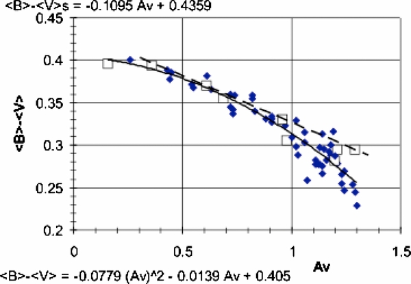
Figure 3. 〈B〉 − 〈V〉–AV amplitude diagram for normal RRab variables in M3. The symbols are the same as in Figures 1 and 2; small solid diamonds are Oo I variables and open squares are Oo II-like variables. The Oo I and Oo II-like variables fall on the same loci indicating one can ignore the issue of whether the star is Oo I or Oo II in using the amplitude to infer the intrinsic (〈B〉 − 〈V〉)0 color index or temperature of the star. The same also appears to be the case for Oo III variables as well as the short-period variables (log P < −0.35 days) not found in galactic globular clusters but found in the galactic field. This figure confirms the suggestions of Bono & Stellingwerf (1994) that the height of the convective zone, which in turn is a function of the temperature, controls the pulsation amplitude of the variable. The linear curve (dashed line) gives the 〈B〉 − 〈V〉 index if the stars did not exhibit pulsation (static color index).
Download figure:
Standard image High-resolution imageThe Castelli (1998) temperature scale and static colors (0.29 and 0.415) at the edges of the instability strip indicate the temperature of the FBE is 6750 K and the FRE is 6180 K, suggesting that the RR Lyrae ab instability strip is ∼570 K wide. The temperature of the FBE may actually be greater in an Oo I cluster than an Oo II cluster because the light amplitudes tend to be larger in Oo I clusters than in Oo II clusters near the FBE. Di Criscienzo et al. (2004) present in their Table 3, the period, color, and V amplitude of a fundamental model (Z = 0.001, M = 0.75, L = 1.61, M and L in terms of the Sun) as a function of two mixing lengths l/Hp = 1.5 and 2.0. The total width of the fundamental mode instability strip is dependent on the mixing length: 800 K for l/Hp = 1.5 and 700 K for l/Hp = 2.0. Although there is not an exact match of the models with the observational data, we can use period and amplitude differences to estimate the width of the instability strip of the RR Lyrae ab variables. We find ∼700 K and ∼650 K for the l/Hp = 1.5 models, and ∼700 K and ∼500 K for the l/Hp = 2.0 models, respectively. The average width (640 K) is slightly larger (∼70 K) than our initial estimate.
We present the following equations to calculate the intrinsic color indices of RRab Lyrae stars in globular clusters and galaxies. They are similar to equations already developed by Piersimoni et al. (2002). We will consider the metallicity correction later.
(〈B〉 − 〈V〉)0 and ((B − V)mag))0 are the intensity and magnitude mean-intrinsic B − V values of the variables, and AV, AB, and P are the amplitudes in the V and B bands and the period in days, respectively. Note that Equation (5) is identical to Equation (4) except for the constant term that differs by 0.01 mag. All of the equations were derived in a similar manner from the data given in Table 2 of CCC. In each equation, 0.01 mag was subtracted from the constant term to allow for the 0.01 mag reddening of the cluster. By comparing the observed color indices of RR Lyrae stars in the galactic field, and other clusters and galaxies, with those calculated from these equations the color excess, E (B − V), follows. We present these equations to cover all contingencies of the parameters that observers tabulate. The equations depend critically on the photometry of Cacciari et al. (2005) being free of systematic errors and on the color excess (0.01 mag) adopted by Cacciari et al. Piersimoni et al. (2002) estimate the color excess of M3 as E (B − V) = 0.011 mag, similar to the CCC value.
The referee has pointed out that the errors in the coefficients of the linear terms in Equations (5)–(8) are as large if not larger than the coefficients, suggesting that they are not necessary, only a second order term is required. Although true, we note that intensity mean-intrinsic B − V colors require a small negative linear term while the magnitude mean-intrinsic B − V colors require a small positive linear term to actually minimize the residuals.
We also have derived equations to determine the intrinsic color indices from the c variables. They exhibit a much smaller range in light amplitude and therefore, may not be quite as accurate as the equations of the RRab variables to determine reddening values. We removed three outlier stars (106, 178, and 203) from Table 1 of CCC and found that the following equations represent the intrinsic color indices very well.
Like the RRab equations ((5)–(9)), 0.01 mag has been subtracted from the constant terms to allow for reddening. The fit to the data points of Equation (11) is shown in Figure 4. Note again the evolved variables (open squares) fall with the other stars where as in an AB–log P, diagram they are well separated. Magnitude mean, ((B − V)mag)0, color indices of the c variables are systematically 0.009 ± 0.002 mag more positive than the intensity mean-color indices. The same set of equations, (10), (11), and (12), can therefore be used to calculate intrinsic magnitude-color indices by simply adding 0.009 mag to the values found from these equations. Normally, but not always, the AV amplitude and intensity mean magnitudes are tabulated by authors so Equations (5), (9), (10), and (11) should be the most useful.
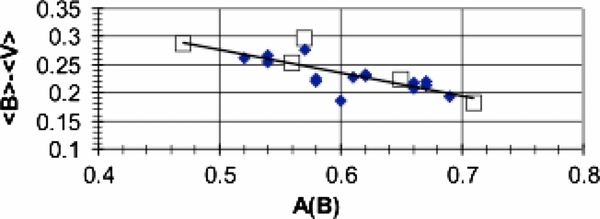
Figure 4. 〈B〉 − 〈V〉–A(B) (AB in the text) amplitude diagram for the RR Lyrae c variables in M3. Note that the Oo II-like variables (open squares) fall along the same line as the Oo I variables (small solid diamonds) similar to the RR Lyrae ab variables (Figure 3). A(B) is the amplitude in the B photometric band.
Download figure:
Standard image High-resolution imageWe now consider the corrections for metallicity. For the ab variables, the corrections are found from the galactic-field variables and from model atmospheres. Intrinsic B − V values of the field variables are plotted as a function [Fe/H] in Figure 11 of Sandage (2006). Although the data exhibits a large amount of scatter, a parabolic curve through the data points (not the curve given by Sandage) yielded the corrections given in Column 3 of Table 1 as a function of the [Fe/H] values given in Column 1. In addition, we calculated corrections from the Lejeune et al. (1998) tables which give color indices as a function of temperature, surface gravity (assumed to be log g = 2.75), and [Fe/H] values. These corrections are given in the second column. They are similar to the corrections given for the star data except for [Fe/H] values <−1.5. The model corrections (small negative values) behave according to expectation while the star data give positive corrections. We adopt the corrections given in the fourth column. Corrections for the c variables have also been calculated with the aid of the Lejeune et al. tables. They are about half that of the corrections for the ab variables, a consequence of their higher temperatures. No star data for calculating corrections for the c stars are available. We suggest using one-half the values given in the fourth column of Table 1, since the models give values differing by about two.
Table 1. Metallicity Corrections
| ab Var [Fe/H] | Model Corr. | Star Corr. | Adopted Corr. |
|---|---|---|---|
| 0 | 0.072 | 0.076 | 0.074 |
| −0.25 | 0.05 | 0.053 | 0.052 |
| −0.5 | 0.035 | 0.035 | 0.035 |
| −0.75 | 0.022 | 0.02 | 0.021 |
| −1 | 0.015 | 0.009 | 0.012 |
| −1.25 | 0.006 | 0.003 | 0.004 |
| −1.5 | 0 | 0 | 0 |
| −1.75 | −0.003 | 0.001 | 0 |
| −2 | −0.008 | 0.007 | 0 |
| −2.3 | −0.009 | 0.018 | 0 |
Download table as: ASCIITypeset image
In the process of calculating the color excess of NGC 3201, we discovered, as noted previously, that Piersimoni et al. (2002) had already derived empirical relations connecting the intrinsic B − V and V − I color indices to the AB light amplitude, pulsation period, and metallicity. They used the galactic field RR Lyrae ab stars to derive their equations. We will compare color excess values determined from our equations with the color excess values determined with the Piersimoni et al. equations and with other color excess determinations later.
2.1. The Blazhko Stars in M3
About one third of the RR Lyrae stars in M3 are classified as Blazhko variables by CCC. They are variables that exhibit modulations in their pulsation cycle over periods of several weeks to hundreds of days. Their light curves show variations in both amplitude and shape. Jurcsik et al. (2012) investigated the photometry of the RR Lyrae stars over a 120 yr time span and found that up to 50% of the light curves of RRab stars in M3 are not stable, some stars showing Blazhko modulations at only certain times. In many photometric studies of RR Lyrae stars, especially in clusters, the observational data are not extensive enough to identify all of the Blazhko stars so they will frequently be included in any bulk use of the variables. The question in our context is how the amplitude variations affect the reddening determinations from our basic set of equations that involve the light amplitudes.
We have used the Blazhko data in Table 3 (the same star because of amplitude changes can appear several times in the table) of CCC to derive an equation similar to our Equation (4). A plot of the Blazhko data in the 〈B〉 − 〈V〉–AV plane is shown in Figure 5. The heavy solid curve which is the best second-order equation to fit the data points is

The generally lighter upper dashed curve is the best fit (Equation (4)) to the normal RR Lyrae stars. For the most part, the Blazhko stars exhibit more scatter around the fitting curve and are shifted to smaller 〈B〉 − 〈V〉 values, compared to the normal RR Lyrae stars. Note, however, at the larger amplitudes, AV > 0.9 mag, the two curves give similar results (∼0.01 mag). We have calculated the color excess of the cluster employing only the Blazhko stars of Table 3 (CCC) (two outlier stars were removed) with the aid of Equation (5). We found E (B − V) = −0.010 mag. If the five stars with the largest σ's are removed the excess becomes −0.005 mag. Ideally of course, we should find a color excess of 0.01 mag. If we restrict our sample to just stars with AV > 0.9 mag, the color excess is E (B − V) = 0.009 ± 0.004 mag (n = 38 stars). Restricting the sample to stars with AV > 0.8 mag yields E (B − V) = 0.004 ± 0.004 mag (n = 48 stars). When the Blazhko stars have small amplitudes, they predict larger intrinsic (B − V)0 color indices and when compared with observed (B − V) values lead to smaller color excess values. We conclude that the inclusion of Blazhko stars in color excess determinations will increase the scatter in the data and may introduce a very small systematic error in E (B − V). Since they are usually a minority (∼1/3 or less) of the stars in a cluster in a typical data set, by excluding a few of the outlier stars in an analysis for color excess, one can correct for their small influence on a color excess determination. It is advisable to exclude them where possible, especially the small-amplitude variables, to attain the highest accuracy. To determine the most accurate E (B − V) from a Blazhko variable, it is advisable to use data when the star is near its maximum amplitude, when it is most similar to a normal RRab variable.
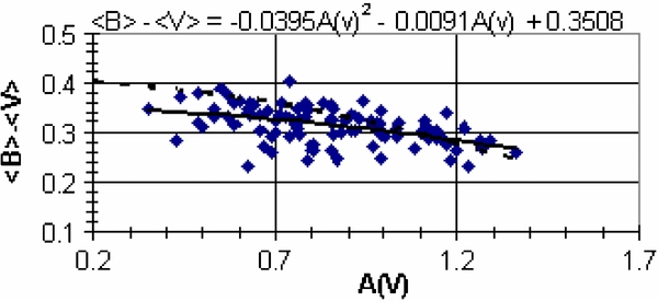
Figure 5. 〈B〉 − 〈V〉–A(V) diagram of the Blazhko variables in M3. The same Blazhko variable may appear as many as three times in the diagram due to its amplitude variation over time. The heavy solid curve is the best fit to the Blazhko variables (Equation (13) in the text) and the lighter (generally upper) dashed curve is the best fit to the normal RR Lyrae ab variables (Equation (4) in the text). Note that for large amplitudes (when the Blazhko stars are near their maximum amplitudes) the curves intersect.
Download figure:
Standard image High-resolution imageWe have plotted the AV amplitudes of the Blazhko stars against their log P values (Bailey diagram) in Figure 6. The result, as expected, is a scatter diagram. The two curves plotted are the Oo I (left) and Oo II (right) sequences of the normal RR Lyrae ab stars (Figure 1) for M3 which are not delineated by the Blazhko stars. Note that no Blazhko star data points fall above the Oo II curve and for the most part, have amplitudes smaller than the regular stars that define the two curves. This result is in agreement with Teays (1993) suggestion that when the Blazhko effect is present, it tends to reduce rather than extend the normal height of the maximum of the light curves of RR Lyrae stars.
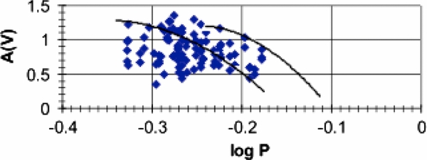
Figure 6. Period–amplitude diagram (A(V) = AV in the text) of the Blazhko variables in M3. The two curves in the diagram are the Oo I (left) and Oo II-like (right) loci delineated by the normal RR Lyrae variables (Figure 1). The Blazhko stars produce a scatter diagram with the majority of the data points falling below the Oo I curve and there are no data points above or to the right of Oo II-like curve, confirming earlier suggestions that the Blazhko effect tends to reduce the amplitude and does not increases the amplitude.
Download figure:
Standard image High-resolution imageOf particular interest is the large number of Oo I Blazhko stars, (M3), in the period range log P = −0.33 to −0.245 that show large departures from the Oo I curve for normal variables. At log P > −0.25, the Blazhko stars all fall very close to the normal curve or may be Oo II variables. Note that there are few if any Blazhko stars with periods larger than log P = −0.180.
3. REDDENING DETERMINATION OF OTHER CLUSTERS
We selected 18 galactic globular clusters, 5 LMC globular clusters, and 2 regions of the LMC with RR Lyrae stars to determine the reddening with the equations developed in the last section. We included known Blazhko stars in the analysis if they were included in tables published by authors and flagged, but not if they were published in separate tables. In many cases, the observing time frame was obviously not sufficient to identify all the Blazhko variables. In many cases, the amplitudes of the variables may have been determined by different methods than those employed by CCC. We made no attempt to correct the amplitudes. The objects are listed according to their NGC numbers or name in Column 1 of Table 2. The fields A and B of the LMC are the regions of the LMC observed by Clementini et al. (2003). Columns 2–9 list the color excess, E (B − V), calculated with the aid of the equations designated at the header of the column. The second header indicates the parameter or parameters used in the equation and whether intensity or magnitude means are used. The errors listed are the standard deviation of the mean values. Column 10 lists the average or "best" color excess and standard deviation based on the entries of the previous columns. In most cases, we gave greater weight to the excess values based on the ab variables. In many cases, the c variables give systematically different E (B − V) values up to ∼0.03 mag compared to the ab values. The c variables in these cases did not occupy the same region of the AV–log P diagram as the variables in M3, and we anticipate spurious results. Note that all five equations (Equations (5)–(9)) give very similar values for the ab variables. Columns 11 and 12 list the number of ab and c variables used in the analysis and reference to the contributions describing the observed properties of the variables, respectively. The data analyzed are a "mixed bag" and systematic errors in the various photometry of ∼0.01–0.03 mag may be present. The errors in the mean excess values are more realistically of ∼±0.008 mag rather than the typical ±0.002 to ±0.004 mag listed. An example is NGC 1466 where the (B − V) values of Walker (1992b) are systematically ∼0.03 mag smaller than the (B − V) values of Kuehn et al. (2011). An analysis of the Walker data gave E (B − V) = 0.059 mag compared to E (B − V) = 0.088 mag found from the Kuehn et al. photometry and reported in Table 2. Thus, a more appropriate excess value for NGC 1466 may be the average E (B − V) = 0.075 mag, rather than the value given in Tables 2 and 3.
Table 2. Color Excesses of Globular Star Clusters
| Cluster | ab Equation (5) A(V) | ab Equation (6) A(B) | ab Equation (7) A(V) | ab Equation (8) A(B) | ab Equation (9) A(V) | c Equation (10) A(V) | c Equation (11) A(B) | c Equation (12) A(V) | 〈E(B − V)〉 | N(ab)N(c) | References |
|---|---|---|---|---|---|---|---|---|---|---|---|
| int. E (B − V) | int. E (B − V) | mag E (B − V) | mag E (B − V) | Per. E (B − V) | int. E (B − V) | int. E (B − V) | Per. E (B − V) | ||||
| (mag) | (mag) | (mag) | (mag) | (mag) | (mag) | (mag) | (mag) | (mag) | |||
| 1466 LMC | 0.091 ± 0.008 | 0.090 ± 0.008 | 0.082 ± 0.008 | 0.093 ± 0.008 | 0.093 ± 0.008 | 0.092 ± 0.015 | 0.086 ± 0.017 | 0.092 ± 0.014 | 0.088 ± 0.002 | 25 10 | Kuehn et al. (2011) |
| Reticulum | 0.020 ± 0.004 | 0.020 ± 0.005 | 0.028 ± 0.004 | 0.056 ± 0.023 | 0.052 ± 0.019 | 0.028 ± 0.004 | 19 9 | Walker (1992a) | |||
| 1835 LMC | 0.065 ± 0.015 | 0.077 ± 0.017 | 0.065 ± 0.014 | 0.076 ± 0.013 | 0.081 ± 0.012 | 0.072 ± 0.004 | 13 13 | Walker (1993) | |||
| 1841 LMC | 0.152 ± 0.005 | 0.140 ± 0.009 | 0.140 ± 0.009 | 0.192 ± 0.008 | 0.188 ± 0.007 | 0.162 ± 0.012 | 12 4 | Walker (1990) | |||
| 2257 LMC | 0.031 ± 0.006 | 0.031 ± 0.007 | 0.029 ± 0.007 | 0.029 ± 0.008 | 0.018 ± 0.006 | 0.041 ± 0.007 | 0.043 ± 0.006 | 0.037 ± 0.006 | 0.032 ± 0.003 | 24 18 | Nemec et al. (2009) |
| LMC (A) | 0.106 ± 0.005 | 0.106 ± 0.005 | 0.100 ± 0.005 | 0.102 ± 0.006 | 0.107 ± 0.005 | 0.096 ± 0.010 | 0.093 ± 0.011 | 0.102 ± 0.008 | 0.102 ± 0.002 | 45 21 | Clementini et al. (2003) |
| LMC (B) | 0.075 ± 0.006 | 0.075 ± 0.006 | 0.075 ± 0.005 | 0.075 ± 0.005 | 0.087 ± 0.007 | 0.079 ± 0.009 | 0.078 ± 0.008 | 0.084 ± 0.007 | 0.078 ± 0.002 | 28 19 | Clementini et al. (2003) |
| NGC 104 | 0.068 | 0.066 | 0.066 | 0.064 | 0.019 | 0.063 ± .005 | 1 0 | Carney et al. (1993) | |||
| 1851 | 0.024 ± 0.006 | 0.036 ± 0.006 | 0.033 ± 0.005 | 0.033 ± 0.004 | 0.042 ± 0.006 | 0.042 ± 0.010 | 0.036 ± 0.008 | 0.045 ± 0.008 | 0.036 ± 0.002 | 19 7 | Walker (1998) |
| 3201 | 0.300 ± 0.006 | 0.303 ± 0.006 | 0.302 ± 0.006 | 0.304 ± 0.006 | 0.307 ± 0.005 | 0.316 ± 0.009 | 0.321 ± 0.002 | 0.304 ± 0.002 | 0.304 ± 0.002 | 50 2 | Piersimoni et al. (2002) |
| 4590 | 0.062 ± 0.055 | 0.064 ± 0.055 | 0.058 ± 0.055 | 0.059 ± 0.055 | 0.035 ± 0.055 | 0.079 ± 0.005 | 0.091 ± 0.006 | 0.073 ± 0.004 | 0.075 ± 0.008 | 2 26 | Walker (1994) |
| 5053 | 0.030 ± 0.022 | 0.020 ± 0.021 | 0.018 ± 0.017 | 0.056 ± 0.001 | 0.036 ± 0.013 | 0.046 ± 0.003 | 0.024 ± 0.004 | 6 3 | Nemec et al. (1995) | ||
| 5286 | 0.231 ± 0.019 | 0.228 ± 0.020 | 0.246 ± 0.023 | 0.237 ± 0.013 | 0.222 ± 0.006 | 0.233 ± 0.004 | 20 21 | Zorotovic et al. (2010) | |||
| 5466 | 0.003 ± 0.007 | −0.003 ± 0.007 | 0.000 ± 0.008 | −0.005 ± 0.007 | −0.018 ± 0.004 | 0.005 ± 0.031 | −0.007 ± 0.020 | −0.012 ± 021 | −0.005 ± 0.002 | 13 6 | Corwin et al. (1999) |
| 5904 | 0.039 ± 016 | 0.039 ± 0.016 | 0.041 ± 0.014 | 0.041 ± 0.014 | 0.034 ± 0.017 | 0.027 ± 0.008 | 0.034 ± 0.007 | 0.036 ± 0.008 | 0.036 ± 0.002 | 6 4 | Storm et al. (1991) |
| 6266 | 0.521 ± 0.008 | 0.522 ± 0.008 | 0.518 ± 0.008 | 0.519 ± 0.008 | 0.538 ± 0.008 | 0.506 ± 0.014 | 0.501 ± 0.015 | 0.522 ± 0.013 | 0.518 ± 0.004 | 67 32 | Contreras et al. (2010) |
| 6341 | 0.032 ± 0.004 | 0.020 ± 0.009 | 0.027 ± 0.010 | 0.019 ± 0.010 | 0.018 ± 0.011 | 0.023 ± 0.002 | 6 0 | Carney et al. (1992) | |||
| 6441 | 0.496 ± 0.007 | 0.502 ± 0.007 | 0.452 ± 0.008 | 0.416 ± 0.014 | 0.431 ± 0.013 | 0.416 ± 0.013 | 0.502ab | 26 12 | Pritzl et al. (2001) | ||
| 6388 | 0.396 ± 0.027 | 0.403 ± 0.026 | 0.4 | 4 0 | Pritzl et al. (2002) | ||||||
| 6715 | 0.172 ± 0.006 | 0.171 ± 0.006 | 0.161 ± 0.006 | 0.160 ± 0.006 | 0.178 ± 0.007 | 0.165 ± 0.019 | 0.156 ± 0.020 | 0.168 ± 0.020 | 0.167 ± 0.002 | 47 11 | Sollima et al. (2010) |
| 6809 | 0.121 ± 0.019 | 0.109 ± 0.105 | 0.106 ± 0.020 | 0.106 ± 0.016 | 0.111 ± 0.004 | 4 7 | Olech et al. (1999) | ||||
| 6864 | 0.164 ± 0.030 | 0.157 ± 0.037 | 0.161 ± 0.035 | 0.156 ± 0.041 | 0.159 ± 0.034 | 0.150 ± 0.027 | 0.145 ± 0.035 | 0.163 ± 0.024 | 0.158 ± 0.002 | 7 4 | Corwin et al. (2003) |
| 7078 | 0.117 ± 0.007 | 0.112 ± 0.007 | 0.107 ± 0.009 | 0.107 ± 0.009 | 0.107 ± 0.008 | 0.110 ± 0.002 | 26 0 | Corwin et al. (2008) | |||
| NGC 7089 | 0.024 ± 0.006 | 0.022 ± 0.007 | 0.016 ± 0.006 | 0.015 ± 0.007 | 0.003 ± 0.005 | 0.036 ± 0.019 | 0.033 ± 0.015 | 0.036 ± 0.014 | 0.023 ± 0.004 | 18 9 | Lee & Carney (1999) |
| Rup 106 | 0.134 ± 0.016 | 0.147 ± 0.012 | 0.146 ± 0.008 | 0.144 ± 0.006 | 0.141 ± 0.016 | 0.142 ± 0.002 | 7 0 | Kaluzny et al. (1995) |
Download table as: ASCIITypeset image
Table 3. Comparison of Color Excess Values
| Cluster | Other | [Fe/H] | 〈E (B − V)〉 | corr. E (B − V) | Harris E (B − V) | FIR E (B − V) | PBR E (B − V) | Authors E (B − V) | Pres − Har Diff | Pres − FIR Diff | Pres − PBR Diff |
|---|---|---|---|---|---|---|---|---|---|---|---|
| (mag) | (mag) | (mag) | (mag) | (mag) | (mag) | (mag) | (mag) | (mag) | |||
| 1466 LMC | −1.85 | 0.088 ± 0.002 | 0.088 | . | 0.09 | ||||||
| Reticulum | GLC 0435 | −1.7 | 0.028 ± 0.004 | 0.028 | 0.03 | ||||||
| 1835 LMC | −1.8 | 0.072 ± 0.004 | 0.072 | 0.13 | |||||||
| 1841 LMC | −2.2 | 0.162 ± 0.012 | 0.162 | 0.18 | |||||||
| 2257 LMC | −1.8 | 0.032 ± 0.003 | 0.032 | ||||||||
| LMC (A) | ∼−1.5 | 0.102 ± 0.002 | 0.102 | 0.116 | |||||||
| LMC (B) | ∼−1.5 | 0.078 ± 0.002 | 0.078 | 0.086 | |||||||
| 104 | 47 Tuc | −0.72 | 0.063 ± 0.005 | 0.039 | 0.04 | 0.03 | −0.001 | 0.009 | |||
| 1851 | −1.18 | 0.036 ± 0.002 | 0.03 | 0.02 | 0.04 | 0.04 | 0.02 | 0.01 | −0.01 | −0.01 | |
| 3201 | −1.59 | 0.304 ± 0.002 | 0.304 | 0.24 | 0.26 | 0.3 | 0.3 | 0.064 | 0.044 | 0.004 | |
| 4590 | M68 | −2.23 | 0.075 ± 0.008 | 0.075 | 0.05 | 0.06 | 0.05 | 0.025 | 0.015 | 0.025 | |
| 5053 | −2.27 | 0.024 ± 0.004 | 0.024 | 0.01 | 0.02 | 0.014 | 0.004 | ||||
| 5286 | −1.69 | 0.233 ± 0.004 | 0.233 | 0.24 | 0.29 | −0.007 | −0.057 | ||||
| 5466 | −1.98 | −0.005 ± 0.002 | 0 | 0 | 0.02 | 0.01 | 0 | −0.02 | −0.01 | ||
| 5904 | M5 | −1.29 | 0.036 ± 0.002 | 0.033 | 0.03 | 0.1 | 0.04 | 0.003 | −0.067 | −0.007 | |
| 6266 | M62 | −1.18 | 0.518 ± 0.004 | 0.51 | 0.47 | 0.46 | 0.04 | 0.05 | |||
| 6341 | M92 | −2.31 | 0.023 ± 0.002 | 0.023 | 0.02 | 0.02 | 0.003 | 0.003 | |||
| 6388 | −0.55 | 0.4 | 0.368 | 0.37 | 0.41a | −0.002 | |||||
| 6441 | −0.46 | 0.502ab | 0.465 | 0.47 | 0.61a | 0.53 | −0.005 | −0.065 | |||
| 6715 | M54 | −1.49 | 0.167 ± 0.002 | 0.167 | 0.15 | 0.15 | 0.16 | 0.017 | 0.017 | ||
| 6809 | M55 | −1.94 | 0.111 ± 0.004 | 0.111 | 0.08 | 0.14 | 0.11 | 0.031 | −0.029 | ||
| 6864 | M75 | −1.29 | 0.158 ± 0.002 | 0.155 | 0.16 | 0.15 | −0.005 | 0.005 | |||
| 7078 | M15 | −2.37 | 0.110 ± 0.002 | 0.11 | 0.1 | 0.11 | 0.01 | 0 | |||
| 7089 | M2 | −1.65 | 0.023 ± 0.004 | 0.023 | 0.06 | 0.04 | 0.01 | −0.037 | −0.017 | 0.013 | |
| Rup 106 | −1.68 | 0.142 ± 0.002 | 0.142 | 0.2 | 0.17 | 0.15 | 0.2 | −0.058 | −0.028 | −0.008 |
Note. aLow galactic latitude clusters in which the Schlegel maps give large reddening values.
Download table as: ASCIITypeset image
In Table 3, we make a comparison of our reddening values with other values in the literature. The objects studied are listed in the same order as in Table 2. Other frequently more familiar designations of the clusters are given in Column 2. The metallicities, [Fe/H], are listed for each object in Column 3. Note that the [Fe/H] values of the galactic globular clusters are from the Harris 1996 (2010 edition) catalog (Carretta et al. 2009 scale) while the [Fe/H] values for the LMC clusters (frequently on the Zinn & West 1984 scale) are found in the original papers listed in the last column of Table 3. They are not on the same system but any differences are small (⩽0.2). In Column 4, we list our color excess values found in Column 10 of Table 2. These values, corrected for metallicity according to the corrections given in Table 1, are given in Column 5. Note that the sign (+ or −) of the corrections given in Table 1 is appropriate when calculating intrinsic color indices. If they are applied at the color excess stage, as we have done, they are applied with the opposite sign.
Color excess values in the literature are presented in columns 6–9 of Table 3. Column 6 lists the color excess values listed in the Harris (1996, 2010 edition) catalog that are mainly inferred from color–magnitude diagrams of the clusters. The E (B − V) values (FIR) given in Column 7 were obtained from the Schlegel et al. (1998) reddening maps by Dutra & Bica (2000). E (B − V) values listed under PBR are inferred by equations similar to ours by Piersimoni et al. (2002) PBR. Finally, a few E (B − V) inferred by authors are given in Column 9. Note that the color excess values determined by methods other than color–magnitude diagrams are very valuable because they help in eliminating any circular reasoning involved in interpreting properties of the clusters from color–magnitude diagrams that in turn may depend on the reddening. We find the following differences between E (B − V) data sets in the sense of the present – others: 0.006 ± 0.006, n = 18, Harris; −0.005 ± 0.008, n = 16, FIR; and −0.007 ± 0.009, n = 8, PBR; where the uncertainty is the standard deviation of the mean value and n is the number of clusters. NGC 6441 and NGC 6388 were excluded from the FIR comparisons, because of their low galactic latitude.
Nemec et al. (2011) give AV light amplitudes, two values of the intrinsic (B − V) color index, and metallicity estimates for 19 RR Lyrae stars observed with the Kepler Space Telescope (see their Tables 5 and 4). We eliminated four metal-strong variables because the [Fe/H] values show such a large scatter that it is impossible to accurately correct the (B − V) colors for metallicity. The 15 remaining stars all fall in the [Fe/H] regime where corrections are very small or negligible. We adopted Nemec et al. AV values and calculated intrinsic (B − V) values with our Equation (6). We find the following average (B − V)0 difference between the 15 variables, present – others: 004 ± 0.002 mag, maximum difference 0.022 mag, J98 column; 0.000 ± 0.002 mag, maximum difference 0.016 mag, KW01 column. The average differences are <0.01 mag in all five comparisons with an average difference of 0.000 ± 0.002 mag.
The good agreement in these comparisons indicate that the adoption of the CCC photometry, along with the a color excess of 0.01 mag for M3 to develop Equations (5)–(9) to determine color excess values, does not introduce any large systematic errors in the E (B − V) values derived from the equations. A larger source of errors are the systematic errors in the photometry of the variables in the clusters.
4. THE PRESENCE OF Oo II STARS IN Oo I CLUSTERS AND Oo I STARS IN Oo II CLUSTERS
Is M3 unique in having a mix of Oo I and Oo II-like stars? We found that three predominately Oo I clusters (M3, M62, and M54) with [Fe/H] in the range of −1.18 to −1.5, that have extended blue-HBs and a large number of RRab variables, all contain some Oo II-like stars. In Figure 7, we show the RR Lyrae ab variables of M62 in the (〈B〉 − 〈V〉)0–log P plane. The distribution of the variables is similar to the M3 variables (see Figure 2). The Oo II-like variables (open squares) fall systematical about 0.05 mag less in 〈B〉 − 〈V〉 than the corresponding values of the Oo I variables (small solid diamonds). We find the average periods of the variables are 〈P〉Oo I = 0.547 days (M62) and 0.571 days (M54); 〈P〉Oo II = 0.636 days (M62) and 0.707 days (M54). In both of these clusters, as in M3, the Oo II-like stars are systematically brighter than the Oo I stars: 〈V〉Oo I = 16.29 ± 0.03 mag, (n = 56 stars), 〈V〉Oo II = 16.08 ± 0.05 mag, (n = 9 stars), M62; 〈V〉Oo I = 18.10 ± 0.06 mag, (n = 43 stars), 〈V〉Oo II = 17.96 ± 0.08 mag, (n = 11 stars), M54. Note that all three clusters have large numbers of RR Lyrae variables. NGC 3201, which is also an Oo I cluster with a large number of variables, has three stars that could be Oo II-like variables, but the scatter in the data is so large that it is hard to be certain. The Oo I clusters, M5 and M75, have blue-HBs but few RRab variables (n = 6 and 7, respectively), consequently the chances of finding Oo II-like variables are small and none are evident. The ratio of the number of Oo I variables to Oo II-like variables in the three clusters is similar. The ratios are 6.0 (M3), 6.2(M62), and 3.9 (M54). Uncertainties in the ratios arises because of the difficulty in eliminating Blazhko variables.

Figure 7. (〈B〉 − 〈V〉)0−log P diagram of the RR Lyrae variables (ab) in the globular cluster M62. The cluster has both Oo I (small solid diamonds) and Oo II-like variables (open squares). The two solid curves are similar to the corresponding curves of M3 (see Figure 2). It evident, that as in M3, the Oo II-like stars should be brighter than the Oo I stars.
Download figure:
Standard image High-resolution imageMost of the Oo II clusters have a small number of RR Lyrae ab variables. A perusal of the clusters reveal that there is no hard evidence of Oo I stars present in any of them. The three clusters with the largest number of variables in our study are NGC 5286 ([Fe/H] = −1.69), M15 ([Fe/H] = −2.37), and M2 ([Fe/H] = −1.65). Both the Bailey diagram and the (B − V)0–log P plot indicate a possibility that three stars in NGC 5286 could be Oo I stars but the observational scatter is large enough to cast doubt on this possibility. Similar diagrams of M2 and M15 indicate that if Oo I variables are present, it could only be at the short periods (log P < −0.25) where it is hard to distinguish between the two types of variables. Our sample is small so our tentative conclusion may be shown to be incorrect when additional accurate photometry of variables in similar clusters becomes available. In fact, ω Cen, which is classified as Oo II, does have a significant population of both Oo II variables as well as Oo I variables (McNamara 2011). This differs from the apparent tendency of Oo II clusters to have only Oo II variables. This may be additional evidence to support the idea that ω Cen is really a dSph galaxy rather than a globular cluster.
5. THE OSTERHOFF III VARIABLES
The possibility of a new Oo group beyond those introduced by Oosterhoff was suggested by Pritzl et al. (2000, 2001, 2002). They found that the RR Lyrae stars in the metal-rich clusters, NGC 6441 and NGC 6388, exhibited unique characteristics setting them apart from RR Lyrae stars in ordinary Oo I and Oo II clusters. The RRab variables in the clusters are metal strong, but have unusually long periods, contrary to the normal tendencies of the metal-strong variables being restricted to the shorter-period variables. Furthermore, according to theoretical models, the Oo III RRab variables should be somewhat brighter than the RRab variables in Oo II clusters. This is contrary to the usual view that the metal-strong variables are the least luminous. Because of these anomalies, the two clusters are sometimes termed Oo III. We will adopt this description in our discussion.
We have identified four stars in other clusters that are unique and apparently have similar properties. They are listed in Table 4. The star number is given in the first column, and the cluster is identified in the second column. The period, amplitude in the V band, and the intensity mean magnitudes 〈V〉 of the Oo III variable are given in columns 3, 4, and 5, respectively. The average 〈V〉 magnitude of the other RRab stars in the cluster and magnitude difference between the magnitude of the other RR Lyrae ab variables of the cluster and the 〈V〉 magnitude of the Oo III variable are given in Columns 6 and 7, and shows that the Oo III stars are brighter. The intrinsic B − V color indices of the Oo III variable, assuming the star's [Fe/H] value is −1.5, are listed in Column 8. The cluster's [Fe/H] value and cluster type are listed in the last two columns. We note that Pritzl et al. (2001) have already pointed out that V9 in 47 Tuc falls in the same region of the period–amplitude diagram as the RRab variables in NGC 6441 and 6388.
Table 4. Oosterhoff III Stars
| Star | Cluster | log P | AV | 〈V〉star | 〈V〉clus | ΔV | (〈B〉 − 〈V〉)0 | [Fe/H]clus | Type Cluster |
|---|---|---|---|---|---|---|---|---|---|
| (mag) | (mag) | (mag) | (mag) | (mag) | |||||
| V10 | M2 | −0.0576 | 0.634 | 15.73 | 15.95 | 0.22 | 0.355 | −1.65 | Oo II |
| V 9 | 47 Tuc | −0.1362 | 1.07 | 13.672 | 14.1 | 0.43 | 0.291 | −0.72 | Oo I |
| NV12 | NGC 5286 | −0.0433 | 0.41 | 16.251 | 16.57 | 0.32 | 0.359 | −1.69 | Oo II |
| NV10 | M75 | −0.0758 | 0.6 | 17.432 | 17.7 | 0.27 | 0.359 | −1.2 | Oo I |
Download table as: ASCIITypeset image
We have plotted the data of these stars in Figures 8 and 9. In Figure 8 (Bailey diagram), the four stars fall well to right of both the Oo II-like variables (open squares) and the Oo I variables (solid diamonds), indicating that the separate classification, Oo III, is certainly appropriate. The displacement of the Oo III variables to the right (increasing period) in the AV–log P diagram by ∼0.07 mag in log P implies that they are ∼0.20 magnitude brighter than Oo II variables,consistent with the ΔV values in Table 4. If we extrapolate the curves to zero amplitude, it is evident that the period of the FRE is different for each Oo type. This figure along with others indicates that the log P values of the (FRE's) are ∼−0.175 (P = 0.668 days) Oo I, ∼−0.100 (P = 0.794 days) Oo II, and ∼−0.02 (P = 0.955 days) Oo III. Although we have not discussed the fundamental blue edges (FBE), it is likely that they occur at increasing log P values as we proceed from Oo I to Oo III as well. The corresponding (〈B〉 − 〈V〉)0 values at the (FRE), at [Fe/H] = −1.5, would all be ∼0.395 mag. At identical log P values, the amplitude of the Oo II variables is larger than Oo I variables and the Oo III variables are larger than the Oo II variables. Since the (〈B〉 − 〈V〉)0 color indices are inversely correlated with the amplitude, this implies smaller (〈B〉 − 〈V〉)0 values corresponding to higher temperatures and consequently, more luminous variables as we proceed from Oo I to Oo III. This is clearly evident in Figure 9 where we use the same symbols as in Figure 1 to designate the various Oo types. At log P = −0.20, the (〈B〉 − 〈V〉)0 of the Oo II-like variables are ∼0.06 mag smaller than the (〈B〉 − 〈V〉)0 values of the Oo I variables. At log P = −0.125, the Oo III variables (〈B〉 − 〈V〉)0 values are ∼0.06 mag smaller than the (〈B〉 − 〈V〉)0 mag values of the Oo II-like variables.
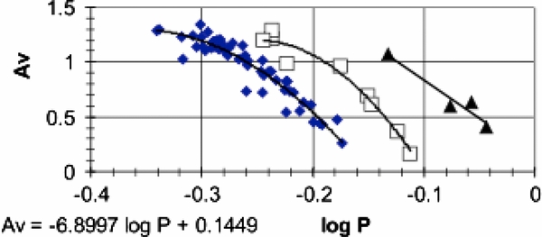
Figure 8. Position of four Oo III variables (solid triangles) in the AV–log P diagram (Bailey diagram). The two curves and data points on the left are for M3 (identical to Figure 1). The four stars are from globular clusters with different element abundances and Oo classes, and are the brightest RR Lyrae star in each of their clusters. Their position in the diagram indicates they are ∼0.20 mag brighter than the M3 Oo II variables. The equation is the fit to the four stars.
Download figure:
Standard image High-resolution image
Figure 9. Position of the Oo III variables (triangles) in the (〈B〉 − 〈V〉)0–log P diagram. Note the (〈B〉 − 〈V〉)0 values of the Oo III variables are smaller than the (〈B〉 − 〈V〉)0 values (open squares) of the Oo II-like variables at the same period, and thus must be more luminous if the radii are similar. The equation is the fit to the four Oo III stars.
Download figure:
Standard image High-resolution imageThe Oo III variables discussed by Pritzl et al. (2000, 2001, 2003) are all relatively metal-strong variables ([Fe/H] ∼ −0.5 to −0.7). If V10 in M2 ([Fe/H] = −1.65) and N12 in NGC 5286 ([Fe/H] = −1.69) are similar in metallicity to the other variables in these clusters, it would imply that Oo III stars can also occur for metal-weak stars.
6. THE GALACTIC-FIELD VARIABLES
We have selected 18 field stars listed in Table 4 of Piersimoni et al. (2002) and 65 variables studied by Lub, but listed by Sandage (1990) to investigate the classification of the field variables. Only AB amplitudes are tabulated in the Lub data set. We converted these values to AV amplitudes with the equation

The equation was derived with the aid of the AV and AB values of stable RR Lyrae ab variables in M3 (CCC). Bailey diagrams (AV amplitude versus log P) of each group are displayed in Figures 10 and 11. Of the 18 stars plotted in Figure 10, 12 stars are Oo I, 3 are Oo II, and 3 are metal-strong short-period stars (SW And [Fe/H] = −0.15, RR Gem [Fe/H] = −0.20, and AV Peg [Fe/H] = 0.00) and form another grouping displaced ∼0.105 in log P to smaller periods. Since ΔMv = −2.90Δ log P, this implies they are fainter by ∼0.30 mag than the Oo I variables. Figure 11 (Lub data) possibly shows four groups, but with more scatter in the data points. The X's are five possible Oo III variables. All five have large amplitudes for their periods. The other sequences are the short-period Oo I and Oo II groups. Note that there is an apparent lack of small-amplitude stars in both Figures 10 and 11. We also emphasize that there is no convincing evidence in either set of data that the short-period variables exhibit a narrow well-defined sequence in the Bailey diagrams similar to the Oo I and Oo II variables. This may be due to the small number of variables in the short-period group and/or Blazhko variables.

Figure 10. Position of 18 galactic field RR Lyrae ab variables in the A(V) amplitude–log P diagram. Twelve of the field variables are Oo I stars (small solid diamonds) forming the middle locus. Three stars are Oo II variables (open squares). The three stars of short period (crosses) form a sequence not seen in any galactic globular cluster. Their displacement in log P from the Oo I variables indicates they are ∼0.29 magnitudes fainter than the Oo I variables. The average metallicities and spread in the [Fe/H] values of the three sequences are: short period variables [Fe/H] = − 0.12, 0.0 to −0.20; Oo I variables [Fe/H] = −1.38, −0.8 to −1.58; Oo II variables [Fe/H] = −1.73, −1.64 to −2.4. There appears to be no dependency of the 〈V〉 magnitude with metallicity within a sequence, but a definite dependence from sequence to sequence. Note the lack of any small amplitude variables.
Download figure:
Standard image High-resolution image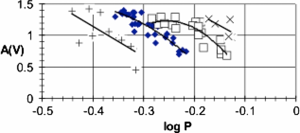
Figure 11. Position of a more extensive group of galactic field RR Lyrae data (65 stars) in the A(V) amplitude–log P diagram. Symbols, with the exception of the X's, are the same as in Figure 10. The X's are likely Oo III variables. They have large amplitudes for their periods. Note the presence of only one low-amplitude variable. Some of the low-lying points in the diagram (crosses) (log P > −0.35) may actually be Oo I Blazhko variables. Two or three of the Oo II stars at log P ∼ −0.28 and A(V) ∼ 1.2 mag may actually be Oo I variables instead of Oo II variables. Some of the other large amplitude stars may also be assigned to the wrong sequence.
Download figure:
Standard image High-resolution imageIt has been known for a long time that no short-period, metal-strong stars are found in galactic globular clusters, Smith (1995, p. 64). We carefully examined the Bailey diagrams of all the clusters studied in this investigation that might have stars falling in the same region of the AV, log P plane as the short-period, metal-strong stars in Figures 10 and 11. Although we found a number of stars that occupied the same region, they all failed to be fainter than the other stars in the clusters and are evidently just Blazhko stars or misclassified c variables, thus confirming the conclusion that they do not occur in galactic globular clusters.
The short-period variables are found not only in the galaxy but also in the LMC. We refer the reader to Figure 7 of Soszynski et al. (2009) where a group of RR Lyrae ab stars in the LMC occur in the V magnitude plot centered at log P ∼ −0.375 and V ∼ 19.67 mag. They are ∼0.3 mag fainter than the Oo I c variables centered at log P ∼ −0.5 and the Oo I ab variables centered at log P ∼ −0.3.
It is very important to note that the 12 Oo I stars form a well-defined sequence in Figure 10 yet have [Fe/H] values ranging from −0.55 to −1.57. Since the conventional wisdom is that the absolute magnitudes become more luminous as [Fe/H] decreases according to the equation ΔMV = 0.2 Δ[Fe/H], we would expect the more metal-poor stars to scatter over to near the three Oo II variables which is not the case. Clement & Shelton (1999a) concluded that the V amplitude for a given period is not a function of metal abundance, but rather a function of the Oosterhoff type. We concur and suggest that all of the variables within an Oosterhoff class, regardless of the [Fe/H] value, may have approximately the same mean absolute magnitude. Note the position of the three Oo II variables in Figure 10. Two variables have [Fe/H] near −1.6 (SU Dra [Fe/H] = −1.6, W Tuc [Fe/H] = −1.57). X Ari, the third star, for which [Fe/H] = −2.4, should be 0.16 mag brighter than SU Dra and W Tuc and displaced 0.055 in log P to a larger period if ΔMv = 0.2 [Fe/H] holds. Again, this is not the case. This implies that the mean magnitudes of the RR Lyrae stars may be sort of quantized, falling in four Mv groups, with few if any stars between the groups. The narrowest bands have σ's of ∼0.04–0.06 mag based on the scatter around the mean magnitude of some of the Oo I and II groups.
We now attempt to identify the minimum and maximum log P values of the four groups of RR Lyrae ab variables. We rely principally on the maximum and minimum log P values of individual stars observed within a group. The best estimates are given in Table 5.
Table 5. Log P values of Variables
| Group | log P | log P |
|---|---|---|
| (min) | (max) | |
| Shrt.Per. | −0.47 | −0.28 ? |
| Oo I | −0.35 | −0.175 |
| Oo II | −0.28 | −0.10 |
| Oo III | −0.24 | −0.02 |
Download table as: ASCIITypeset image
The log P (min) and log P (max) values must correspond closely to the log P values of the FBE and FRE of each group of RR Lyrae ab variables. Presumably, the temperatures of the four groups are similar at the FRE edge but increase in T at the FBE as we proceed from the Oo II variables to the short-period variables because the amplitudes increase at the edge. This is supported by the period–amplitude diagram (Figure 3) of Szczygiel et al. (2009) where the stars with log P < −0.35 (short-period group) exhibit the largest amplitudes. The maximum V amplitudes are ∼1.3 mag Oo II, ∼1.37 mag Oo I, and ∼1.43 mag short-period variables. With the aid of Equation (5), we find that the corresponding (〈B〉 − 〈V〉)0 values are 0.245 mag, 0.229 mag, and 0.216 mag. The temperatures corresponding to the color indices (according to Equation (3)) are 6970 K, 7050 K, and 7116 K. They indicate ∼70 K difference in temperature at the FBE between the Oo II and Oo I groups and ∼70 K difference between the Oo I and short period groups.
We emphasize that there are no small amplitude short-period variables in our samples to draw an accurate conclusion about the log P (max) value of the short-period variables. There is also no strong evidence that they form a tight, well-defined curve in a Bailey diagram. We also call attention to the variables in the two clusters, M3 and M62. Both are Oo I clusters with large numbers of RR Lyrae stars containing some Oo II-like variables. The Oo I ab variables in M3 ([Fe/H] = −1.5) extend from log P = −0.34 to log P = −0.175, while on the other hand, the Oo I ab variables in M62 ([Fe/H] = −1.18) extend from log P = −0.35 to log P = −0.185. The M62 variables appear to be shifted systematically to shorter periods by ∼0.01 in log P.
7. ABSOLUTE MAGNITUDES
Bono et al. (2007) provide a recent calibration of the absolute magnitudes of the RR Lyrae stars based on synthetic HB (SHB) simulations. They present, in their Table 2, the mean values of the HB type, RR Lyrae masses, absolute magnitudes, and pulsation parameters k(1.5)puls and k(2.0)puls of RR Lyrae models as a function of Z at a helium abundance of Y = 0.23. The numbers, shown in parentheses, of the pulsation parameters is the mixing-length parameters l/Hp, where l is the mixing length and Hp is the pressure scale height. Marconi et al. (2003) show that a mixing-length parameter of 2.0 is supported by the observational data of globular clusters. The observed maxima of the V light amplitudes (AV ∼ 1.2–1.3 mag), as well as the maxima light (B − V)0 ∼ 0.40 mag values in our data set of the variables in globular clusters, also support a value of 2.0 rather than 1.5 (see Marconi et al. 2003, Figures 4 and 5). We adopt the pulsation parameter, k(2.0)puls, in our calculations. We find that the following equations relate the mean absolute visual magnitude, 〈Mv(RR)〉, to the pulsation parameter k (2.0)puls as a function of the metallicity:


We have assumed [Fe/H] is given by [Fe/H] = log Z + 1.5 to insure [Fe/H] = −1.5 at Z = 0.001. According to Bono et al., the k(2.0)puls pulsation parameter is given by k(2.0)puls = 0.027 − log Pab − 0.142 AV.
We determined the log P values at five amplitude values (AV = 1.2, 1.0, 0.8, 0.6, and 0.4 mag) for each sequence and computed corresponding k(2.0)puls values. We adopted the average log P value and average k(2.0)puls value determined from the five amplitudes. For each Oo type, we present in Columns 2 and 3 (Table 6), the average log P and average k(2.0)puls values corresponding to each Oo type are given in Column 1. With the aid of the six equations above, we calculated the six 〈Mv〉 values for the corresponding Z values for each Oo type given in Columns 4–9. In addition, we adopted Mv = 0.55 mag for an Oo I star at Z = 0.001 and calculated the Mv values of the other sequences from their horizontal displacements (at AV = .7) from the Oo I sequence in the Bailey diagram, shown in the last column (10) of Table 6. The Mv values compare favorably with the corresponding values in Column 7 (Z = 0.001).
Table 6. Magnitudes Inferred from SHB Simulations
| Oo type | 〈log Pab〉 | 〈k(2.0)〉 | Z = 0.0001 〈Mv〉 | Z = 0.0003 〈Mv〉 | Z = 0.0006 〈Mv〉 | Z = 0.001 〈Mv〉 | Z = 0.003 〈Mv〉 | Z = 0.006 〈Mv〉 | Z = 0.001 〈Mv〉a |
|---|---|---|---|---|---|---|---|---|---|
| (mag) | (mag) | (mag) | (mag) | (mag) | (mag) | (mag) | |||
| met. strg. | −0.357 | 0.27 | 0.66 ± 0.01 | 0.77 ± 0.01 | 0.81 ± 0.01 | 0.83 ± 0.01 | 0.89 ± 0.01 | 0.91 ± 0.01 | 00.87 |
| Oo I | −0.235 | 0.149 | 0.47 ± 0.01 | 0.52 ± 0.01 | 0.53 ± 0.01 | 0.55 ± 0.01 | 0.59 ± 0.01 | 0.60 ± 0.01 | 00.55 |
| Oo II | −0.171 | 0.085 | 0.37 ± 0.01 | 0.38 ± 0.01 | 0.39 ± 0.01 | 0.40 ± 0.01 | 0.43 ± 0.02 | 0.44 ± 0.02 | 00.37 |
| Oo III | −0.099 | 0.012 | 0.25 ± 0.01 | 0.24 ± 0.01 | 0.22 ± 0.01 | 0.23 ± 0.01 | 0.25 ± 0.02 | 0.26 ± 0.01 | 00.23 |
Note. aThe absolute magnitude values in the last column have been calculated from displacements of other sequences from the Oo I sequence. Mv = 0.55 mag was adopted. Compare values with those in the other Z = 0.001 column (Column 7).
Download table as: ASCIITypeset image
The absolute magnitudes inferred from the SHB simulations exhibit a dependence on metallicity where we find little or no dependence within a sequence. We have adopted Mv values at the typical metallicities of the four sequences, which are given in Table 7.
Table 7. 〈MV〉 Values
| Oo type | Mv |
|---|---|
| (mag) | |
| Shrt. Per. | 0.91 |
| Oo I | 0.58 |
| Oo II | 0.40 |
| Oo III | 0.25 |
Download table as: ASCIITypeset image
We turn next to a discussion of the Clementini et al. (2003) study of RR Lyrae stars in fields A and B of the LMC. In Figure 12, we show the Bailey diagram of Field A. We identify a possible 14 more, certainly 12, Oo II variables (shown as squares) in the field. The average apparent 〈V〉 magnitude of the 12 Oo II stars is 19.32 ± 0.035 mag which compares with 〈V〉 = 19.44 ± 0.030 mag for 30 Oo I variables. The difference in magnitude of 0.12 mag compares with the difference of 0.18 mag based on the theoretical computations above. Metal abundances were determined by Clementini et al. (2003) from low-resolution spectra for about 80% of the variable stars. According to the authors, the [Fe/H] values are on the Harris (1996) scale which is equivalent to the Zinn & West (1984) scale. In Field A, we find [Fe/H] = −1.73 ± 0.06 for 8 Oo II variables and [Fe/H] = −1.44 ± 0.04 for 22 Oo I variables. Similar treatment of Field B yields 〈V〉 = 19.37 ± 0.03 mag (24 Oo I stars) and 〈V〉 = 19.18 ± 0.04 mag (5 Oo II stars). We find [Fe/H] = −1.82 ± 0.10 (4 stars) for Oo II variables and [Fe/H] = −1.49 ± 0.08 (11 stars) for the Oo I variables. The errors quoted are the errors in the mean values. Stars 19450 (log P = −0.400, AV = 1.344 mag 〈V〉 = 19.662 mag, [Fe/H] = −0.9) in Field A and 19037 (log P = −0.386, AV = 1.466 mag, 〈V〉 = 19.702 mag, [Fe/H] = −1.26) in Field B would both be classified as belonging to the short-period sequence of stars based on their amplitudes and periods. Each is considerably fainter than the mean values of the Oo I stars in their fields, and each is among the most metal-strong variables sampled in their fields. On average, they are 0.28 mag fainter than the Oo I variables and differ by ∼0.02–0.04 in [Fe/H] from the Oo I variables. These two stars, as well as the difference in magnitudes between the Oo I and Oo II variables, are good examples of the breakdown of trying to use any existing MV = f ([Fe/H]) relation to estimate absolute magnitudes of RR Lyrae variables.

Figure 12. RR Lyrae ab variables in Field A of the LMC plotted in the AV–log P diagram (Bailey diagram). The majority of the stars are Oo I (solid diamonds), but there is also a significant population of Oo II variables (open squares). As in all other populations where it is possible to distinguish the two Oo types, the average magnitude of the Oo II variables is brighter than the average magnitude of the Oo I variables. The data point at log P = −0.40 is actually a short-period variable and is 0.22 mag fainter than the mean magnitude of the Oo I variables.
Download figure:
Standard image High-resolution imageTo obtain accurate distances, accurate reddening values are required. Two sets of reddening values are available for the two fields besides the entries in Table 3. Clementini et al. (2003) estimated the reddening in the two fields based on the Sturch method and from the colors of the edges of the instability strip. They found E (B − V) = 0.116 ± 0.017 mag (Field A) and 0.086 ± 0.017 mag (Field B), respectively. McNamara (2011) found 0.114 ± 0.004 mag for Field A and E (B − V) = 0.091 ± 0.005 mag for Field B by methods similar to those described in this paper. We find (Table 3) Field A, E (B − V) = 0.102 ± 0.002 mag and Field B, E (B − V) = 0.078 ± .002 mag. We give double weight to the latter two values and find the average reddening to be: Field A, E (B − V) = 0.109 ± 0.004 mag and Field B, E (B − V) = 0.083 ± 0.003 mag. If we assume the absorption of light in the V band, AV is given by AV = 3.1 E (B − V), and if we adopt the 〈V〉 values above, we find the average reddening-free magnitudes, given in Table 8.
Table 8. 〈V〉0 Values of Variables in the LMC
| Field A | Field B | |
|---|---|---|
| Oo I | 19.10 | 19.11 |
| Oo II | 18.98 | 18.92 |
Download table as: ASCIITypeset image
We adopt Mv = 0.58 mag for the Oo I stars and Mv = 0.40 mag for the Oo II variables. The distance moduli of the LMC become 〈V〉 − Mv = 18.52 mag for the Oo I stars and 18.56 mag for the Oo II stars. The weighted mean is 18.53 ± 0.02 mag.
To investigate the dependence of Mv on [Fe/H], we found the dependence of the mean intensity V magnitudes, 〈V〉, of the stars with available [Fe/H] data. With the aid of regression analysis, we found the following expressions where n is the number of stars.

The coefficients of the [Fe/H] term are all small or even negative which suggests that the usual expression, ΔMv = 0.20 Δ[Fe/H], is not valid within an Oo type. Unfortunately, because of the depth of the galaxy, a large amount of scatter is introduced into the 〈V〉 date resulting in large errors in the [Fe/H] term, so we cannot be certain of this conclusion. We will revisit this issue later where the data are more certain supporting this conclusion.
Walker (2012) has recently discussed the distance modulus of the LMC utilizing five different distance indicators. He finds a mean value of (V − Mv)0 = 18.48 mag with a 3% uncertainty. This distance modulus suggests the absolute magnitudes of Mv = 0.58 mag (Oo I stars) and Mv = 0.40 mag (Oo II stars) are a little too bright and should more appropriately be Mv ≈ 0.63 mag (Oo I stars) and Mv ≈ 0.48 (Oo II stars).
An even more recent very accurate distance to the LMC of D = 49.97 ± 0.19 kpc, corresponding to (V − Mv)0 = 18.49 ± 0.01 mag, has been determined from the analysis of eight LMC eclipsing binaries (Pietrzynski et al. 2013). The Clementini et al Oo I magnitudes above 19.10 mag, in combination with this distance modulus, yield Mv = 0.61 ± 0.03 mag for the Oo I variables.
The luminosity (Mv value) of the Oo I variables is a very important issue, since they are by far the most abundant RR Lyrae ab stars in galaxies exhibiting both population I and II stars. We have attempted to estimate an independent Mv value by appealing to the SX Phe stars in M3. Cohen & Sarajedini (2012) list 11 SX Phe stars in M3. Their position in a 〈V〉, log P diagram is shown in Figure 13. A least-square fit to the fundamental pulsators (small solid diamonds) is 〈V〉 = −2.655 (±0.408) log P + 14.395 (±0.567), σ = 0.11 mag. The three other stars (open squares) are evidently second-overtone pulsators. At log P = −1.42, where most of the data points are centered, 〈V〉 = 18.16 ± 0.04 mag. The P–L relation (Mv = −2.90 log P − 1.27 − 0.19 [Fe/H], σ = ± 0.02 mag) McNamara (2011) gives Mv = 3.13 ± 0.02 mag. at log P = −1.42 and [Fe/H] = −1.5. Since 〈V〉 = 15.64 mag for the Oo I stars in M3, this implies their 〈Mv〉 value is 〈Mv〉 = 0.61 ± 0.04 mag.
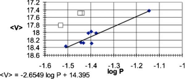
Figure 13. Period–luminosity relation of SX Phe stars in M3. The solid diamonds are the fundamental pulsating stars and the open squares are second-overtone pulsating variables. The equation in the panel is the fit to the fundamental pulsating variables.
Download figure:
Standard image High-resolution imageIn addition, we have attempted to determine the Mv value from fundamental considerations. We have utilized the period–radius and period–temperature (static stars) relations discussed previously in the text in connection with the equation L/L☉ = (R/R☉)2 (T/T☉)4 to express the bolometric magnitude of the variables as a function of period. Again, we adopt M(bol)☉ = 4.75 and T☉ = 5780 K. We find Mbol = −0.379 (±0.019) log P + 0.434 (±0.005), σ = ±0.003. If we average over the log P interval of Oo I variables (−0.34 to −0.175), the Castelli (1998) bolometric corrections given in CCC indicate Mv = 0.56 mag, while the bolometric corrections in the Lejeune et al. (1998) tables yield Mv = 0.60 mag. To correct to intensity mean values (Marconi et al. 2003), we add 0.01 mag and find 〈Mv〉 = 0.57 mag and 〈Mv〉 = 0.61 mag. If we average the six Mv values (0.57 mag, 0.58 mag, 0.61 mag, 0.61 mag, 0.61 mag, 0.63 mag) of the Oo I variables, giving double weight to the Walker (2012) and Pietrzynski et al. (2013) values, we find 〈Mv〉 = 0.61 ± 0.02 mag, where we estimate the error to realistically be σ = 0.02 mag instead of the statistical error of 0.01 mag. All of the Mv values lie within 2σ of the mean value. Since the Oo II stars are brighter by 0.18 ± 0.02 mag than Oo I stars, this implies the best average Mv value for the O II variables is 〈Mv〉 = 0.43 ± 0.03 mag.
The 〈V〉 intensity means are available for 17,693 ab variables in the Ogle III catalog of variable stars of the LMC. In what follows, we have attempted to calculate the average apparent magnitudes of the four sequences. We arbitrarily restrict our sample of stars to 〈(V) − (I)〉 values >0.00 mag, and 〈V〉 magnitudes between 18.90 mag and 19.90 mag to eliminate foreground and background stars and eliminated a few stars with excessive large colors, 〈(V) − (I)〉 values >1.00 mag. Periods have been used to designate the four sequences: short-period variables −0.43 ⩽ log P ⩽ −0.35, Oo I variables −0.3 ⩽ log P ⩽ −0.25, O II variables −0.175 ⩽ log P ⩽ −0.09, and Oo III variables −0.089 ⩽ log P ⩽ 0.0. Not all stars in a sequence are included because of unknown overlapping of sequences at certain periods. The period intervals were chosen where a group is dominant. The Oo type, log P interval, number of variables, and 〈V〉 magnitudes are given in the first, second, third, and fourth columns of Table 9, respectively. The V magnitudes show, as above, an increase in luminosity proceeding from the short-period stars to the Oo III variables.
Table 9. Magnitudes of RR Lyrae Stars (LMC)
| Type | log P | n | 〈V〉 mag | 〈[Fe/H]zw〉 | (Mv)aa | (Mv)da | %b | % Galaxy |
|---|---|---|---|---|---|---|---|---|
| Short Per | −0.47 to −0.35 | 233 | 19.63 ± 0.01 | −1.01 ± 0.02 | 0.81 | 0.89 | 3 | 14 |
| Oo I | −0.30 to −0.25 | 6593 | 19.43 ± 0.00 | −1.51 ± 0.00 | 0.61 | 0.61 | 82 | 66 |
| Oo II | −0.175 to −0.09 | 1282 | 19.28 ± 0.01 | −1.64 ± 0.01 | 0.46 | 0.43 | 14 | 15 |
| Oo III | −0.09 to 0.00 | 70 | 19.17 ± 0.02 | −1.80 ± 0.02 | 0.35 | 0.29 | 1 | 5 |
Notes. aThe absolute magnitude of the Oo I variables is assumed to be 0.61 in Columns 6 and 7. The (Mv)a values of the other sequences (types) are found from 〈V〉 values in Column 4. The (Mv)d values in Column 7 are found from horizontal displacements of other sequences relative to the Oo I variables in Bailey diagrams. bThe numbers in Column 3 have been modified to find the %'s in this column.
Download table as: ASCIITypeset image
In Column 5, (Mv)a, of Table 9, we have arbitrarily set the absolute V magnitude of the Oo I variables at 0.61 mag; the absolute magnitudes of the other three groups follow from the differences of the 〈V〉 magnitudes in Column 4. In Column 6, (Mv)d, of Table 9, we adopted 0.61 mag for the Oo I variables and calculated the Mv values of the other sequences from the horizontal displacements (at AV = 0.7) of the various sequences in the Bailey diagram. An error of 0.01 in the displacement along the log P axis corresponds to an error of 0.03 mag in Mv. The two methods predict 〈Mv〉 = 0.43 mag and 0.46 mag for the Oo II stars. A relatively small number of stars are involved in the determination of the 〈V〉 magnitudes of the stars of the short period and Oo III sequences, but the values found from the two methods differ only by 0.06 mag and 0.08 mag. The percentages of stars in each group given in the next to last column are very rough. They were obtained by doubling the numbers in Column 3 of short-period, Oo II, and Oo III stars. The remaining stars were all assumed to be Oo I stars. The data are accurate enough to show that the vast majority of variables are Oo I and II (∼96%), and there are between five and six Oo I variables for every O II variable in the LMC.
The mean 〈[Fe/H]ZW〉 values (Column 5) for each group, based on the Zinn & West (1984) system, were determined from the Fourier parameter φ31 (Equations (3) and (4) of Pietrukowicz et al. 2012). The equations are also found in earlier papers by Smolec (2005) and Papadakis et al. (2000). The values compare favorably with the average [Fe/H] values in Fields A and B discussed above (Clementini et al. 2003).
In addition, we have attempted to estimate the percentages of the groups in the galaxy from the right panel of Figure 2 found in Szczygiel et al. (2009). Their figure shows the pulsation periods of 1423 RR Lyrae ab variables within 4000 parsecs of the Sun from the All Sky Automated Survey (ASAS). The areas under the curve were measured at the appropriate periods and some adjustments made for overlapping periods. The very rough values are presented in the last column of Table 9. The increase percentages of the short-period variables and Oo III variables over the percentages in the LMC are probably real in light of the ease we picked up these variables in the small galactic samples we discussed in Section 6.
A very careful perusal of Figure 7 in the Soszynski et al. (2009) paper on RR Lyrae stars in the LMC reveals discontinuities (at log P ∼ −0.35 separating the short period variables from the Oo I variables and log P ∼ 0.18 separating the Oo I variables from the Oo II variables) in the period–luminosity diagram of V mag versus log P (upper panel). A clump of data points of ab variables at log P < −0.35 is evident at V ∼ 19.7 mag (the short-period RR Lyrae stars); the ab variables in the log P interval −0.34 < log P < −0.18 are primarily the Oo I ab variables at V ∼ 19.4 mag and have magnitudes similar to the RR Lyrae c variables in the log P interval −0.55 < log P < −0.47. The Oo II variables at V ∼ 19.2 mag, dominate in the log P interval −0.175 < log P < −0.10. A few Oo III stars are evident at log P > −0.10 at V ∼ 19.05 mag. Note also that the RRc variables in the log P interval −0.43 < log P < −0.35 have V magnitudes of V ∼ 19.2 mag, brighter by ∼0.2 mag than the shorter period RRc variables in the log P interval −0.55 < log P < −0.47. They must be the Oo II c variables. There are overlaps of periods (see Section 6) of the groups. The periods or period intervals described above are where various groups dominate.
No convincing evidence of discontinuities is present in either the I mag versus log P or the Wi versus log P diagrams (Wi is the Wessenheit index); bottom two panels of their Figure 7. The reason can be traced to the fact that the individual groups obey P–L relations very similar to the P–L relation obtained by fitting them together. Only in the V band are the 〈V〉 magnitudes of each group flat independent of period. The exception may be, as we pointed out previously, the Oo II variables that exhibit a small increase (∼0.15 mag) from the shortest to the longest period variables. No clean, well-defined separations of the RR Lyrae ab variables groups are evident in Bailey diagrams of the variables in large surveys such as OGLE.
8. SOME COMMENTS ON OOSTERHOFF I AND II VARIABLES
In the first panel of Figure 14, we plot the 〈V〉 magnitudes of the Oo II-like stars (evolved stars) in M3 as a function of log P. The line which fits the data is essentially flat with a small positive slope. The two lower panels are similar diagrams of variables in two Oo II clusters (NGC 5466 and NGC 5053) in which only Oo II variables are present. Similar diagrams in which the 〈B〉 magnitudes are plotted instead of 〈V〉 are shown in Figure 15. The stars in M3 now exhibit a significant positive slope where the stars in NGC 5466 and NGC 5053 exhibit negative slopes, but smaller negative slopes than in the V band. In spite of the fact that the evolved stars in M3 are about as bright as Oo II variables and have similar periods as Oo II variables, they are not strictly identical to Oo II variables. Cacciari et al (2005) probably made a good decision in referring to these over-luminous variables in M3 as evolved variables rather than Oo II variables. This is the reason we have referred to these variables as Oo II-like rather than as Oo II variables.
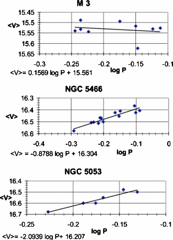
Figure 14. Plots of the 〈V〉 magnitude vs. log P (days) of RR Lyrae ab variable stars in three globular clusters. The upper panel is the Oo II-like evolved variables in M3. The fit to the data points is essentially flat. The variable stars in the two Oo II clusters NGC 5466 and NGC 5053 both exhibit weak period–luminosity relations.
Download figure:
Standard image High-resolution image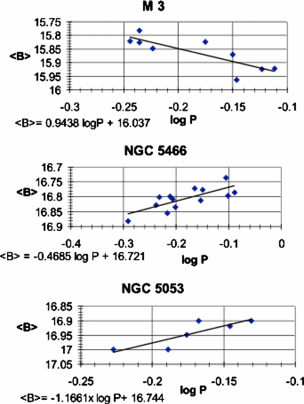
Figure 15. Plots of the 〈B〉 band magnitudes vs. log P (days) of RR ab Lyrae stars in three globular clusters. The upper panel is the Oo II-like evolved variables in the Oo I cluster M3 which exhibit a positive slope. The variables in the two Oo II clusters NGC 5466 and NGC 5053 both exhibit weak period–luminosity relations with negative slopes.
Download figure:
Standard image High-resolution imageIn order to examine this issue further, we calculated the slopes of the AV–log P and 〈V〉–log P relations in each cluster. We assume the distribution of stars in a Bailey diagram is linear, even though it is quadratic as the M3 plots shows because, in many clusters, not enough variables are present to reveal the true nature of the curves. The results are found in Table 10 where the clusters are identified in Column 1 and Oo type given in Column 2; the Oo I clusters are tabulated at the top of the table and Oo II clusters at the middle. Slopes and slope errors of the AV–log P and 〈V〉–log P relations are given in Columns 3 and 4, respectively. It is evident that both the Oo I stars and Oo II-like variables in the Oo I clusters exhibit steeper (–) slopes in the AV–log P diagrams than the slopes of the stars in Oo II clusters. Compare the average values −6.55 Oo I, −6.0 Oo II-like variables with −3.88 for the Oo II stars. If M68 and NGC 5053, which have unusually small negative slopes (probably due to the presence of Blazhko variables), are removed from the Oo II sample, the average slope of the Oo II clusters is −4.59 ± 0.46, still a smaller negative slope than the Oo I clusters.
Table 10. Slopes of the AV–log P and 〈V〉–log P Relations
| Cluster | Type | AV − log P | 〈V〉 − log P | log P At AV = 0.8 |
|---|---|---|---|---|
| (m) | (m) | |||
| M3 | Oo I | −6.02 ± 0.42 | −0.34 ± 0.16 | −0.23 |
| Oo II | −7.26 ± 0.82 | 0.16 ± 0.28 | −0.165 | |
| M5 | Oo I | −5.93 ± 0.41 | −0.85 ± 1.98 | −0.23 |
| M62 | Oo I | −5.55 ± 0.38 | −0.94 ± 0.60 | −0.235 |
| Oo II | −4.73 ± 0.72 | 0.49 ± 1.18 | −0.175 | |
| M54 | Oo I | −7.02 ± 0.85 | 0.26 ± 0.50 | −0.232 |
| M75 | Oo I | −7.96 ± 2.30 | 0.89 ± 1.01 | −0.24 |
| NGC 1851 | Oo I | −4.94 ± 1.49 | −0.04 ± 0.73 | −0.21 |
| NGC 3201 | Oo I | −5.47 ± 0.75 | 0.03 ± 0.32 | −0.22 |
| Rup 106 | Oo I | −9.49 ± 1.16 | 0.39 ± 0.61 | −0.225 |
| Avg | Oo I | −6.55 ± 0.54 | −0.07 ± 0.22 | −0.228 ± 0.003 |
| Avg | Oo II-like | −6.0 ± 1.26 | 0.32 ± 0.17 | −0.170 ± 0.005 |
| M68 | Oo II | −0.91 ± 1.44 | −0.75 ± 0.34 | −0.165 |
| NGC 5053 | Oo II | −1.92 ± 3.87 | −20.09 ± 0.30 | −0.17 |
| NGC 5286 | Oo II | −5.69 ± 0.86 | −1.28 ± 1.14 | −0.18 |
| NGC 5466 | Oo II | −5.50 ± 0.86 | −0.88 ± 0.11 | −0.17 |
| M92 | Oo II | −3.45 ± 3.68 | −0.44 ± 0.65 | −0.165 |
| M55 | Oo II | −6.21 ± 2.16 | −0.48 ± 1.02 | −0.16 |
| M15 | Oo II | −3.08 ± 0.76 | −0.75 ± 0.35 | −0.165 |
| M2 | Oo II | −4.30 ± 0.68 | −0.36 ± 0.37 | −0.15 |
| Avg | Oo II | −3.88 ± 0.63 | −0.88 ± 0.19 | −0.166 ± 0.003 |
Download table as: ASCIITypeset image
The slopes of the 〈V〉–log P relations for the variables in Oo I clusters alternate between small negative and positive slopes. The average value, −0.07 ± 0.22, is essentially zero indicating that the Oo I stars in clusters on average have the same 〈V〉 magnitudes. On the other hand, all of the Oo II variables in clusters exhibit small negative slopes indicating that the long-period variables are more luminous than the shorter-period variables. At the average slope, −0.88 ± 0.19, and log P interval (−0.28 to −0.10), corresponds to an increase of 0.16 ± 0.03 mag in 〈V〉 across the RRab instability strip. The Oo II-like variables (in only 2 clusters, a small sample) give a small positive slope (0.32 ± 0.17) indicating that the shorter-period variables may be slightly more luminous than the longer-period variables.
In many cases in the analysis above, the clusters have few variables, and frequently, the errors in the slope are equal if not larger than the slopes. In an ideal case, one would like to have a large number of variables at all periods of a sequence and this condition is not fulfilled.
Our analysis is very similar to plotting the AV amplitudes of the variables versus their log P values (Bailey diagrams) and defining lines (which are approximations) to separate the Oo I and Oo II groups (Clement & Shelton 1999a). By utilizing the log P values at AV = 0.80 mag and average slopes (we eliminated the slopes inferred from the variables of the two Oo II clusters M68 and NGC 5053 in calculating the average slope of the Oo II relation), we find the following equations:


The errors in the average slopes are ∼0.48 and n is the number of clusters. The slope (absolute value) of the Oo II AV–log P relation must be considerably smaller than the slope of the Oo I AV-log P relation in order for the 〈V〉 magnitudes of Oo I variables to be independent of period and the Oo II variables to exhibit a P–L relation (longer-period stars being brighter).
In the Bailey diagram (Figure 16), we again plot the M3 data, solid diamonds Oo I stars, Oo II-like variables open squares. The X's are the Oo III variables in the globular cluster NGC 6441 (Pritzl et al. 2002) and the solid curve to the right is the least-square fit to the data points. The solid triangles are the four Oo III variables discussed in Section 5, and the three plus signs are short-period, metal-strong variables. The thin curve on the extreme left, fitting the three short-period metal-strong variables, is a theoretical curve (−2.90 log P − 0.240 AV2 − 0.133 AV = constant) insuring that every point along the curve has the same V magnitude. The constant is arbitrary, and any value can be chosen to slide the curve to any log P value along the horizontal axis. The equation was derived by insisting that the Mv value be constant insuring that V must also be constant, and utilizing the P–T, P–R, and P–AV relations alluded to earlier in our discussion.
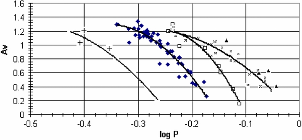
Figure 16. RR Lyrae ab variables from several star populations plotted in an AV–log P diagram. As in previous diagrams the solid diamonds and open squares are the M3 Oo I and Oo II-like stars and the corresponding curves, fitting the points, mark the regions where Oo I and Oo II variables are invariably found. The X's are the Oo III stars of the metal-rich cluster NGC 6442. The solid triangles are the Oo III stars found in other clusters discussed in the text. The curve fitting the Oo III variables is based only on the NGC 6442 variables. The crosses are three short-period variables found in the galactic field. The thin curve fit to the short-period variables is a theoretical curve that predicts the same V magnitude for any point along the curve, and can be placed at any position along the log P axis. Note that all the curves in the diagram are very similar to the theoretical curve, although the Oo III curve is somewhat flatter. If we assume the average absolute magnitude of the Oo I stars is 0.61 mag, the horizontal displacement of the other curves at AV = 0.7 mag indicates the other absolute magnitudes are: short-period variables Mv = 0.92 mag, Oo II stars Mv = 0.42 mag, and Oo III stars Mv = 0.29 mag.
Download figure:
Standard image High-resolution imageWe note that the M3 curves both resemble the theoretical curve, while the NGC 6441 curve is a little flatter. If the theoretical curve is fit with a linear relation, the slope is −6.04 ± 0.46, consistent with the average slope of the Oo I clusters in Table 10.
The four new Oo III variables (solid triangles) are displaced to longer periods relative to the variables of the metal-strong cluster NGC 6441 (crosses). If real (the sample is small), their displacement indicates that they are ∼0.03 mag brighter than the NGC 6441 variables. This suggests (contrary to our arguments concerning other groups) that there may be a very weak dependence of Mv on [Fe/H] for the Oo III group.
In the last column of Table 10, we list the log P values at AV = 0.80 mag inferred from Bailey diagrams of nearly all the galactic globular clusters. The estimated uncertainty in determining this value is ∼0.01 in some of the clusters with sparse data. The average value of the Oo I clusters is −0.229 ± 0.003, and the average value of the Oo II-like variables in Oo I clusters is −0.170 ± 0.005, and strictly Oo II clusters is −0.166 ± 0.003. Since the stars have identical temperatures at this AV amplitude, and ΔMv = −2.90Δ log P, it follows that the Oo II ab variables are 0.18 mag more luminous than the Oo I variables, in agreement with our previous estimates. Since the Oo II variables exhibit a P–L relation (the stars of long period (small amplitude) are ∼0.15 mag brighter than the stars of short period (large amplitude)), the difference can vary with period or AV amplitude. The 0.18 mag is a good average value. Note that the largest residual in log P is 0.02 at about 2σ the estimated error. Since a point in the AV–log P diagram presumably has the same temperature and radius, we consider the data in the last column of Table 10 as corroboratory evidence that the variables within an Oo class (at least Oo I and II) have about the same average Mv values (the Oo II clusters showing a P–L relation) regardless of the variation of [Fe/H] within the class, in agreement with other evidence we have presented.
Finally, we turn to ω Cen (Rey et al. 2000) and plot the 〈V〉 magnitudes of Oo I, II, and possible III RR Lyrae ab variables against their [Fe/H]hk values in the upper panel Figure 17 and against log P in the lower panel. The same plots are given for the RR Lyrae c variables of ω Cen in Figure 18. Data are found in Table 5 of Rey et al. (2000). We have assigned the stars to either Oo I or Oo II strictly on the basis of their [Fe/H]hk values except at the transitions ([Fe/H]hk ∼ −1.5 ab, ∼−1.25 c, where 〈V〉 magnitudes proved useful as a discriminate.
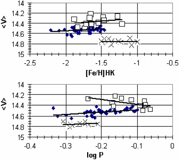
Figure 17. RR Lyrae ab variables in ω Cen. The upper panel gives the dependency of 〈V〉 on [Fe/H]hk. The lower panel gives the dependency of 〈V〉 on log P. The X's are Oo I variables, solid diamonds Oo II variables, and open squares likely Oo III variables.
Download figure:
Standard image High-resolution image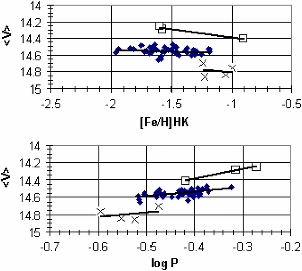
Figure 18. RR Lyrae c variables in ω Cen. Symbols and plots are similar to Figure 17.
Download figure:
Standard image High-resolution image
The assignment of some of the variables to the Oo III category is questionable. Five stars were assigned to this category simply because their log P values are > −0.10. The Oo II variables are normally restricted to log P values in the interval −0.28 to −0.10. Three Oo II variables have log P values <−0.28, and so there may be variables that exceed log P = −0.10. This view is supported by the 〈V〉–log P plot in Figure 17 where at least four Oo III variables seem to lie on an extension of the P–L relation of the Oo II relation. These are the same four variables that fall nearest to the Oo II P–[Fe/H]hk line in the upper panel. The other variables were assigned Oo III status based on their displacement above the Oo II stars. In all cases, their log P values are >−0.24.
The important issue is the dependence of 〈V〉 on [Fe/H]. The answer is provided by the following four equations:
In each case, the error in the slope is comparable to the small slope values that alternate in sign. The average slope is = −0.024 ± 0.039. If we neglect the Oo III group, because the assignment of some of the stars to this category is suspect, we find the average slope is −0.002 ± 0.041. In either case, it is apparent that the 〈V〉 magnitudes are independent of [Fe/H] in agreement with supporting data presented previously. The fits of Equations (26), (27), and (28) to the ab variables can be seen in Figure 17 and the fit of Equation (29) to the c variables is shown in Figure 18.
Weak period–luminosity relations are evident for both the RR Lyrae Oo II ab (Figure 17) and Oo II c (Figure 18) variables in ω Cen. The equations representing the data are:
A summary of the mean 〈V〉 magnitudes, mean periods, and mean [Fe/H]hk values of the Oo groups is given in Table 11, where n is the number of stars. We only used seven stars that we are reasonably confident are Oo III ab variables in defining the mean value.
Table 11. RR Lyrae Stars ω Cen
| Group | 〈V〉 | 〈P〉 | 〈[Fe/H]hk〉 | n |
|---|---|---|---|---|
| (mag) | (days) | |||
| Oo I | ||||
| ab | 14.75 ± 0.01 | 0.54 | −1.3 | 12 |
| c | 14.79 ± 0.04 | 0.29 | −1.13 | 4 |
| Oo II | ||||
| ab | 14.51 ± 0.01 | 0.64 | −1.76 | 40 |
| c | 14.55 ± 0.01 | 0.38 | −1.53 | 41 |
| Oo III | ||||
| ab | 14.31 ± 0.02 | 0.71 | −1.51 | 7 |
| c | 14.32 ± 0.05 | 0.47 | −1.36 | 3 |
Download table as: ASCIITypeset image
The weighted mean 〈V〉 magnitude (14.76 mag) of the Oo I variables combined with Mv = 0.61 mag leads to an apparent distance modulus of 〈V〉 − Mv = 14.15 mag. Color excess values of 0.12 mag (Harris 1996 (2010 edition)), 0.136 mag (Schlegel et al. 1998), 0.17 mag (McNamara 2011), and 0.15 mag, found from fitting the color–magnitude diagram (B − V) value "turn off" of the earliest and dominant stellar population in ω Cen to reddening-free "turn offs" of globular clusters with the same [Fe/H] value (−1.7), lead to an average value of E (B − V) = 0.144 ± 0.01 mag. We assume AV = 3.1 E (B − V)and find a true distance modulus of 13.70 ± 0.05 mag. The major contributor to the uncertainty is the ± 0.03 mag in AV. The true distance modulus found here may be compared with 13.62 ± 0.05 mag (becomes 13.67 ± 0.05 mag if the same color excess is used) found from SX Phe stars (McNamara 2011), and 13.70 mag (Del Principe et al. 2006) found from infrared magnitudes of RR Lyrae stars.
We need to emphasize that the ∼0.20 mag difference between the Oo II and Oo I variables (the Oo II stars being brighter) can be found in the RR Lyrae star literature over the last 50 yr. As we already pointed out, Sandage (1958) was the first to point out this possibility. This topic was pursued vigorously in the 1980s to late 1990s. SHB models, based on stellar-evolutionary tracks, indicated that the Oo II variables are highly evolved stars, probably many from the blue HB, evolving to lower temperatures through the instability strip at higher luminosities than the Oo I variables that tend to be located at lower luminosities near the zero-age HB. See Lee (1991) for an early summary. Recent studies of the age–metallicity relation (AMR), by Marin-Franch et al. (2009) and Dotter et al. (2011) of galactic globular clusters (GGC), indicate that for clusters <8 kpc from the galactic center, the Oo II clusters ([Fe/H] < −1.5) on average are older than the Oo I clusters ([Fe/H] > −1.5) by ∼0.5 Gyr (∼13.2 Gyr versus ∼12.7 Gyr). A hint of this difference is evident in an earlier study (Figure 1) by McNamara et al. (2004). At larger distances from the galactic center, many GGC appear to be younger by up to as much as 5 Gyr, and most of the youngest are Oo I globular clusters.
We note that the Oo III variables that we have identified are found in both Oo I and Oo II GGC as well as in the LMC and galaxy. These RR Lyrae stars are the most luminous. Why they are more luminous obviously, must be related somehow, to their evolution status but the somehow remains a mystery.
The evolutionary track (redward) of a single-mass star through the RR Lyrae ab instability strip indicates an increase of ∼0.15 mag in M(bol) (Lee 1991), which translates to ∼0.02–0.03 mag in Mv. Since the Mv values of the Oo II-like variables in globular clusters are essentially independent of period and B − V, a single mass value is probably appropriate for all of the Oo-like stars. On the other hand, in the strictly Oo II clusters, variables in the V band exhibit a weak P–L relation. An increase of ∼0.15 mag from the short-period variables (log P ∼ −0.28) to the long-period variables (log P ∼ −0.10). This implies a single mass value may not be appropriate for all of the Oo II variables in the instability strip.
9. THE OOSTERHOFF-INTERMEDIATE CLUSTERS (LMC)
The Oosterhoff groups are defined by the average periods of the RR Lyrae ab variables. Oo I clusters have average periods of 〈Pab〉 < 0.58 days, and Oo clusters have average periods of 〈Pab〉 > 0.62 days. Some globular clusters in the LMC and dwarf spheroidal galaxies of the local group have RR Lyrae ab variables that have 〈Pab〉 values which fall in between these limits and are called intermediate clusters (Oo int). The reader is referred to two recent papers and references therein (Kuehn et al. 2011, 2012) for extensive discussions of these intermediate systems.
We have analyzed the RR Lyrae star data in five LMC globular clusters some of which are classified as Oo int. GL 0435 (Reticulum) which has an average P value, 〈P〉 = 0.553 days, and appears to be a normal Oo I cluster, although [Fe/H] = −1.7. NGC 1466 (〈P〉 = 0.587 days) is unusual in three respects. Although it appears primarily to be an Oo I cluster, there are no variables with log P values smaller than log P = −0.30 days, two stars slightly exceed the limit of log P = −0.175 days of galactic Oo I clusters, and the metallicity, [Fe/H] = −1.85 is considerably smaller than what is normally found in Oo I galactic globular clusters. NGC 1835 (〈P〉 = 0.583 days) shows a large scatter in the 〈V〉 magnitudes (∼.8 mag) of the variables and may be mixed with some LMC variables. The (〈B〉 − 〈V〉)0 color indices indicate it is primarily an Oo II cluster. Only three stars exceed log P = −0.20. NGC 2257 (〈P〉 = 0.608 days) shows Oo II characteristics. It contains six variables with log P < −0.28, the usual cut off of Oo II variables in galactic globular clusters. If these six stars are eliminated, the average period becomes 〈P〉 = 0.643 days, and the cluster would be classified as Oo II instead of Oo int based on its average period.
In summary, the Oo int clusters take on either Oo I or Oo II characteristics and do not show a mix of the two classes in our limited sample. The unusual average periods appear to be due to an unusual distribution of periods. The shorter period variables are missing in the more metal-poor clusters, and two of the clusters that exhibit Oo I characteristics have unusually low metallicities when compared to galactic globular Oo I clusters.
10. CONCLUSIONS
We have derived a set of equations that can be used to derive the intrinsic-color indices of RR Lyrae variables from their light amplitudes. In combination with the observed color indices, very accurate color excess values can be derived. We discuss the influence of Blazhko variables on color excess determinations and conclude that they yield good values as long as they are near maximum amplitude in their Blazhko cycle or have amplitudes >0.90 mag in V. The reddening, E (B − V), determined for 18 globular clusters by our equations are compared with the reddening determined by others and found to always agree on average to less than 0.01 mag.
We discuss the presence of Oo II-like variables in three Oo I globular clusters. Their position in AV–log P diagrams is similar to the Oo II stars; their luminosities and periods resemble the Oo II variables. The Oo II variables, however, exhibit a weak period–luminosity relation in the V band, but the Oo II-like variables in Oo I clusters fail to do so.
Four new Oo III variables, two found in metal-weak clusters, are discussed and found to be ∼0.2 mag brighter than typical Oo II variables.
Galactic field variables are discussed from the point of view of their position in the AV–log P diagrams. The majority of these variables are Oo I or Oo II, but a small minority of short-period, metal-strong variables are clearly delineated in a Bailey (AV–log P) diagram. They are ∼0.30 mag fainter than the Oo I variables. There is also some evidence for Oo III variables in the galactic field.
The RR Lyrae ab variables are found to occupy four regions of a Bailey diagram and consequently appear to be restricted to four sequences or groups. The groups in order of increasing period and luminosity are: the short-period metal-strong variables, Oo I variables which are by far the most prevalent, Oo II variables, and the very rare Oo III variables. Although the average [Fe/H] values differ from group to group, we find no hard evidence that the luminosity of the variables within a group depends on the [Fe/H] value. In fact, just the opposite appears to be the case, contrary to the prevailing view.
The best approach in using RR Lyrae ab variables to find a distance to a field where both O I and Oo II stars are present, is to first plot all the variables in a Bailey diagram (AV verses log P) to identify which variables are Oo I a or Oo II. A typical separation of ∼0.06 days in log P in the steepest parts of the curves should be evident. The mean Mv values in combination with the 〈V〉 values of each group and the reddening inferred from the amplitudes of the light variations should yield the distance.
The mean Mv value of the Oo I group is very important since the mean absolute magnitudes of the other groups can be inferred from their displacements from the Oo I stars in Bailey diagrams. The best value at present is Mv = 0.61 ± 0.02 mag and certainly is subject to improvement. For strictly Oo II clusters, Mv = 0.43 ± 0.03 mag. This value is subject to more uncertainty because of a weak P–L relation for the Oo II group.
The intermediate LMC globular clusters (Oo int) in our limited sample have either Oo I or Oo II variables. The variables have a peculiar distribution of periods, that when averaged, leads to unusual average periods not found generally among the galactic globular clusters. Two clusters with Oo I variables have [Fe/H] values <−1.55 where Oo I variables usually transition to Oo II variables in galactic globular clusters.
We would like to thank an anonymous referee for a careful review and very useful comments.