


ABSTRACT
We report the results of a study of multicolor optical microvariability in the Blazar S5 0716+714. S5 0716+714 was observed in the B and I bands continuously for five consecutive nights in 2003 March. This is the first study to apply color analysis, structure function, and cross-correlation analysis on an optical data set with the temporal coverage and photometric quality that characterizes this data. The source displayed variability on timescales from days to tens of minutes in both bands. Discrete events in the light curves lead to the determination of a range in the size of the emission regions of R ⩽ 1.07 ×1015 cm to R ⩽ 9.8 ×1015 cm, adopting δ = 20 from Nesci et al. Hysteresis loops were found in plots of the B-band flux (FB) and the ratio of the B to the I-band flux (FB/I); these loops were found to be clockwise for dips in the light curves and counterclockwise for bursts. Their directionality and the symmetric nature of the flares are consistent with the flux variations being dominated by the light crossing time of the emission region and not its intrinsic electron cooling or acceleration timescales. The variability between B and I bands is highly correlated with no significant lags between the B and I-band flux variations detected. Significant lags were detected between the flux in the B band (FB) and the B/I flux ratio (FB/I). A structure function analysis shows similar slopes in both bands, lying in the range of −1.0 to −2.0, indicating that the observed variability is the result of a fractional noise process, consistent with the variations arising from a turbulent process. A differential I-band calibration for comparison star 4 from the sequence of Villata et al. is also provided.
Export citation and abstract BibTeX RIS
1. INTRODUCTION
The BL Lacertae object 0716+714 is the optical counterpart of a radio source identified in the Bonn-NRAO radio survey as S5 0716+714. Based on its featureless optical spectrum and high linear polarization, Biermann et al. (1981) classified it as a BL Lac object. Its redshift is not conclusively determined, but is constrained between 0.07 and 0.5. The lower limit is set by Finke et al. (2008). The upper limit is established by the lack of absorption by foreground galaxies (Bach et al. 2005). The detection of a host galaxy by Nilsson et al. (2008) has led to a currently accepted value of 0.31 ± 0.08 for the redshift. It has been shown to be variable at all wavelengths except TeVs. Gamma ray variations have been reported by Lin et al. (1995). At X-ray wavelengths, Giommi et al. (1999) found variability in the X-ray spectral index at 1–10 KeV over a two year period. At radio wavelengths, both variability studies (Eckart et al. 1987; Wagner et al. 1991; Quirrenbach et al. 1991; Heidt 1993; Wagner et al. 1996) and morphological/kinematic studies (Antonucci et al. 1986; Eckart et al. 1986; 1987; Witzel et al. 1988; Saikia et al. 1987; Schalinski et al. 1992; Gabuzda et al. 1998; Tian et al. 2001; Jorstad et al. 2001; Perez-Torres et al. 2004; Bach et al. 2005) have been undertaken. Quirrenbach et al. (1991) report the possibility of correlated radio-optical variability. This source exhibits unusual behavior for a BL Lac object at radio wavelengths. The apparent speeds of the components are fast for a BL Lac object, and there is evidence of jet precession with a period of 7.4 +/− 1.5 years. Its radio morphology looks more like an FR II galaxy, with a double-lobed structure, rather than the FR I structure expected for a BL Lac object.
S5 0716+714 has been extensively studied at optical wavelengths, both in flux and polarization. Polarization studies have shown that the polarization and position angle are highly variable, on timescales from 15 minutes to 1 week (Impey et al. 2000). The source has been the target of numerous optical/NIR variability studies (Quirrenbach et al. 1991; Wagner 1996; Ghisellini et al. 1997; Giommi et al. 1999; Villata et al. 2000; Qian et al. 2002; Raiteri et al. 2003; Tagliaferri et al. 2003; Vagnetti et al. 2003; Wu et al. 2005; Vagnetti et al. 2005; Stalin et al. 2006; Zhang et al. 2008; Gupta et al. 2008). Nesci et al. (2005) provide the most complete long-term light curve, spanning 30 years, showing a total variability amplitude of 5 mag in B. Optical microvariability (also known as intraday variability) has been detected by a number of authors in this source (Quirrenbach et al. 1991; Villata et al. 2000; Qian et al. 2002; Wu et al. 2005; Montagni et al. 2006; Stalin et al. 2006; Wu et al. 2007; Pollock et al. 2007). Quirrenbach et al. (1991) reported variations with timescales as fast as 30 minutes. Wu et al. (2005) found variations with timescales as fast as 20 minutes. They also detected a clockwise spectral hysteresis in the day timescale variations of this source. No authors have reported significant time lags between optical wavebands; upper limits of 6–10 minutes have been set by several groups (Qian et al. 2002; Villata et al. 2000; Stalin et al. 2006). However, in each case the upper limit is set by any detected lag being at or near the data sampling rate. Color-dependent variability (i.e., bluer when brighter behavior) has been seen by some authors (Wu et al. 2005) but not by others (Stalin et al. 2006). Gupta et al. (2009) report the detection of quasi-periodic variations in this object via wavelet analysis with periods between 25 and 73 minutes.
In this paper, we report the results of five consecutive nights of intensive multicolor (B and I) microvariability observations of S5 0716+714. We present light curves, timescale analysis, color variability analysis, cross-correlation analysis, and structure function analysis. Unlike other studies of this object, we have employed all these analysis techniques on a data set comprised of (five) consecutive nights of optical observations in two filters with high temporal coverage and photometric quality.
2. OBSERVATIONS
The observations presented here were obtained in 2003 March with the 1.05 m Hall telescope at Lowell Observatory. The telescope was equipped with the SITE 2K × 2K CCD camera and standard Johnson and Kron–Cousins BVRI filters. Images were obtained alternating between the B and I filter, with exposure times of 300 s in B and 90 s in I. The CCD frames were calibrated in the usual fashion, using bias and flat-field frames, and the aperture photometry routine apphot in IRAF2 was used to calculate instrumental magnitudes for the object and several comparison stars in each field. Differential magnitudes between the object and comparison stars from the sequence of Villata et al. (1998) for B and Ghisellini et al. (1997) for I were calculated and used to determine if any variability was present in the object. Differential magnitudes between comparison stars in each field were used as a check on both the stability of the comparison stars and the stability of the observing conditions. The techniques used to assess the errors in the comparison stars stability are described in Carini et al. (1991, 1992) and follow the arguments and methodology outlined by Howell & Jacoby (1986).
3. RESULTS
3.1. Variability Amplitudes and Timescales
The light curves for the individual nights are displayed in Figure 1, panels (A)–(E), in time order. The I-band data is plotted with an offset of 0.2 mag so it can be displayed on the same plot as the B-band data. B observations are the diamonds, I observations are the circles. The magnitudes shown are differential magnitudes (source minus comparison) and times are UT. Significant variability was detected from night to night during the course of the observations. Between the first two nights the source was observed, it increased in brightness by 0.10 mag in B and 0.06 mag in I. From night 2 to night 3, the source decreased in brightness by 0.35 mag in B and 0.28 mag in I. Between nights 3 and 5, the source brightened by 0.74 mag in B and 0.68 mag in I.
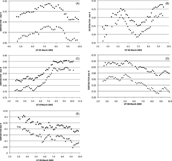
Figure 1. B and I microvariability observations of S5 0716+714 obtained on 2003 March 5 (A), March 6 (B), March 7 (C), March 8 (D), and March 9 (E). B-band observations are denoted by filled diamonds, I observations are denoted by filled circles.
Download figure:
Standard image High-resolution imageBelow we discuss the variability amplitudes and timescales observed on individual nights.
2003 March 5. On this night, we observed a 0.072 mag increase in brightness in B and 0.063 in I over the first 2.65 hr of observing, followed by a decline in brightness of 0.069 mag in B and 0.077 in I over 1.90 hr. There is evidence of smaller amplitude events superposed on this overall variation. The two most convincing of these is the event centered on UT 7.756, which has a depth of 0.02 mag in B and 0.02 in I and a duration of 0.66 hr. The second event is centered on UT 9.53, with duration of 0.39 hr and an amplitude of 0.011 in B and 0.011 in I.
2003 March 6. The variability this night was characterized by rapid increases and decreases in brightness. The source displayed a rise of 0.154 mag in B and 0.122 in I over 1.8 hr, followed by a decline in brightness of 0.130 mag in B and 0.103 in I over 1.54 hr, followed by a brightness increase of 0.139 in B and 0.126 in I over 2.42 hr.
2003 March 7. This night's observations began with a well-defined outburst with an amplitude of 0.043 mag in B and 0.045 mag in I, lasting for 1.67 hr and centered on UT 4.45. The source next brightened by 0.187 mag in B and 0.161 mag in I over 2.55 hr. At the end of the observation, there appears to be a well-defined outburst in the B band, with an amplitude of 0.018 mag lasting for 0.79 hr, though there is no obvious counterpart in the I band.
2004 March 8. This night begins with an event centered on UT 3.38 which lasted for 1.5 hr, with an amplitude of 0.031 mag in I and 0.020 mag in B, which is marginally significant given the error bars on B. The source next increased in brightness by 0.050 mag in I and 0.037 mag in B over 0.69 hr, followed by a steady decline in brightness of 0.160 mag in I and 0.124 mag in B over 3.43 hr. Superposed on this decline is evidence of small amplitude events of amplitude 0.01–0.02 mag which are clearly seen in both filters. The night's observation ends with another well-defined event with an amplitude of 0.050 mag in I and 0.036 mag in B and a duration of 1.18 hr.
2004 March 9. The night begins with a decline of 0.08 mag in B and 0.053 mag in I over the first 3.0 hr. Toward the end of this overall decline, there is a rapid decline of 0.065 mag in both filters, followed by an outburst centered on UT 6.5 with an amplitude of 0.05 mag in both filters. The source then rapidly brightens by 0.04 mag in both filters, remains at a constant level for 0.5 hr, then begins a gradual decline for about 1 hr. At the very end of this decline, another sharp drop in brightness occurs with an amplitude of 0.07 mag in both filters, followed by a recovery lasting to the end of the observations.
3.2. Color Analysis
2003 March 5. A plot of the flux in the I band versus the flux in the B band (FI versus FB) and a plot of the ratio of the flux in the B band to the flux in the I band versus the flux in the B band (FB/I versus FB) are shown in Figures 2(A) and (B). The flux units in B and I are arbitrary. The plot of FI versus FB shows a linear relationship between FI and FB with a Spearman correlation coefficient of 0.93 and a confidence factor of 1.4 × 10⁻¹⁷. The FB/I versus FB plot shows a counterclockwise hysteresis loop. We have connected the points in time to show this more clearly. As the source increases in brightness in the B band, it appears to stay within a confined range of FB/I. As it reaches and passes the peak of the variation, FB/I increases, then as the source fades, FB/I again remains confined in a narrow range, although higher than on the rising branch. A smaller loop is evident on the right-hand edge of the plot, this loop is in a clockwise direction and corresponds to the dip in the light curve centered on UT 7.75.
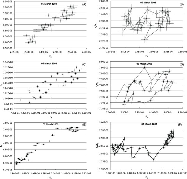
Figure 2. FI vs. FB and FB/I vs. FB observations of S5 0716+714 obtained on 2003 March 5–7. Panels (A)–(F) are the individual nights in time order, with FI vs. FB on the left side and FB/I vs. FB on the right side.
Download figure:
Standard image High-resolution imageWe define the significance of these loops in terms of a measure of their width in relation to the error bars. Since the loops are not circular, we choose and average of the long and short axis of these loops scaled to 1 error bar (σ). For this night, we find the loops range in significance from 2.5σ for the smallest loops to 4.9σ for the largest loop.
2003 March 6. The FI versus FB and FB/I versus FB plots are shown in Figures 2(C) and (D) for this night. The FI versus FB plot is linear, with a Spearman correlation coefficient of 0.96 and a confidence factor of 4.2 × 10⁻²⁴. The FB/I versus FB plot clearly shows a clockwise hysteresis loop with a significance of 16σ. This clockwise loop describes the dip in the light curve that runs from UT 5.8 to UT 9.3 in Figure 1(B). As the source brightens, FB/I remains relatively constant, as the peak is passed, FB/I decreases and remains relatively constant during the declining branch. Then as the source reaches a minimum and begins to increase in brightness again, FB/I returns to a relatively constant level, nearly identical to the iB/I values seen at the beginning of the observation.
2003 March 7. Figures 2(E) and (F) display the iI versus FB and FB/I versus FB plots. The FI versus FB plot shows a linear trend followed by a plateau, which is different from the strictly linear behavior the FI versus FB plots displayed the first two nights the source was observed. The plateau is coincident with the last two hours of variability seen in Figure 1(C). The Spearman correlation coefficient is 0.91 with a confidence factor of 8.49 ×10⁻²² for the linear portion of this plot. Counterclockwise loops are visible at the beginning and end of the FB/I versus iB plots, correlating with the mini-bursts seen at the beginning and end of this nights observation. These loops have a significance of 6.5σ for the loop corresponding to the beginning of the observation and 9.0σ for the loop corresponding to the end of the observation. In addition, a linear trend is visible corresponding to the last two hours of the observation, with FB/I increasing (becoming bluer) as FB increases.
2003 March 8. The FI versus FB curve (Figure 3(A)) shows a linear relationship over the entire observation, with a Spearman correlation coefficient of 0.96 ×10⁻³⁰. FB/I versus FB (Figure 3(B)) shows counterclockwise loops corresponding to mini-bursts and clockwise loops corresponding to dips in brightness. These loops range in significance from 4.5σ to 16σ.
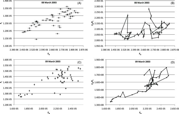
Figure 3. FI vs. FB and FB/I vs. FB observations of S5 0716+714 obtained on 2003 March 8 and 9. Panels (A)–(D) are the individual nights in time order, with FI vs. FB on the left side and FB/I vs. FB on the right side.
Download figure:
Standard image High-resolution image2003 March 9. Figures 3(C) and (D) show the FI versus FB and FB/I versus FB plots for this night. The FI versus FB plot is linear, with a Spearman correlation coefficient of 0.94 and a significance factor of 3.1 × 10⁻²². FB/I versus FB initially shows a slight increase in FB/I as FB increases, then exhibits the looping behavior seen in previous nights corresponding to the bursts and dips seen toward the end of this night's observations. The significance of these loops ranges from 24σ to 4σ.
3.3. Cross-correlation Results
The Z-transformed discrete cross-correlation (ZDCF) program of Alexander (1997) was applied to the observations to search for the presence of any lags. Magnitudes were converted to arbitrary flux and we searched for any lags between the flux in different wavelength bands and between FB and FB/I. The resulting plots of correlation coefficient R versus lag are shown in Figures 4(A)–(F) and Figures 5(A)–(D). Table 1 summarizes the results of this analysis. The lag was determined by fitting a Gaussian to the peak in the plot and the quoted errors are the errors on the Gaussian fit. In order for us to consider a lag meaningful, we require that the magnitude of the lag be greater than three times the data spacing, i.e., only lags greater than 0.39 hr (23 minutes) are considered meaningful. Using this criteria, no meaningful lags were found between the B- and I-flux variations for any of the five nights of observations. Three meaningful lags were found between FB/I and FB were on the nights of 2003 March 5, 2003 March 6, and 2003 March 7. A lag of 85.8 ± 1.8 minutes with R = 0.61 is seen on the night of 2003 March 5, where FB/I leads FB. On UT 2007 March 6, we find FB leads FB/I by 31.8 ± 0.02 minutes, with R = 0.44. A lag of 85.8 ± 0.6 minutes with an R = 0.59 was found on UT 2003 March 7, where FB/I was leading FB.
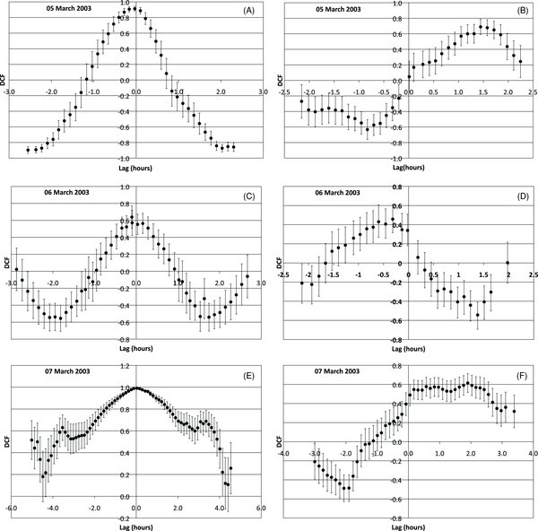
Figure 4. Z-transformed cross-correlations for March 5–7. Panels (A)–(F) are in time order, with the correlation curve for FB and FI on the left and FB and FB/I on the right.
Download figure:
Standard image High-resolution image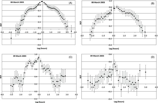
Figure 5. Z-transformed cross-correlations for March 8 and 9. Panels (A)–(D) are in time order, with the correlation curve for FB and FI on the left and FB and FB/I on the right.
Download figure:
Standard image High-resolution imageTable 1. Cross-correlation Results
| UT Date | Lag Between FB and FI (minutes) | Lag Between FB and FB/I (minutes) |
|---|---|---|
| 2003 Mar 5 | −9.51 ± 0.002 | 85.8 ± 1.8 |
| 2003 Mar 6 | 0.6 ± 0.6 | −31.8 ± 0.02 |
| 2003 Mar 7 | 5.7 ± 0.14 | 85.8 ± 0.6 |
| 2003 Mar 8 | −6.9 ± 1.2 | 20.9 ± 3.0 |
| 2003 Mar 9 | −10.20 ± 1.8 | 1.32 ± 4.8 |
Download table as: ASCIITypeset image
In order to obtain a determination of the significance of these lags, we set out to determine how often such lags might occur by chance. Using a Monte Carlo type methodology, pairs of B and I light curves were simulated using the slopes of the PDS found for a given nights B and I light curves. B/I flux ratios and light curves were determined and the data were sampled consistent with the sampling of the actual observations. The ZDCF algorithm was applied to these time series, and we determined the percentage that any lag with the same or better quality (as defined by the cross-correlation coefficient R) was detected. We also determined the percentage that a lag of the same sign would occur. For 2003 March 5, we find a lag of the same or better quality randomly occurs 10% of the time and a positive lag of the same or better quality occurred 6% of the time. The night of 2003 March 6, we find a lag of the same or better quality randomly occurs 18% of the time and a negative lag of the same quality occurs 10% of the time. On 2006 March 7, we find a lag of the same or better quality randomly occurs 10% of the time and a positive lag of the same or better quality occurs 2% of the time. This leads us to conclude the detected lags are significant.
3.4. Structure Functions
A structure function analysis was applied to the data from both filters on all five nights. From such an analysis one can derive the slope of the structure function, which is related to the type of process associated with the times series (red noise, white noise, flicker noise, etc.). We found that for the nights of March 5–7, the structure functions resembled each other, displaying a linear rise to a turnover at a lag related to a characteristic variability timescale (Figures 6(A)–(F)). The last two nights, March 8 and 9 (Figures 7(A)–(D)), the structure functions displayed far more complex structure with multiple breaks and plateaus, indicative of several different variability timescales present in the data. Slopes were determined via linear fits in the range between three times the data spacing and 2/3 the length of the data train except for the last two nights, where we measured the slopes on either side of any detected breaks or plateaus. On March 8, we see a slope of in B of 1.36 and 0.98 in I up to timescales of 1 hr. Between 1 and 1.6 hr, the SF is mostly flat, from timescales of 2 hr up to 2.4 hr, the SF has a slope of 1.5 in B and 1.02 in I. On March 9, we see a slope in B of 0.60 up to timescales of 0.8 hr. Between 0.8 and 0.93 hr, the structure function (SF) is mostly flat, from timescales of 0.93 hr up to 1.95 hr, the SF has a slope of 1.68 in B. The structure function plateaus a second time, from 1.95 hr to 2.29 hr, then steepens to a slope of 2.22 from 2.29 to 2.86 hr. After 2.86 hr, it abruptly flattens until 3.24 hr then rises with a slope of 1.03 to timescales of 4.2 hr. In I we see a slope of 0.60 up to timescales of 0.78 hr. From 0.78 to 1.05 hr there is an abrupt decrease and then flattening. From 1.05 hr up to 1.82 hr the structure function has a slope of 1.5. There seems to be a much larger degree of low amplitude, very rapid microvariability on this night, which is contributing to the disparity in the structure function results between the two wavebands. The results are summarized in Table 2.
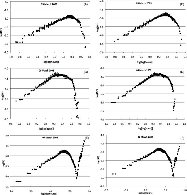
Figure 6. Structure functions for March 5–7, in time order with the structure function for the B-band observations on the left side of the page and the structure function for the I-band observations on the right side of the page.
Download figure:
Standard image High-resolution image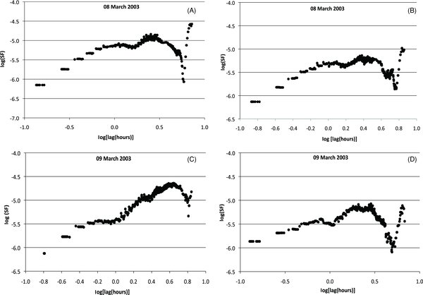
Figure 7. Structure functions for March 8 and 9, in time order with the structure function for the B-band observations on the left side of the page and the structure function for the I-band observations on the right side of the page.
Download figure:
Standard image High-resolution image
Table 2. Structure Function Slopes
| UT Date | Slope of the B-band SF | Slope of the I-band SF |
|---|---|---|
| 2003 Mar 5 | 1.24 | 1.48 |
| 2003 Mar 6 | 1.57 | 1.59 |
| 2003 Mar 7 | 1.21 | 1.22 |
| 2003 Mar 8 | 1.36, 1.5 | 0.98, 1.02 |
| 2003 Mar 9 | 0.6, 1.68, 2.22, 1.03 | 0.6, 1.5 |
Download table as: ASCIITypeset image
3.5. I-band Calibration of Star 4
The data set we have obtained allows us to determine a differential calibration of the I-band magnitude of comparison star 4 from the sequence of Villata et al. (1998), which is not included in the I-band calibration of the comparison stars in this field of Ghisellini et al. (1997). We determined the I-band magnitude of star 4 with respect to stars 6, 5, and 3 of Ghisellini et al. (1997) for each night, then averaged these values to obtain an magnitude with respect to each comparison star. We then averaged these values to obtain an I-band magnitude for star 4 of 12.645 ± 0.003.
4. DISCUSSION
4.1. Limits to the Size of the Emission Region
During the course of these observations, complete events with a variety of timescales were observed. Invoking light travel time arguments, we can use the timescales of such events to define upper limits to the size of the emission regions responsible for the variations. The maximum timescale event that was observed was the event on 2003 March 5, which has a timescale of 4.55 hr. The shortest observed events occurred with timescales of 30– 60 minutes and were seen throughout the data; we will take 30 minutes as the lower limit to the shortest timescale variation seen. Invoking light travel time arguments, i.e., R ⩽ δcΔt we find that the regions responsible for the observed microvariability range in size from R ⩽ 5.38 ×10¹³δ cm to R ⩽ 4.90 ×10¹⁴δ cm. Adopting the value of δ = 20 from Nesci et al. (2005), we find this range to be R ⩽ 1.07 ×1015 cm to R ⩽ 9.8 ×1015 cm.
4.2. Hysteresis Loops and Cross-correlations
Lags observed between FB and FB/I and hysteresis loops arise when the information about a variation propagates through the spectral energy distribution. In the model proposed by Kirk et al. (1998) hysteresis loops are expected, and their directionality is a function of the observed frequency and the frequency at which the synchrotron emission component peaks. In this model, one would expect to see only clockwise loops for bursts in S5 07176+1714, since these optical observations are at a frequency far below the peak synchrotron frequency in this source, where the cooling rate for the electrons is much slower than their acceleration rate. However, we see counterclockwise loops for bursts in the observations presented here, opposite what is expected in this model. Inspection of the light curves presented in Figures 1((A)–(E)) shows that the flares are all symmetric, with the exception of the night of 2003 March 5. However, one could easily argue that the observations did not cover the entire flare that night and that if they did one would see a symmetric shape to the flare. If the observed microvariability is the result of local turbulence in the jet and the light crossing time of these turbulent regions is longer than the cooling and particle injection timescales in these regions, symmetric flares (Xilouris et al. 2006) are expected. This leads us to conclude the observed variations are determined by the size of the turbulent regions and not the electron cooling or acceleration timescales intrinsic to those regions.
4.3. Structure Functions
Table 2 gives the slope(s) of the structure function for each filter on each night. The slopes mostly lie between 1.0 and 2.0 in a region which indicates a fractional noise process (Mandelbrot & Van Ness 1968). This is similar to the result found by Azarnia et al. (2005) who analyzed 10 separate microvariability time series via Fourier analysis. Such a process is expected from turbulent phenomena, thus these results are completely consistent with an interpretation that microvariability arises from turbulent phenomena. The location of the turbulence cannot be determined from these observations, but is most likely within the relativistic jet (Marscher et al. 1992) though there are models within which this turbulence would reside within the accretion disk (Mangalam & Wiita 1993; Chakrabarti & Wiita 1993). No obvious dependencies of the slope on wavelength band are present though we obtained different results between wavebands on the night of March 9th as discussed above. Table 3 gives the variability timescales derived from the turnover or breaks identified within each structure function. The derived timescales are consistent between the two passbands, with the greatest discrepancy again on the night of March 9.
Table 3. Structure Function Variability Timescales
| UT Date | B Timescales (hr) | I Timescales (hr) |
|---|---|---|
| 2003 Mar 5 | 2.17 | 2.21 |
| 2003 Mar 6 | 2.10 | 2.10 |
| 2003 Mar 7 | 2.20 | 2.21 |
| 2003 Mar 8 | 2.64 | 2.69 |
| 2003 Mar 9 | 4.25 | 2.53 |
Download table as: ASCIITypeset image
5. CONCLUSIONS
Five consecutive nights of continuous observations of S5 0716+714 in the B and I bands display variability on timescales from tens of minutes to days. The timescale of discrete events observed in the light curve constrain the size of the emission regions responsible for these events from R ⩽ 1.07 ×1015 cm to R ⩽ 9.8 ×1015 cm. The B- and I-band variations are highly correlated, with no detectable lags between bands. Significant lags were detected between the flux in the B band(FB) and the B/I flux ratio (FB/I) on three nights. Hysteresis loops are present in the B versus B/I plots, these loops are clockwise for dips in the light curve and are associated with detected lags between FB/I and FB in the sense that FB/I lags FB. The loops are counterclockwise for bursts and are associated with detected lags between FB/I and FB in the sense that FB/I leads FB. The directionality of the hysteresis loops and the symmetric nature of the flares are consistent with the flux variations being dominated by the light crossing time of the emission region and not its intrinsic electron cooling or acceleration timescales. A structure function analysis indicates that the variations can be characterized as a fractional noise process, consistent with the interpretation that the variations arise as a result of turbulent process, quite likely located in the relativistic jet. The large body of data allows us to provide a differential calibration of the I-band magnitude for comparison star 4 from Villata et al. (1998) of I = 12.645 ± 0.003.
We thank Lowell Observatory for generous allocations of observing time for our investigations of the microvariability phenomena in AGNs. M.T. Carini wishes to thank Western Kentucky University, the Applied Research and Technology Program at WKU, and the Kentucky Space Grant Consortium for supporting various aspects of this work. The authors also thank the referee for very helpful comments and suggestions.
Footnotes
- 2
IRAF is distributed by the National Optical Astronomy Observatory, which is operated by the Association of Universities for Research in Astronomy, Inc. under contract to the National Science Foundation.