


ABSTRACT
The Voyager flybys of Saturn in 1980–1981 revealed a circumpolar Hexagon at ∼78° north planetographic latitude that has persisted for over 30 Earth years, more than one Saturn year, and has been observed by ground-based telescopes, Hubble Space Telescope and multiple instruments on board the Cassini orbiter. Its average phase speed is very slow with respect to the System III rotation rate, defined by the primary periodicity in the Saturn Kilometric Radiation during the Voyager era. Cloud tracking wind measurements reveal the presence of a prograde jet-stream whose path traces the Hexagon's shape. Previous numerical models have produced large-amplitude, n = 6, wavy structures with westward intrinsic phase propagation (relative to the jet). However, the observed net phase speed has proven to be more difficult to achieve. Here we present numerical simulations showing that instabilities in shallow jets can equilibrate as meanders closely resembling the observed morphology and phase speed of Saturn's northern Hexagon. We also find that the winds at the bottom of the model are as important as the winds at the cloud level in matching the observed Hexagon's characteristics.
Export citation and abstract BibTeX RIS
1. INTRODUCTION
Saturn's northern Hexagon is a planetary-scale cloud band that has six well-defined corners and encircles the north pole of Saturn at5
 N (Figure 1). It was discovered by Godfrey (1988) in Voyager images captured in 1980–81, and it has persisted for more than one Saturn year (
 Earth years) (Caldwell et al. 1993; Sánchez-Lavega et al. 2014). Observations by Voyager and Cassini have revealed the following key characteristics of the Hexagon: (1) it is associated with an eastward zonal jet at 78° N which has a peak speed of
  , as determined from tracking individual cloud patterns forming the Hexagon (Godfrey 1988; Baines et al. 2009; Sánchez-Lavega et al. 2014); (2) the path of the zonal jet follows the outline of the hexagonal cloud morphology; (3) there is no evidence that the Hexagon is a "vortex-street," a series of spots of alternating vorticity staggered on the flanks of the jet; (4) measurements from Voyager images yielded a speed for the vertices of the Hexagon of
  (Godfrey 1988). Measurements based on more recent Cassini observations yield a speed of
  (Sánchez-Lavega et al. 2014). Therefore, the Hexagon's net phase speed is very small relative to the Voyager-era radio period of the Saturn Kilometric Radiation of 10h 39m 24s (Desch & Kaiser 1981), which forms the basis for the currently defined System III rotation period for Saturn (Seidelmann et al. 2007), and corresponds to a planetary angular velocity
  . All quantities presented in this paper are measured in this reference frame; and (5) there is a meridional temperature gradient associated with the Hexagon in the 100–800 mbar region, with the equatorial side of the jet being colder than the polar side (Fletcher et al. 2008). Here we present results of numerical simulations that reproduce all five observed characteristics of Saturn's northern Hexagon.
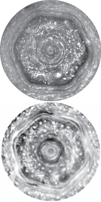
Figure 1. Hexagon observations from Cassini-ISS (Sayanagi et al. 2009; top), and Cassini-VIMS (Baines et al. 2009; bottom).
Download figure:
Standard image High-resolution image2. MODEL SETUP
Our simulations tested the evolution of Gaussian eastward jets of the form

to perturbations of their associated Montgomery stream function described by
where λ is the planetographic latitude,  is the meridional distance from the center of the jet, U0 is the peak velocity or amplitude of the jet, b is the peak latitudinal curvature of the jet, δ is the amplitude of the perturbation,
  is the planetographic latitude of the center of the jet, a0 is the FWHM of the perturbation, P is the pressure, P0 is the pressure level where the perturbation is added, c0 is the vertical extension of the perturbation in scale heights, k is the east-west planetary wavenumber, ϕ is the longitude,
  is a random phase offset, and L is the total number of wavenumbers included in the perturbation, which we set to be 50.
The model used in this study is the Explicit Planetary Isentropic-Coordinate General Circulation Model developed by Dowling et al. (1998). This model integrates the hydrostatic primitive equations on an oblate sphere. The nominal domain consists of a channel that spans 360° in the longitudinal direction and that extends from 67 3 to 873 in the latitudinal direction, with a resolution of
  km at the jet location, which is adequate to resolve the estimated deformation radius at this latitude (
 km; Read et al. 2009). In the vertical direction, the model has 20 layers equally spaced in
  that extend from 0.1 mb to 10 bars, with the five top layers set as a damper of vertically propagating waves (i.e., "sponge" layers). The model uses a high-latitude low-pass filter that leaves low planetary wavenumbers (
 ) unaffected in the location of the jet center. This filter ensures numerical stability in the northernmost boundary where the grid spacing is smaller. A high-order viscosity term is used to dampen computational modes, and a Rayleigh forcing term is used to compensate for the loss of zonal kinetic energy from our eastward jet through shear instabilities.
Our simulations adopt a vertical thermal profile as a function of pressure above 1 bar that resembles the observed temperatures measured by Cassini CIRS during Saturn's northern winter in 2007 (Fletcher et al. 2008). Below that level this profile is extrapolated to approach different constant target values of the Brunt–Väisälä frequency at the bottom of the model. The nominal value for N at the bottom of the model is set to be  .
.
With this set-up, the space of parameters explored by our simulations consists of variations in the jet amplitude (U0), the jet curvature (b), the vertical shear of our Gaussian wind profile above 2 bars, the vertical wind shear below the same level, the zonal winds at the bottom of the model, and the static stability of the atmosphere below 1 bar. The model's response to perturbations like the one described by Equation (2) is then compared to observations of the Hexagon. The criteria applied to validate our model output against the observations and to guide our free parameter exploration consisted of checking for the following characteristics in the model output: (1) the jet evolves and equilibrates into a meandering state and not into a vortex-street, so that at the end of the simulation, the jet is not flanked by alternating patches of cyclonic and anticyclonic vorticity; (2) the final wind profile describing the jet is within the error bar of the observed wind profile; (3) the drift rate of the meander that forms is close to the observed propagation of the Hexagon; and (4) there is a temperature gradient associated with the Hexagon, the equatorial side of the jet being colder than the polar side.
3. SIMULATIONS
In this section, we present three series of simulations with distinct outcomes. The first series of simulations we present are analogous to those presented by Morales-Juberías et al. (2011), in which the wind structure is assumed to be deeper than the simulation domain. For this structure of zonal winds the model always equilibrates into a vortex-street, independently of the value of the other parameters. The left column of Figure 2 shows the results of initializing the model with a Gaussian jet characterized by an amplitude of  and curvature of
  that remains constant with altitude below 2 bars. When the model is seeded with a perturbation, Equation (2), it equilibrates very rapidly (after 25 days
 ![$[1\;{\rm day}=24\;{\rm hr}]$](https://content.cld.iop.org/journals/2041-8205/806/1/L18/revision1/apjl514943ieqn17.gif) ) into six pairs of interlocking cyclones and anticyclones that form a vortex-street. The time evolution of the relative vorticity at the peak of the jet shows that, after its rapid emergence, the vortex-street propagates to the east at
) into six pairs of interlocking cyclones and anticyclones that form a vortex-street. The time evolution of the relative vorticity at the peak of the jet shows that, after its rapid emergence, the vortex-street propagates to the east at  , which is significantly faster than the observed Hexagon propagation speed. While variations in the other parameters explored in this case (U0, b, and N) change the dominant wavenumber in the vortex-street and its propagation rate (as in Morales-Juberías et al. 2011), the result is always a vortex-street that propagates too fast to the east. In all of these simulations, the growth of the instability widens and weakens the jet, reducing its peak speed (Figure 3).
Figure 2. Comparative results of the three series of simulations described in the text. The left column shows the results for a simulation initialized with a Gaussian jet that remains constant with altitude below 2 bars. The middle column shows the results for a simulation initialized with a Gaussian jet that decreases to zero at the bottom of the model below 2 bars. The right column shows the results of a simulation initialized with Gaussian jet that decreases to the bottom level winds as shown in Figure 3. In all cases the polar plots in the middle show the potential vorticity after 500 simulated days, and the bottom plots show the time evolution of the relative vorticity at the center of the jet. The values of U0 and b in each case are those that evolve into a dominant wavenumber of six for the different vertical wind configurations, so that a morphological comparison is possible with the same wavenumber.
Download figure:
Video Standard image High-resolution image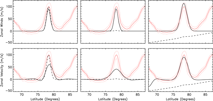
Figure 3. Zonal wind profiles at  bar (thick black line) and at the bottom of the model (thick dashed line) at day 0 (top row) and day 500 (bottom row) for the simulation results shown in Figure 2. The red solid line is the observed zonal wind, and the red dashed line marks the confidence lines of the observed winds (Antuñano et al. 2015).
Download figure:
Standard image High-resolution imageIn the second series of simulations, we assume that the wind structure is shallower than the model domain. This initial wind profile equilibrates in a hexagonal, meandering jet. The middle column of Figure 2 shows the results of initializing the model with a Gaussian jet characterized by an amplitude of  and curvature of
  that decreases to zero at the bottom of the model below 2 bars. When we seed the model with a perturbation, Equation (2), its path equilibrates into a stable meander with a dominant zonal wavenumber of six as shown in the polar projected maps of potential vorticity after 500 days. The time evolution of the relative vorticity at the center of the jet shows that after forming, the meander propagates slowly to the east with a speed of
  This speed is slower than the vortex-street case, but it is still faster than that of the observed Hexagon. While variations in the other parameters (U0, b, and N) explored in this configuration can alter the dominant wavenumber and propagation rate of the meanders formed, all the meanders produced this way fail to meet one or more of our criteria described above. In other words, either the wavenumber at the end of the simulation is not six, the propagation speed is faster to the east than the observed propagation rate, or the final shape of the jet is beyond the error of the observed jet. In this group of simulations, the growth of the instability also widens and weakens the jet, reducing its peak speed (Figure 3).
In the third series of simulations, we keep the cloud-top 1 bar wind speed observed in the inertial frame identical to those in the first two series, but we make it decrease toward a wind profile at the bottom of the model as shown in top-right panel of Figure 3. The right column of Figure 2 shows the results of initializing the model in this way for a Gaussian jet characterized by an amplitude of  and curvature of
  . For vertical structure of the jet, after 400 simulated days, the model equilibrates into a stable meander with a dominant wavenumber of six. This meander is practically stationary, and its amplitude is smaller than those in our second series of simulations. Thus when projected into a polar map, it has a sharp hexagonal shape instead of a star-like shape (see Figure 8 in Antuñano et al. 2015). Furthermore, the meander produced this way matches all the observed dynamical properties of Saturn's northern Hexagon. There are no vorticity patches associated with the meandering of the jet (i.e., not a vortex-street), the zonal winds at the end of the simulation are within the observed errors of the measured winds in the location of the jet where the Hexagon exists, and the propagation rate of the meander (
 ) is practically stationary.
4. DISCUSSION
Past numerical and laboratory modeling efforts have succeeded in reproducing some, but not all, of the Hexagon's characteristics. Allison et al. (1990) interpreted this feature to be a stationary Rossby wave perturbed by the anticyclonic vortex observed to the south of the eastward jet and meridionally trapped by the relative vorticity gradient of the flow itself. Barbosa-Aguiar et al. (2010) showed how polygonal patterns, corresponding to wave modes excited by the nonlinear equilibration of a barotropically unstable zonal jet, can appear in laboratory experiments of flows in a rotating tank. Those patterns are associated with a vortex-street, and their sharpness and rotation can be adjusted with the slope at the bottom of the tank (which simulates a weak topographic β-effect). Morales-Juberías et al. (2011) presented numerical simulations like the first series of simulations described here in that the wind structure was assumed to be deeper than the simulation domain, and the hexagonal structure that emerged was a vortex-street with a net phase speed too high compared to the observed value.
At the latitude of the Hexagon, the beta parameter ( , where
  is the Coriolis parameter) is very small compared to the second derivative of the mean zonal wind, and the necessary, but insufficient, Rayleigh-Kuo criterion for barotropic stability is easily violated (Ingersoll et al. 1984; Read et al. 2009). The Gaussian jets adopted in our simulations violate the Rayleigh-Kuo criterion, and past linear stability analyses demonstrate that barotropic instabilities indeed arise in such profiles (Holland & Haidvogel 1980). Flierl et al. (1987) studied the nonlinear evolution of barotropic beta plane jets as a function of the beta parameter and the dominant wavenumber of a perturbation to the stream-function. Within this space of parameters, they showed how jets can equilibrate forming either a stable vortex-street or a steady meander. Our Gaussian jets also have reversals in their zonal mean potential vorticity profiles, which represent a violation of the Charney–Stern stability criterion (Charney & Stern 1962). Previous studies have also shown how baroclinic instabilities can equilibrate into meanders in such profiles (Koschmieder & White 1981; Bastin & Read 1997; Sutyrin et al. 2001). Other experiments have shown how polygonal patterns can emerge in flows for a wide range of parameters and different kinds of forcing (Sommeria et al. 1989; Vatistas 1990; Vatistas et al. 1994; Marcus & Lee 1998; Jansson et al. 2006).
Here, we have shown that small perturbations to the stream-function of an eastward Gaussian jet can grow and equilibrate as a vortex-street or as a meander, depending on the vertical wind shear and the wind profile at the bottom of our model. Our Gaussian jets violate the criteria for barotropic and baroclinic instability, but violations of these criteria do not determine which instability type will be dominant in the simulations. In general, barotropic instabilities in quasi-geostrophic jets are due to strong horizontal gradients of vorticity and are associated with transfer of kinetic energy from the mean flow to the perturbation. Baroclinic instabilities are due to the tilting of the isobaric surfaces, and are associated with transfer of potential energy from the zonal flow to the perturbation. In our first two series of simulations the jet decreases in amplitude and widens significantly as the simulations evolve (Figure 3), which is a characteristic signature of barotropic instability (Pedlosky 1982). In our third series of simulations, the jet amplitude and shape are left relatively unaltered throughout the simulation (Figure 3), and thus we speculate that barotropic instability is not the dominant instability in this case.
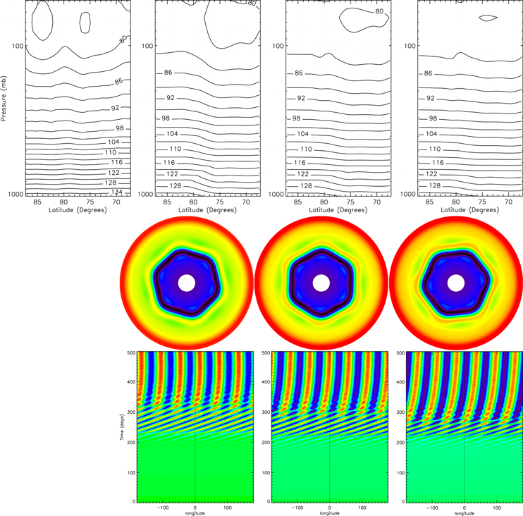
Figure 4 shows the comparison between the temperatures observed in Saturn retrieved from CIRS observations with Cassini (Fletcher et al. 2008) and the model's temperatures after 500 simulated days for three cases in our third series of simulations that differ only in the vertical shear of the Gaussian wind profile above 2 bars. Between 76° N and 80° N, our model shows in all cases a temperature gradient that corresponds to the decay of the hexagonal jet with altitude. Changing the vertical wind gradient in the top of the model can flatten the model's meridional temperature gradient in that pressure range without significantly affecting the dynamical properties of the resulting meander (i.e., dominant wavenumber stays at six and the propagation speed remains slow), since those are fundamentally controlled by the vertical shear and the shape of the winds at the bottom of the model. This model behavior reproduces the seasonal insensitivity of the Hexagon's characteristics to seasonal changes observed in the 70–250 mb region (Fletcher et al. 2010, 2015). Sánchez-Lavega et al. (2014) attributed this insensitivity to the seasonal effects observed by CIRS as evidence that the Hexagon must be a deep-rooted feature. Our results show that a jet shallower than the model domain can produce a hexagon that matches all the observed properties of Saturn's Hexagon and is also insensitive to "seasonal" changes at the top of the model. Outside of the 76° N and 80° N region, our background wind field lacks the additional eastward and westward jets at other latitudes to be able to reproduce the temperature gradients associated with those jets. At altitudes above the 500 mbar pressure level, our temperatures are on average 3 K higher than the observed temperatures which have an error of  K. This 3 K deviation could be due to physical processes that are not included in our modeling such as heating and cooling by absorbers in those levels of the atmosphere.
Figure 4. Top left: mean zonal temperatures observed in Saturn (Fletcher et al. 2008). Top: mean zonal temperatures at 500 days for three cases in our third series of simulations that differ only in the vertical shear of the Gaussian wind profile above 2 bars. From left to right: the wind profile decays to zero in 10, 14, and 18 scale heights, respectively. Middle: polar projections of the potential vorticity after 500 simulated days. Bottom: time evolution of the relative vorticity at the center of the jet for the three different cases. The propagation speed of the meander in the last 100 days is  , 0.1, and
  , respectively.
Download figure:
Standard image High-resolution image
Finally, to test the effect of the latitude on the evolution of the perturbations, and to address the question of why we do not observe a Hexagon in the Southern Hemisphere jet located at  S, we ran a preliminary series of simulations implemented with a Gaussian jet like the one used in our third series of simulations placed at different latitudes from 75° to 30° (in 5° intervals). We do not observe instabilities growing when the center of the jet is placed between 75° and 40°. For the cases when the jet center is placed at 35° and 30°, the jet equilibrates in a state that is more reminiscent of the morphology of the Ribbon (Godfrey & Moore 1986; Sayanagi et al. 2010) than that of the Hexagon. In a future study we will explore this latitude variation with more detail including more parameters, like the width and amplitude of the jet and the structure of the jet at the bottom of the model. Cassini proximal orbits will likely be able to better constrain the depth and structure of the zonal flows in Saturn at all latitudes, although being mostly near the equator, there will be higher uncertainty toward high latitudes of the planet like the one where the Hexagon is present.
5. CONCLUSIONS
We have shown that small perturbations to the stream-function of an eastward Gaussian jet can grow and equilibrate either as a vortex-street pattern or as a meandering jet depending on the vertical shear of the jet: deep jets evolve into vortex-streets and shallow jets evolve into meanders. In our simulations, the initial amplitude (U0) and curvature of the jet (b) determine the dominant wavenumber, similar to results in Morales-Juberías et al. (2011). We also find that the winds at the bottom of the model are as important as the winds at the cloud level in matching the observed Hexagon's characteristics, in particular its drift rate and its shape sharpness. In addition, we show that the model behavior reproduces the insensitivity of the Hexagon's characteristics to seasonal changes observed in the 70–250 mb region, since the morphology and propagation rate of the hexagon in our model is fundamentally controlled by the vertical shear and the shape of the winds at the bottom of the model.
This work was partially supported by NASA PATM grant number NNX14AH47G to A.S., and NASA OPR grant NNX12AR38G and NSF A&A grant 1212216 to K.M.S. L.N.F. was supported by a Royal Society Research Fellowship at the University of Oxford. Computational resources were provided by New Mexico Tech. -
Footnotes
- 5
Latitudes are planetographic unless otherwise noted.