

Abstract
We report on a combined experimental and modelling approach towards the design and fabrication of efficient bulk shields for low-frequency magnetic fields. To this aim, MgB2 is a promising material when its growing technique allows the fabrication of suitably shaped products and a realistic numerical modelling can be exploited to guide the shield design. Here, we report the shielding properties of an MgB2 tube grown by a novel technique that produces fully machinable bulks, which can match specific shape requirements. Despite a height/radius aspect ratio of only 1.75, shielding factors higher than 175 and 55 were measured at temperature T = 20 K and in axially-applied magnetic fields μ0Happl = 0.1 and 1.0 T, respectively, by means of cryogenic Hall probes placed on the tube's axis. The magnetic behaviour of the superconductor was then modelled as follows: first we used a two-step procedure to reconstruct the macroscopic critical current density dependence on magnetic field, Jc(B), at different temperatures from the local magnetic induction cycles measured by the Hall probes. Next, using these Jc(B) characteristics, by means of finite-element calculations we reproduced the experimental cycles remarkably well at all the investigated temperatures and positions along the tube's axis. Finally, this validated model was exploited to study the influence both of the tube's wall thickness and of a cap addition on the shield performance. In the latter case, assuming the working temperature of 25 K, shielding factors of 105 and 104 are predicted in axial applied fields μ0Happl = 0.1 and 1.0 T, respectively.
Export citation and abstract BibTeX RIS
1. Introduction
The ability to shield an external magnetic field or to act as a permanent magnet are two superconducting bulk applications that have attracted remarkable interest in the last few years. Different shaped vessels made out of superconducting compounds such as cuprate superconductors [1, 2] and MgB2 [3, 4] have been proved to mitigate magnetic fields larger than 1 Tesla. Besides, it has been shown that magnetic fields exceeding 3 T can be trapped by REBa2Cu3O7−x (RE = rare earth) [5, 6] and MgB2 [7–10] disks or disk-stacks.
Although MgB2 requires lower operating temperatures than cuprate superconductors, this compound presents characteristics attractive for bulk applications such as lower cost of the starting elements coupled with the absence of rare-earths, lighter weight and longer coherence lengths than cuprate superconductors. This last feature enables the flow of high critical current density, Jc, also in polycrystalline samples with randomly oriented grains, even when joints are present [11, 12]. As a result, large-size MgB2 bulk samples with almost isotropic properties and homogeneous Jc can be fabricated [9]. In addition, some processing techniques [13–16] have evidenced the possibility of manufacturing near net shape MgB2 bulks meeting specific application requirements [17].
The ability to shape and size the superconducting material is a key aspect for magnetic shielding applications in order to reach high performances of magnetic mitigation in relation to working conditions (field source, size of the area to be shielded, space constraints, just to name a few). Another key aspect is the availability of modelling techniques that can guide the devices' design, avoiding over-manufacturing and reducing experiment time/costs. In the last few years several numerical techniques have been proposed for modelling superconductors [18, 19]. However, their successful application requires accurate inputs, such as in-field Jc behaviour. Usually, Jc values are obtained by measurements on small samples cut from a larger bulk, but this procedure can lead to overestimations, even in homogeneous samples [20].
In this paper, we investigate the shielding properties of an MgB2 tube produced via an innovative technique that produces fully machinable MgB2 bulks [21], which can be shaped as required by specific applications. As in our previous studies [15, 22], we deal with a system with an aspect ratio of height/outer radius close to unity, in order to explore magnetic mitigation solutions in situations, such as space applications [23, 24], requiring minimum shield size/mass. Starting from the local magnetic induction field cycles measured along the tube's axis by means of cryogenic Hall probes, we calculated the macroscopic Jc flowing in the tube. To achieve this aim, we propose a two-step procedure that, considering the methodology described by Bartolomé et al [25], allowed us to reconstruct the current density dependence on magnetic field, Jc(B). The comparison of the experimental magnetic induction curves with those computed by numerical simulations where the superconductor is modeled by the so-achieved Jc(B), supports our approach and opens to investigations of more efficient shielding designs by numerical simulations.
The paper is organized as follows. In section 2, experimental details concerning the MgB2 growing technique and the characterization procedure are given. Section 3 deals with the experimental results of the shielding experiments. In section 4 we present the starting analytical method used for a preliminary Jc calculation and the numerical model exploited to compute the magnetic induction field. The critical current density dependence on magnetic field is discussed in section 5, where the comparison between the experimental and computed magnetic induction cycles is also reported. Finally, section 6 focuses on the effects of the tube's wall thickness and of cap addition on the shield performance and in section 7 the main outcomes are summarized.
2. Experimental details
2.1. MgB2 fabrication process
Commercial MgB2 powders (Alfa Aesar) were mixed with hexagonal BN. The powders were loaded into a graphite die system of ∼20 mm inner diameter and processed by spark plasma sintering (FCT System GmbH—HP D 5, Germany) at 1150 °C [26]. The as-obtained cylinder had an average relative density of 91%, height of 18.7 mm and radius of 10.15 mm. Hexagonal BN is inert with respect to MgB2 and allows the shaping of the sintered composite by machining [21]. The cylinder was drilled by using bits with different radii up to 7 mm. The inner radius of the final product was obtained by means of a lathe machine. The final height of the tube is h = 17.5 mm. Its inner and external radius are Ri = 7.0 and Ro = 10.15 mm, respectively (figure 1).
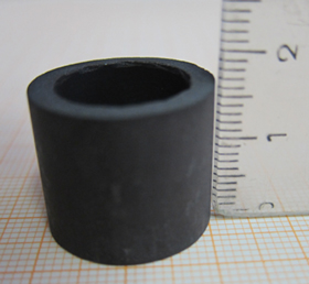
Figure 1. MgB2 cylinder obtained by spark plasma sintering, drilling and splintering on a lathe machine.
Download figure:
Standard image High-resolution imageThe irreversible temperature, assumed as the temperature where any magnetic signature of trapped field disappears, is Tirr = 37.4 K.
2.2. Measurement details
The MgB2 tube was mounted in tight thermal contact with the second cold stage of a cryogen-free cryocooler positioned in the bore of a superconducting cryogen-free solenoid. The sample was placed with its axis either parallel (axial field configuration) or perpendicular (transverse field configuration) to the coil axis. The magnetic induction field was measured by four cryogenic Ga–As Hall probes [27] located along the tube's axis in the positions reported in figure 2. The probes were always oriented to measure the component of the magnetic induction parallel to the applied magnetic field, for both the axial and transverse configurations.
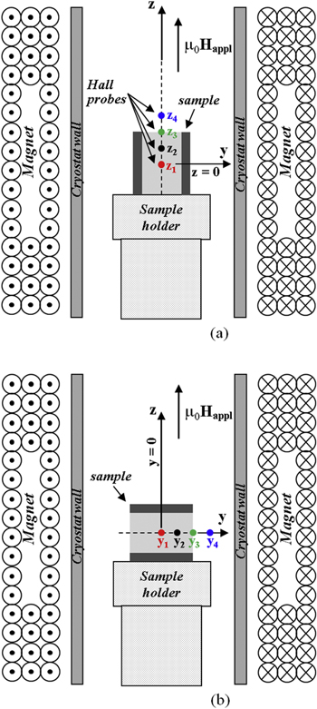
Figure 2. Schematic drawing of the experimental setup (not to scale) for the axial (a) and transverse (b) magnetic field configurations. Assuming z = 0 the position of the tube's centre in the axial field configuration, the Hall probes were located at z1 = 0, z2 = 4.4 mm, z3 = 8.8 mm (namely, in correspondence of the sample edge coordinate) and z4 = 13.1 mm. Similarly, assuming y = 0 the position of the tube's centre in the transverse field configuration, the Hall probes were located at y1 = 0, y2 = 4.4 mm, y3 = 8.8 mm (corresponding to the sample edge coordinate) and y4 = 12.0 mm. The Hall probes were always oriented in order to measure the component of the magnetic induction parallel to the applied field.
Download figure:
Standard image High-resolution imageAfter cooling in zero field condition, the applied field was cycled keeping fixed the sample temperature while the magnetic induction was recorded. The sample temperature, the applied magnetic field and the Hall probe voltages were controlled and/or driven by means of a LabVIEW software.
3. Magnetic shielding properties
We investigated the magnetic behaviour of the sample in the temperature range from 20 to 35 K. The main frame of figure 3 shows the magnetic induction, Bz, measured at T = 25 K along the tube's axis as a function of the cycled applied field, μ0Happl, in axial field configuration. The corresponding shielding factors (SFs), calculated as the ratio μ0Happl/Bz, i.e. the ratio of the applied field over the magnetic induction measured along the first-magnetization curve of the cycle, are reported in the inset.

Figure 3. Magnetic induction measured at T = 25 K by the four Hall probes positioned along the tube's axis as the applied field was cycling (main frame). The measurement was performed in the axial field configuration. In the inset the SFs—calculated as μ0Happl/Bz from the virgin branches of the hysteresis loops—are plotted.
Download figure:
Standard image High-resolution imageDespite the height/outer radius aspect ratio of only 1.75, which makes the magnetic flux penetration from the tube edge not negligible, at T = 25 K the shielding factor exceeds 160 and 34 at z1 and z2 positions, respectively, when the external field μ0Happl = 0.1 T is applied. This makes the shield competitive with systems with similar aspect ratio [2], as confirmed also by the shielding performance characterization at other temperatures. Figure 4 shows the SFs measured in the tube's centre at several temperatures.
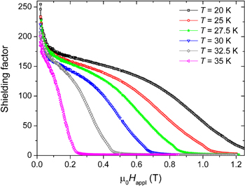
Figure 4. SFs measured in the axial field configuration at the tube's centre (position z1), as a function of the applied field and for temperatures ranging from 20 to 35 K.
Download figure:
Standard image High-resolution imageRemarkably, SFs higher than 175 and 55 were found at T = 20 K and μ0Happl = 0.1 T and 1.0 T, respectively.
Since in practical applications the shield's axis is seldom perfectly parallel to the applied field direction, we also investigated the shielding performance of the tube when the external field is applied perpendicular to its axis. In figure 5, Bz measured at T = 25 K along the tube's axis as a function of the cycled applied field and the corresponding SFs are plotted, whereas figure 6 shows the SFs measured in the tube's centre (position y1), for temperatures ranging from 20 to 35 K. As expected [28], in this configuration a worse field mitigation occurs. However, SFs higher than 4.6 and 4.3 are still achieved at μ0Happl = 0.1 T and T = 20 and 30 K, respectively.
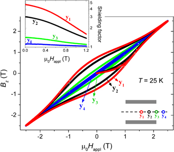
Figure 5. Magnetic induction measured at T = 25 K by the four Hall probes positioned along the tube's axis as the applied field was cycling (main frame). The measurement was performed in the transverse field configuration. In the inset the SFs are plotted.
Download figure:
Standard image High-resolution image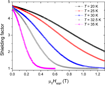
Figure 6. Shielding factors measured in the transverse field configuration at the tube's centre (position y1), as a function of the applied field and for temperatures ranging from 20 K to 35 K.
Download figure:
Standard image High-resolution image4. Modelling
4.1. Analytical model for critical current density evaluation
The critical current dependence on magnetic field is tipically evaluated by the magnetization hysteresis cycle performed on small samples cut from the bulk. However, the so-estimated Jc could not give a correct evaluation of the macro-Jc flowing in the whole bulk [20].
Here, taking advantage of the tubular geometry of the sample we calculated Jc from the magnetic induction cycles as proposed by Bartolomé et al for finite superconducting rings [25]:
where  is the induction cycle width measured at a given applied field in the axial field configuration and the function f provides the dependency of Jc on the geometry of the system:

with Ro and Ri being the outer and inner radii of the tube, respectively, and h the tube height and z the distance from the tube centre (i.e. z = 0 corresponds to position z1 in figure 2(a)).
4.2. Numerical model for computation of the magnetic induction
To simulate the magnetic properties of the superconducting tube we used a vector potential formulation based on Campbell's numerical method [29] in the form proposed by Gömöry et al [30], which we already successfully applied in previous studies on MgB2 and hybrid superconducting/ferromagnetic systems [22, 31]. All the calculations were done by a commercial finite-element software [32].
Here, we focus on the axial field configuration. Exploiting the axisymmetric geometry of the problem, we worked in cylindrical coordinates. Consequently, the vector potential has only one component,  being r the radial coordinate and uϕ the unit vector along the ϕ direction, and the current density flowing in the superconductor is defined by the equation:
Here Aϕ,p (r, z) is the local value of the vector potential achieved in the previous step of change of the applied field, An is a scaling factor affecting the shape of the current distribution inside the superconductor (here assumed to be equal to 5 × 10⁻⁸ Wb m−1 [22]) and jc is the local current density. In the hypothesis that the magnetic flux penetrates/exits monotonically from the sample surface when the applied field increases/decreases monotonically, we set Aϕ,p (r, z) = 0 and Aϕ,p (r, z) = Aϕ,max (r, z) in calculating the first-magnetization curve and the second branch of the magnetic induction cycle, respectively. Aϕ,max (r, z) is the vector potential distribution obtained when the maximum external field is applied. Finally, the dependence of jc on magnetic field is taken into account starting from the fit of the experimental Jc curve obtained by equation (1).
The magnetic induction field is invariant under a rotation around the z-axis and has no ϕ-component:  being ur and uz the unit vectors along the r- and z-directions, respectively.
The source term for the magnetic field is represented through the boundary conditions: at a large distance from the sample, the field is assumed to be constant, equal to μ0Happl and applied parallel to the tube's axis.
5. Critical current density evaluation and comparison between experiment and simulation
Figure 7 shows the Jc curves obtained from the B versus μ0Happl cycles for temperatures ranging from 25 K to 35 K by applying equation (1). They are evaluated averaging the critical current densities obtained separately from the magnetic induction cycles measured by the four Hall probes. Remarkably, these Jc values differ by less than 5% proving the sample homogeneity. Due to the flux jumping phenomena [33, 34] we could not measure the return branch of the magnetic induction loops at 20 K.

Figure 7. Jc dependence on the applied magnetic field obtained from magnetic induction cycles measured at different temperatures (symbols). The solid lines are the fits of Jc curves by equation 3 in the high-field range (i.e. applied fields higher than the full penetration field in the virgin branch of the hysteresis cycles).
Download figure:
Standard image High-resolution imageIn order to reproduce the experimental Bz data by simulation, the Jc curves reported in figure 7 were fitted by a polynomial law and the so-obtained Jc dependence on magnetic field was inserted in equation (2). The comparison between experimental and computed magnetic induction fields at T = 25 K is reported in figure 8 (only for the Hall probe at the tube's center, for clarity). The agreement is good only in the range of high magnetic fields, i.e. approximatively above the full penetration field in the first- magnetization curve. When the field is low, significant differences between experimental and computed curves emerge. This result is confirmed at the other investigated temperatures and for the other Hall probes positions. It suggests that an approach only based on applying equation (1) is not suitable to calculate the critical current density at low fields. This could be attributed to the fact that the approach described in section 4.1, starting from the hypothesis of the Bean model [35], assumes a constant critical density. Indeed, as it was demonstrated by Chen and Goldfarb [36], the Bean model can be inadequate, or even misleading, to estimate the critical current density at low applied fields when the superconductor magnetic moment strongly depends on Happl.
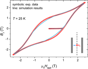
Figure 8. Comparison between the magnetic induction cycle measured at T = 25 K by the Hall probe located in the tube's centre and the corresponding cycle computed using a polynomial interpolation of the experimental Jc curve reported in figure 7.
Download figure:
Standard image High-resolution imageThus we decided to insert a jc(B) dependence that could reasonably describe the real behavior also at low fields into equation (2). Starting from the magnetic field dependence of Jc found by Fujishiro et al [37] we fitted the portion of each curve reported in figure 7—just in the range of applied fields higher than the full penetration field—by the following exponential relation:
where Jc,0, B0 and γ are the fitting parameters. Their values are summarized in table 1 for all the investigated temperatures.
Table 1. Fitting parameters obtained by fitting the critical current densities plotted in figure 7 by equation (3). As detailed in the text, the fits were carried out just in the high-field range.
| T | Jc0 (A m−2) | B0 (T) | γ |
|---|---|---|---|
| 25 K | 4.68 × 10⁸ | 1.30 | 2.29 |
| 27.5 K | 3.80 × 10⁸ | 1.06 | 2.38 |
| 30 K | 3.01 × 10⁸ | 0.83 | 2.52 |
| 32.5 K | 1.92 × 10⁸ | 0.58 | 2.77 |
| 35 K | 0.93 × 10⁸ | 0.31 | 2.76 |
Then, assuming that the critical current density dependence on magnetic field can be described by equation (3) in the whole investigated field range, we introduced it in equation (2).
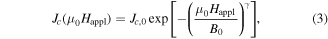
This procedure provided an excellent agreement between the experimental and computed data, as evidenced in figure 9 where magnetic induction fields obtained from finite-element modelling at different positions/temperatures are shown as solid lines superimposed to experimental results. This agreement indicates that the critical current density chosen for the simulations allows a reliable estimation of the induction field measured experimentally. Therefore the chosen modelling approach well predicts the performance of the shield.
Figure 9. Comparison between the magnetic induction fields (a) measured by the four Hall probes at T = 25 K (symbols) and the corresponding cycles computed by numerical simulations (lines) and (b) measured by the Hall probe located in position z1 at different temperatures (symbols) and the corresponding cycles computed by numerical simulations (lines).
Download figure:
Standard image High-resolution image6. Wall thickness and cap addition influence on the shielding performances
Since the modelling approach has been validated by the comparison to the experimental data, we can use it to drive the design of future shields with similar aspect ratio but improved shielding performances. With this aim, we evaluated numerically how changes in size and shape of the original tube affect its SF. To do this, we calculated and compared the magnitude and the profile of the SF at several positions (y, z) inside the screens. All the simulations were performed assuming the working temperature of 25 K and external fields applied parallel to the shield's axis.
An improvement in the screening performance of hollow cylinders was predicted by increasing their lateral wall thickness [38]. However, previous works on long tubular shields by Willis et al [39] and Niculescu et al [40] evidenced that the Jc(B) dependence influences the flux penetration rate in the shield's wall with raising the external field. In our case, due to the geometry of the sample, magnetic flux also enters the shield via the tube's apertures. Therefore, at least at lower applied fields, the wall thickness is expected to affect the shielding properties in a non-remarkable way. Numerical simulations confirm this assumption. In figure 10 we plotted the SFs calculated at μ0Happl = 0.5 T for four different thicknesses of the tube's wall, obtained varying its external radius. Against an increase of about 60% of the shield's mass (corresponding to a 50% increase of the outer radius) a SF improvement of about 30% is just achieved. Similarly, a negligible SF reduction occurs when the outer radius is lowered by 16%.
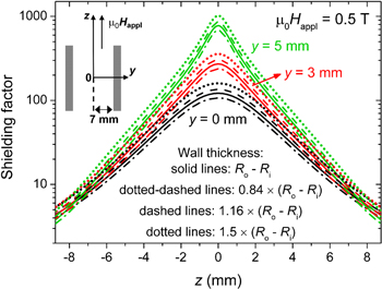
Figure 10. Comparison among the shielding factors calculated as a function of the z-coordinate (i.e. parallel to the tube's axis) at different radial positions (y-coordinate) and assuming four different wall thicknesses of the tube. The zero position corresponds to the centre of the tube. The simulations were carried out imposing the axial applied field μ0Happl = 0.5 T.
Download figure:
Standard image High-resolution imageNoticeably, these simulations highlight the occurrence of a peak in the SFs at a radial distance of about 4–5 mm from the tube's axis, where SF values up to 103 are predicted already for the original tube.
Based on previous investigations, two approaches are expected to provide more promising improvements in screening performances: closing the tube by means of a superconducting cap [2, 41] and/or adding ferromagnetic sheets [31, 42]. Here, we focus on the former method. The latter, which requires the simultaneous modelling of both the superconducting and ferromagnetic materials, will be investigated elsewhere.
By means of the fabrication technique described in section 2:
- (i)cup-shaped shields [15] can directly be fabricated from a bulk cylinder. In this case the tube and its cap are joined by means of a superconducting joint and the supercurrents can flow across the interface;
- (ii)the cap can be produced separately and just placed on the tube.
Firstly we investigated the former situation (i). Three closures were analysed: a disk-shaped-cap and two hollow-disk-shaped-caps with two different inner diameters, as sketched in figure 11. Note that the presence of a hole in the cap can be exploited for electric wiring or as a window for a sensor located in the shield. The external diameter and the thickness of the cap were always 20.3 and 3 mm, respectively (i.e. equal to the external diameter and to the lateral wall of the original tube, respectively).
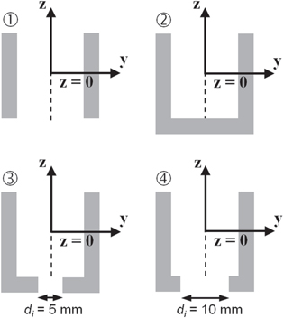
Figure 11. Schematic view of the shield geometries used in the simulations. Layout no. 1 corresponds to the tube characterized experimentally (h = 17.5 mm, Ro = 10.15 mm, Ri = 7 mm). Layouts no. 2–4 were obtained by adding a 3 mm thick cap to layout no. 1: their inner depth is equal to the height of the tube. The zero position always corresponds to the centre of the starting tube.
Download figure:
Standard image High-resolution imageFigure 12 compares the SF profiles computed inside the tube characterized experimentally (layout no. 1) with those obtained by closing the bottom aperture of the tube (layouts no. 2–4) for the axial applied fields μ0Happl = 0.1, 0.5 and 1.0 T. In all the cases the cap addition strongly reduces the magnetic flux penetration from the bottom aperture of the tube and a remarkable enhancement of the SF is observed, even reaching 105 at μ0Happl = 0.5 T when a non-holed cap is designed. As expected, the presence of a hole in the cap induces a worsening of the SF: reductions of about three and two orders of magnitude are observed near the closure for the 10 and 5 mm large holes, respectively, along the shield's axis (i.e. at the radial coordinate y = 0). However, for the narrower hole this reduction is completely recovered when moving toward the lateral wall of the vessel.
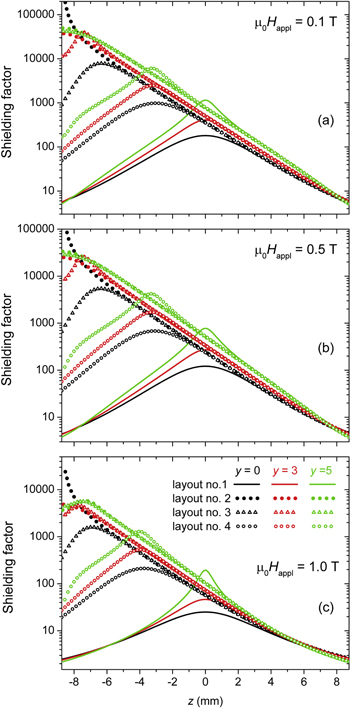
Figure 12. Comparison among the SFs calculated for the layouts no. 1–4 as a function of the position along the z-axis (coordinate y = 0) and other two parallel axes at radial distances y = 3 mm and y = 5 mm. Simulations were carried out assuming axial applied fields μ0Happl = 0.1 T (a), 0.5 T (b) and 1.0 T (c). The zero position always corresponds to the centre of the starting tube (see figure 11) and a superconducting connection between the tube and cap is always supposed.
Download figure:
Standard image High-resolution imageAfterwards, layouts no. 2–4 were modified assuming that the cap is just placed at the bottom of the tube without any conducting joint (situation (ii)). To take into account the possible roughness of the two surfaces in contact, a 0.2 mm large air-gap was added between the tube and the cap. The presence of this gap does not modify the shielding ability at low fields as it is clearly visible in figure 13(a), which reports the SF radial profiles calculated 0.25 mm above the cap when an axial field μ0Happl = 0.5 T is applied.

Figure 13. Comparison among the SFs calculated for the layouts no. 2–4 as a function of the position along the radial direction at the coordinate z = −8.50 (corresponding to a distance of 0.25 mm above the cap). Black symbols refer to layouts with superconducting joint, while cyan symbols refer to layouts where an air-gap of 0.2 mm occurs between the tube and the cap. Simulations were carried out assuming axial applied fields μ0Happl = 0.5 T (a) and 1.0 T (b). The zero position always corresponds to the axis of the shield (see figure 11).
Download figure:
Standard image High-resolution image
Conversely, when the applied field exceeds 0.9 T, the magnetic flux penetration from the lateral gap becomes significant. A gradual increase occurs in xy-plane for the air-gap-effect with increasing the distance from the shield's axis (figure 13(b)).
7. Conclusions
We investigated the shielding properties of an MgB2 tube using both experimental characterizations and numerical simulations. The tube was produced via an innovative technique, namely spark plasma sintering and machining, which allows obtaining fully machinable MgB2 bulks with desired sizes and complex shapes.
The ability to mitigate an external magnetic field was checked as a function of temperature, applied magnetic field and position, in both axial and transverse field configurations. Although the height/outer radius aspect ratio of the tube is only 1.75, the shielding factor measured in the tube's centre at 20 K, when the axial field μ0Happl = 0.1 T is applied, is higher than 175 and still exceeds 120 at T = 25 K and μ0Happl = 0.5 T.
Experimental results in the axial field configuration were well reproduced by numerical simulations using a modelling approach based on vector potential formalism. Notably, the Jc(B) characteristics introduced in the model were directly obtained by means of a two-step procedure from the magnetic induction field cycles measured with Hall probes.
This modelling approach also proved that only limited SF improvements are achievable by increasing the wall thickness of the tubular shield. Conversely, new layouts consisting in cup-shaped vessels or obtained simply by placing a cap on one of the tube's apertures are expected to lead to SFs of up to 105 and 104 at T = 25 K and in axial applied fields μ0Happl = 0.1 and 1.0 T, respectively.
To complete the study of these shielding solutions and to optimize their designs under realistic operation conditions, predictions of their screening properties for various orientations of the applied magnetic field are necessary. This analysis would benefit from the present modelling approach, even though it requires a full 3D description [43, 44].
Acknowledgments
We wish to thank F Gömöry for fruitful discussions. Romanian team acknowledges MCI-UEFISCDI, grant POC 37_697 no. 28/01.09.2016 REBMAT and Core Program 2017/2018. VB and MT acknowledge support from the project 'Departments of Excellence' (L. 232/2016), funded by the Italian Ministry of Education, University and Research (MIUR).