
Abstract
We present a model for streamer coronas emerging from a spherical electrode at high electrostatic potential. By means of a macroscopic streamer model and approximating the corona as a set of identical streamers with a prescribed spatial distribution around the electrode, we establish that coronas more densely packed with streamers are slower and more efficient at screening the electric field inside the streamers. We also apply our model to investigate the electrostatic potential at the boundary of the corona sheath that surrounds a leader and we underline the relevance of the rise-time of the leader potential during a leader step.
Export citation and abstract BibTeX RIS

Original content from this work may be used under the terms of the Creative Commons Attribution 3.0 licence. Any further distribution of this work must maintain attribution to the author(s) and the title of the work, journal citation and DOI.
1. Introduction
When a sharp electrode such as a needle or a wire is subjected to a high electric potential it ignites a type of electrical discharge called corona. Depending on conditions such as electrode geometry and rise time of the potential, the discharge may exhibit a variety of forms [1, 2]. A sufficiently sharp electrode on which a sufficiently impulsive potential is applied launches a corona composed of many thin filaments called streamers that propagate due to electron impact ionization in a high-field volume around their tips [3–5].
Streamer coronas exist on Earth in a variety of natural and artificial conditions. They appear as sprites [6, 7] or blue jets [8–11] on the upper atmosphere and they form a sheath around the hot, highly conducting leader core of a long spark [12] or an advancing lightning channel [13]. In artificial electrical systems, the undesired emergence of coronas can cause severe negative effects like power loss or high-frequency electromagnetic interferences. On the other hand, streamer coronas have a variety of beneficial applications such as water and gas cleaning, electrostatic precipitation, ozone creation, or even inactivation of bacteria (see e.g. [14, 15]).
Single streamers have been widely studied from a microscopical standpoint with Monte Carlo [16–18], fluid [19–25], and hybrid [26] models. Other studies on specific phenomena like branching [27, 28], head-on collisions between streamers [18, 23, 29, 30], the effect of inhomogeneities of the medium [31, 32] or the formation of luminous structures inside the channels [33, 34] are also available. The interaction between streamers, however, is a very complex matter and most of the works about it involve only two streamers [35–39]. Up to our knowledge, only the works by Naidis [35], Akyuz et al [40] and Luque and Ebert [41] have simulated a system with more than two streamers, and in all cases the underlying system was heavily simplified.
Recently we presented a macroscopical model for streamers treating them as advancing imperfect conductors [42]. This model allowed us to explore long term channel properties like channel inhomogeneities and their role in the formation of streamer glows. Here we apply our model to investigate the properties of streamer coronas composed of many interacting streamers emerging from a spherical electrode. Our aim is to understand how properties of the corona depend on the density of streamers that compose it. As we see below, the corona model presented here is considerably simplified but precisely for that reason it serves to build an intuition about the corona's complex dynamics.
This paper is structured in six sections, the first being this introduction. In section 2 we describe both the single streamer and the streamer interaction model, explaining the underlying assumptions and approaches. In section 3 we describe the numerical approximations and the implementation of the model. In section 4 we describe the results obtained in our simulations for one configuration of experimental interest whereas in section 5 we investigate the potential drop within a corona. Finally, in section 6 we summarize the conclusions of our work.
2. Model description
In this section we start by briefly summarizing the streamer model used as base for the streamer corona. Then we explain how to add the interaction between several streamers and the numerical implementation used in this work.
2.1. General description of the single streamer model
We start with a brief description of the main equations and assumptions of the single streamer model, as thoroughly described in [42]. The streamer is modeled as a symmetric one-dimensional imperfectly conducting charged channel attached to an spherical electrode of radius a and propagating in the z direction (see figure 1(a)). This system evolves according to electrodynamic and chemical models that are coupled through the electric field inside the streamer channel.

Figure 1. Model geometry of the simulations with (a) a single streamer and (b) two identical interacting streamers, S0 and S1.
Download figure:
Standard image High-resolution imageThe transport of charge within the channel is determined by charge conservation ∂tq = −∇ · j, where q is the charge density and j the current density. Integrating this equation across a plane Γ perpendicular to the streamer channel we obtain

where λ is the linear charge density, and I is the current intensity:

Under the assumptions of negligible electron diffusion, independence of mobilities from the electric field, and uniform charge-carrier densities across the channel, the current intensity is proportional to the integral of the electric field on the section of the streamer and (1) becomes a linear differential equation. The intensity I is composed of three terms, I = Iself + Ibg + Isurf, that model the electric self-interaction of the streamer, the influence of an electrode and background field, and the effect of the surface current around the streamer head as it propagates. This expression assumes that the streamer radius is sufficiently small that charge transport in the transversal direction is instantaneous and we can describe it using a linear charge density λ.
The terms Iα, where α ∈ {self, bg, surf}, can be expressed in an integral form for each z in the streamer:

where σ(z) is the conductivity of the streamer,  0 the vacuum permitivity, and
  the kernel describing the influence on z of the charges in
  .
.
The chemical model contains 17 species coupled by 78 reactions, as described in [42]. It boils down to a system of ordinary differential equations describing the evolution of the densities  of each charge carrier si, i ∈ {1, ..., nspec} according to a set of reactions rj, j ∈ {1, ..., nreac}. The equation governing the evolution of each species si is given by:
where Ai,j is the net number of molecules of species si created each time reaction rj occurs (given by a difference on the stochiometric coefficients in rj), kj is the rate coefficient of reaction rj, and I(j, l) is the index of the reactant l of reaction rj. The rate coefficients kj, j ∈ {1, ..., nreac} are functions of the local electric field, which in [42] is approximated by the field at the axis for each z. As we explain in section 3, in this work we approximate instead the local field at each z by the average of the field on the disk perpendicular to the streamer.
The propagation velocity of the streamer depends on the streamer radius R0 and the field at the tip (estimated immediately outside the streamer, since it is discontinuous at the tip) following the expression derived by Naidis [43]. This expression is a relationship between the streamer radius, its velocity and the background electric field. A nonlinear root finder can be used to solve for the velocity given the other two quantities. The main assumption behind Naidis' formula is that the electron density undergoes multiplication by a fixed factor within the area around the streamer head where the electric field is above breakdown. For positive streamers, the generation of a sufficient quantity of electrons outside this active area due to photo-ionization is implicitly assumed in the derivation.
The model includes the effect of the field ahead of the streamer tip by imposing densities  at the streamer tip, as explained in [42]. Since streamers are initiated with a finite length, the species densities are given initial conditions inside the streamer body, which we set also as
  .
.
2.2. Additional streamers
Let us now consider the effect of additional streamers on the model. Neighboring streamers influence each other directly through their electrostatic interaction; to incorporate this in our model we introduce two assumptions, in addition to those in [42] and described in section 2.1:
- There is a perfectly symmetrical configuration of streamers around a spherical electrode of radius a, so we can consider that all the streamers are equal, i.e. that the length, density charge, and other characteristics of all the streamers Si, i > 0 are the same as those of S0. This allows us to concentrate on only one streamer, S0.
- The streamer radius R0 is small compared to the minumum distance between streamers. This assumption allows us to approximate Si, i > 0 as an infinitely thin line of charge when we calculate its effect on S0. Furthermore, we also neglect the variation within the cross-section of S0 of the electric field created by Si. To summarize: we consider the finite width of the streamers only for the interactions between separate points of the same streamer but not for the interaction between different streamers.
The geometry of the effect exterted on S0 by a neighboring streamer S1 is sketched in figure 1(b). We calculate the electric field at a point p0 on streamer S0 which, without loss of generality, we consider to be on the z axis. Thus, p0 = (x0, y0, z0) = (0, 0, z0) ∈ S0. As in [42], we only need the z component of the electric field induced in p0 by a point charge q1 located at p1 = (x1, y1, z1) ∈ S1. This is:

Now, given that  , where
  is the α component of the unit vector in the direction generating S1, and l1 is the distance from p1 to the origin, (5), can be rewritten as:
Then the contribution of the whole streamer S1 is:
where λ1 is the linear charge density in S1.
Now, the electric current generated in the disk of S0 at z0 is:

where, as in [42],  is a smooth function that models the variation of the radius along the streamer channel.
Since all the streamers are identical we drop the subscripts in l, λ, and σ and, for each streamer Si, i > 0, define a kernel
Following the method of images, we add a virtual charge  (called image or mirror charge) to satisfy the boundary conditions in the spherical electrode boundary. We need, then, to add the effect of
  located at a distance
  . Since
  , and
, and  with κ = a/l being a squeeze factor, we derive the mirror kernel for each streamer Si with i > 0:

From Ki and Km,i we can define a kernel Gi so the contribution of streamer Si to the current intensity in z0 ∈ S0 has the form of (3). Adding up all kernels we obtain the following expression for the total current intensity I at each point z0 ∈ S0:

where Gtot is a kernel that now includes the self interactions of streamer S0, the background and surface current, and the contributions of all the surrounding streamers Si, i = 1... n, that is,  .
.
3. Numerical implementation
We use finite differences to solve the partial differential equations from section 2. We apply a leap frog scheme to couple the electrodynamical and the chemical parts of the model, and a Crank–Nicolson discretization for both equations (1) and (4). Figure 2 shows the flowchart used to implement the calculations. At each time t the streamer length is discretized in a set of cells Ci, i = 1... L with boundaries zi±1/2, where the right boundary of cell L is ztip. In the electrodynamical step ztip moves forward with a velocity obtained from the expression derived by [43] and we solve the charge transport system. Some variables describing the system, like conductivity, densities and electric field are defined at cell boundaries (e.g. σi±1/2), while the charge density λi is considered constant within each cell i:

where qi is the total charge in the cell and Ii±1/2 are the current intensities at the boundaries. The current intensity at the boundary of cell j is given by (11), which we integrate numerically in each cell. This way, we can define an interaction matrix M = {mij}, and the background component vector b = {bi} so at each time t the current intensity at the rightmost boundary of cell i is
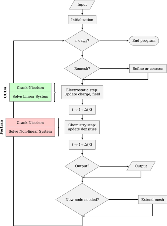
Figure 2. Flowchart of the corona model. Calculations in the electrodynamic step accelerated with CUDA are marked in green, while Fortran accelerated calculations in the chemical system are marked in pink.
Download figure:
Standard image High-resolution imageFor the single streamer model, each element mij from the interaction matrix is the cross-sectional current induced at the boundary of cell i by an unitary charge in cell j, and each element bi is the current induced at the boundary of cell i by the background and electrode field. In this corona model, the interaction matrix includes also the effect of the jth cell from all the other streamers. With this expression, we cast (12) as a subtraction of interaction matrices and background vectors forming a linear system.
The electrodynamical system is particularly apt for parallelization, since each element of the interaction matrix can be calculated independently. We have, thus, accelerated its performance using CUDA (integrated with python using pyCUDA). As for the chemical processes, the discrete system to solve is sparse and nonlinear, and we solve it iteratively, using Newton–Raphson. The solution of this system is accelerated using Fortran and OpenMP.
Our previous work [42] showed that, in the conditions of the model, the electric field at each point z of the streamer, used to couple the electrodynamic and chemical parts of the model, could be approximated by the field at the axis. We have found that the goodness of this approach decays when we increase the number of streamers. For this reason in this work we instead calculated an average electric field across the channel.
One point where we still need to calculate the field at the axis is at the tip. The field at the axis in the single streamer case is calculated using an expression analogous to (3) with a different kernel Gax:

where
To calculate the influence of a streamer Si on the field at the axis in z0 ∈ S0, we derive a kernel Gax,i from (7),

This expression can be combined with (14) to obtain the final expression for the field at the axis for z0 ∈ S0:
When z0 = ztip, the integral of the field at the axis (17) is bounded and, thus, convergent, but for z → z0 the convergence order is increasingly large as z0 approaches ztip. We evaluate the field at a point slightly beyond the actual tip z0 = ztip + εtip, where  with ntip an order factor (typically 3). This ensures that we use an appropriate εtip, close enough to represent the field at the tip, but far enough that the resolution needed for the field estimation is reduced. Even after this, we had to use resolutions of the order of 105 to obtain results with enough precision, so additional optimization was needed. We added a variable change to expand the integration domain in the tip cell, so with our new variable ξ, the field slope is not too steep. The usual ξ = z−n variable change helped but not enough so we opted for a variable change capturing the decay of the radius close to the tip. We used the following expression:

which is the inverse of the smoothing decay factor applied to the radius near the streamer tip,  . The variable change in (18) allowed us to use the same resolution as in the rest of the streamer, heavily accelerating the code while ensuring that a good and robust approximation of the field at the tip is being used.
One final element in our model is the distribution of n streamers in the spherical surface of the electrode. One possibility is to distribute them randomly with a constant density per unit surface. However this often leads to pairs of streamers that are too close and that in reality would merge into a single one. Therefore we look for a distribution of inception points that in some sense maximizes the minimum distance between them, accounting for the repulsion of streamers as well as for the possibility of merging.
The distribution of points on the surface of a sphere that maximizes the minimum distance between points is a classical open problem (see e.g. [44]), described as one of the problems of the century by Smale [45]. The configurations of points solving this problem are called spherical codes and have different applications depending on the metric considered. Given the electrostatic nature of our problem we opted for the so called Thomson problem (as described in e.g. [46]), which aims to determine the equilibrium positions of classical electrons on the surface of a sphere, subject to their electrical repulsion. This problem has been solved exactly for some numbers of particles, where the equilibrium positions are the vertices of classic platonic solids and the distance between particles is constant. However, these perfectly symmetrical configurations limit significantly the number of streamers we can use, so we use quasi symmetrical approximate solutions found numerically. In this work, we use the database of solutions computed by [47], which we apply to the distribution of streamers on the electrode surface. We will use configurations with n = 50, 100, 200, 400 streamer inception points, shown in figure 3.
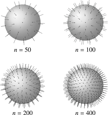
Figure 3. Configurations of n = 50, 100, 200 and 400 streamers in a spherical electrode following a Thompson distribution.
Download figure:
Standard image High-resolution image4. Results
In this section we describe the results obtained in a configuration which has similarities to laboratory conditions, although the need of symmetry of our model makes it impossible to recreate exact experimental configurations. All the initial conditions and simulation parameters are shown in table 1: we consider a positive streamer corona emerging from a spherical electrode that is live with a potential of 50 kV. The electrode radius is 2 cm, resulting in mean streamer separations at the electrode's surface varying from about 3.5 mm to about one centimeter, as reflected in table 2. Since our model does not account for streamer inception, we have to initiate the streamers already with a finite length, which we chose as 1 cm.
Table 1. Simulation parameters for the positive corona emerging from a spherical electrode.
| Variable | Value | Units |
|---|---|---|
| Electrode radius, a | 2 | cm |
| Electrode potential, V | 50 | kV |
Electron density at the tip, 
|
1020 | electrons m−3 |
| Streamer radius, R0 | 1 | mm |
| Streamer initial length | 1 | cm |
| Background chemistry | humid air | — |
| Pressure | atmospheric | — |
| Final time | 10 | ns |
Table 2.
Density of streamers at the electrode and approximate mean distance between them when considering a spherical electrode of radius  . The density is d = n/4πa2 and the mean distance is d−1/2.
| Number of streamers, n | Surface density | Average separation |
|---|---|---|
| 50 |

|
10 mm |
| 100 |

|
7 mm |
| 200 |

|
5 mm |
| 400 |

|
3.5 mm |
4.1. Propagation of a single streamer compared to a streamer inside a corona
Before describing the outcome from the many-streamers model let us briefly summarize the results obtained with our model for single streamers [42]. In figure 4 we plot the electric field created by a single streamer advancing from an electrode with the initial conditions from table 1. The plot shows the electric field against the streamer length for all recorded times, where time is indicated by a color scale. The initial field of the streamer is that of the electrode, and it is screened in the interior of the streamer channel. The field at the tip increases with time, and when it is sufficiently high, the tip of the streamer starts advancing. The propagation, in turn, softens both the screening in the streamer channel and the increase of the field at the tip. Increasing the potential of the electrode, the leading ionization, or the radius of the streamer channel will lead to faster propagation.

Figure 4. Time evolution of the electric field in the streamer channel against z. The left panel shows the results for the simulation with a single streamer and the right panel shows the results for a simulation of a corona with 200 streamers distributed as explained in the text. Different colors show the electric field at different times, according to the colorbar.
Download figure:
Standard image High-resolution imageThe right panel of figure 4 shows the evolution of a symmetrical corona with 200 streamers with the same initial conditions (see table 1) as the single streamer model. Qualitatively, the general evolution of the streamer is similar regardless of the number of streamers: screening of the field in the streamer channel and increase of the field at the tip, which triggers propagation. Quantitatively, however, the effect of the additional streamers in the corona stands out when we compare both panels from figure 4: the additional streamers contribute to a better screening of the electric field and lead to a lower electric field at the tip. The corona with 200 streamers, in figure 4, shows a field inside the channel approximately an order of magnitude lower than in the single streamer case. The field at the tip is also lower for 200 streamers although the differences are less than a factor 2. These differences are enough, however, for the total propagation distance to be substantially smaller, around a factor 6.
4.2. Dependence on the streamer density
Now that the general evolution of the streamer corona has been described let us generalize our results to a varying density of streamers. Figure 5 shows the status of simulations with different amounts of streamers at final time,  .
.

Figure 5. Electric field (top left panel), charge density (top right panel), and electron density (bottom left panel) against length at final time ( ). Each color in each plot represents the simulation of a corona with a different number of streamers, as shown in the legend in the bottom right panel. Note that the maximum electron density (indicated here by a dashed line) is an input parameter of our model.
Download figure:
Standard image High-resolution imageThe top left panel of figure 5 shows the electric field in the streamer channel for coronas with 1, 50, 100, 200, and 400 streamers, each shown in a different color. In all the simulations, the field shows a similar profile to that of a single streamer, which is to be expected given that due to the symmetry in our corona, all the streamers in the simulation behave as streamer S0 (as explained in section 2). Even with these assumptions, the effect of additional streamers in the corona is clear: the electric field decreases as the number of streamer increases, both the peak field and the field along the streamer channel. Since the streamer velocity increases with a higher field at the tip [43], as the number of streamer increases, the propagation velocity decreases. This is summarized in figure 6, where we plot the mean velocity of coronas with varying number of streamers.

Figure 6. Streamer mean propagation velocity against number of streamers.
Download figure:
Standard image High-resolution imageA special case is the simulation with n = 400 streamers. In this case the streamers barely propagate at all within 10 ns because the electric field at the tip is too low for sustained streamer advance. What this case tells us is that there is limit for the density of streamers in a corona imposed by electrostatic considerations. In our case the maximum number of streamers was about 400 but this quantity depends on the electrode potential and radius. Likely, the state in which a perfectly symmetrical distribution of many streamers stops is physically unstable and, due to small differences in the length of the streamers, an actual corona would continue its propagation with a lower density as a result of leaving behind the shortest streamers.
Turning back to figure 5, its upper right panel shows the charge density in the streamer channel against streamer length at final time for the same simulations with the same code color as the upper left panel. For simulations with n < 400, the charge density increases with z, but the peak is reached within the streamer body, slighly before the streamer tip, where it decreases as it is invested in streamer propagation. The charge density in the simulation with 400 streamers decreases near the electrode and then steadily increases with z, reaching the peak at ztip. In general, the charge density is lower as we increase the number of streamers, both the peak and near the electrode. However, the positive slope of the charge density increases with n.
The lower left panel from figure 5 shows the electron density in the streamer channel against z. For the simulations with significant propagation, n < 400, the electron density increases with z, and the peak is reached at the tip, where the leading electron density is  as per our boundary condition. Both the electron density near the electrode and its slope decrease with increasing n.
The observations detailed in this section lead us to the first and main conclusion of this work: the higher the density of streamers in a corona, the slower is their propagation and the lower is their internal field. To understand this principle let us consider two configurations with different streamer densities d1 and d2 with d1 < d2. Suppose that at a given time the single-streamer charge density is the same in both configurations. In the configuration with d2 the electric field is more screened due to the neighboring streamers. Since this implies a lower current, after some propagation it leads to a lower charge density. Therefore in general the charge density per streamer is lower in dense coronas. Since the electric field at the tip of each streamer results mostly from this charge density, the propagation of dense coronas is also slower. This process is combined with another principle described in [42]: slower streamers have lower internal electric fields. These lower electric fields in our case explain the depletion of electrons observed in the lower panel of figure 5: this is due to three-body attachment, which is more efficient for lower fields.
4.3. Electric field screening
Let us now focus on the evolution at a fixed point in the streamer channel. Figure 7 shows the electric field (top panels), and the electron density (bottom panels) for two fixed points in the streamer. We chose  (left panels) and
  (right panels), which are the two extremes of the streamer at initial time. From a qualitative standpoint, all the points in the streamer channel have an evolution similar to that of the electrode boundary, and all the points beyond the initial length of the streamer that are reached by it will behave in a similar fashion to the initial tip.

Figure 7. Electric field (top panels), and electron density (bottom panels) against time at fixed z. The left plots show the variables at  , the electrode boundary, while the right plots show the results for the initial tip of the streamer,
  . Each color in each plot represents a simulation with a different number of streamers, while the rest of the initial parameters are those in table 1.
Download figure:
Standard image High-resolution imageThe top panels of figure 7 show the electric field at the electrode boundary  (top left panel), and at the initial tip
  (top right panel). At the electrode boundary, in coronas with any number of streamers, the electric field initially decays at a rate that is faster for higher streamer densities. For n < 100 the field remains quasi stationary at the minimum value, but for denser coronas the field slightly increases with time, with a steeper slope for larger amounts of streamers. At
  , which initially is the tip of the streamer, the field increases until a value close to
  is reached, and then the streamer expansion starts and the field decreases. The evolution of the channel field, then, becomes similar to that of an inner point. The curves for the corona with 400 streamers are jagged due to its marginal propagation; as explained above this evolution is unstable and not to be expected in actual coronas.
In the upper-left panel of figure 7 we appreciate two clearly differentiated regimes for the streamer base: (a) a fast, roughly exponential, decay lasting for about 1 ns and (b) an approximately constant field afterwards.
The fast exponential decay (a) can be characterized by fitting the electric field decay to  , where the parameter τ represents the characteristic screening time. We applied this fit to times
  and the resulting parameters τ are plotted in figure 8. For comparison that figure also shows the dielectric relaxation time (sometimes also called Maxwell relaxation time) computed as τM = 0/σ, where 0 is the vacuum permitivity and σ the electrical conductivity. Figure 8 shows the Maxwell relaxation time using two approaches: with the inner channel conductivity as a red line, and with the average corona conductivity as a green line. For the average corona conductivity we have weighted the channel conductivity with the fraction of the surface covered by streamers,
  , where
  is maximum the radius of each streamer and
  is the radius of the electrode. Figure 8 shows that the dielectric relaxation time is a reasonably good approximation for this transitory regime, although it shows significant deviations for large streamer densities.
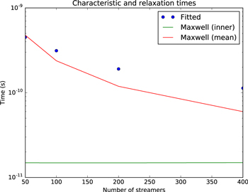
Figure 8. Characteristic decay times at the electrode boundary of the electric field (dots), and Maxwell relaxation time calculated from the conductivity, for the channel value in each streamer (red), and for the corona average (green) against number of streamers.
Download figure:
Standard image High-resolution imageRegime (b), which is more representative for the typical propagation of a streamer corona, sets in once the interior field is mostly screened. In that case there is a strong anti-correlation between high fields and high conductivities in the corona volume and therefore the dielectric relaxation calculated with a mean conductivity is a poor estimate for the evolution of the electric field. A careful investigation of this regime is beyond the scope of this paper and we leave it for a future work.
Turning back to figure 7, its lower two panels show the temporal evolution of the electron density at the two points that we considered. In both cases, the electron density decreases with time, although the decrease is larger when we approach the electrode. At any point in the streamer the depletion of electrons is faster as we increase the number of streamers in the corona. As explained above, this is due to the faster rate of three-body electron attachment at lower electric fields.
5. Potential drop within a streamer corona
As an impulsive corona propagates away from an electrode, it carries away part of the electrode potential. How efficiently this is performed depends on the strength of field-screening inside each of the streamers and, as we discussed above, this is heavily influenced by the streamer density in the corona. In this section we investigate this process.
The main motivation for this part of our study is the acceleration of electrons ahead of a lightning leader. This has been proposed as a mechanism for the generation of Terrestrial Gamma-ray Flashes (TGFs) [48, 49], which are intense bursts of energetic radiation connected to intra-cloud lightning processes [50, 51]. According to the thermal-runaway model of TGFs [52, 53], the high electric field at the tip of streamers pushes electrons from the bulk of the energy distribution into a runaway regime where they accelerate further and create relativistic-runaway electron avalanches (RREA) [54] in the electric field generated by a leader. A key magnitude in this process is the total potential available for the acceleration of electrons from the streamer tips to a position far-away from the leader [55].
Let us first consider the value of this potential in the simulations described above, where the electrode is at a potential  . The potential at the streamer tips is V1 = V0 − ΔV, where the potential drop ΔV is

with a being the electrode radius, and E(z) the electric field at a distance z from the center of the electrode.
The left panel from figure 9 shows the evolution of the potential drop at the corona boundary, calculated using (19). The right panel shows the drop at ztip at  against the number of streamers. As in section 4.3, we appreciate two regimes in the evolution of the electric screening: a fast decay from the background field where the corona acts as an average air conductivity followed by a proper corona where the potential drop increases with time. The key result here is that even with 50 streamers (an average separation between streamers of 1 cm at the electrode) the potential drop is less than 10% of the total potential. A higher streamer density implies even smaller potential drops. This means that almost the full potential of the electrode is transferred to the boundary of the corona.

Figure 9. Potential drop (V) between the electrode and the streamer tips. The left panel shows the evolution with time of the potential drop at the corona boundary, where colors indicate simulations with different n. The right panel shows the potential drop at the corona boundary and at final time  against the number of streamers.
Download figure:
Standard image High-resolution imageTo extend to our results to a situation closer to a lightning leader we run a simulation with the parameters listed in table 3. As our purpose is only to obtain a qualitative understanding of the corona dynamics around the leader, we mimicked the leader tip as a spherical electrode with radius 2 cm on which we apply a potential  with
with  and
and  . This dependence is an approximation to the rise of the potential at the leader tip after a leader step. Given the higher potential, we consider that the radius of the streamer is in this case 5 mm. We consider here n = 45 streamers, resulting in a density
  at the leader surface. These parameters approximate the characteristics of a streamer burst around a laboratory leader (see e.g. [56]).
Table 3. Initial conditions for the leader configuration.
| Variable | Value | Units |
|---|---|---|
| Number of streamers | 45 | — |
| Leader tip radius | 2 | cm |
| Potential rise time, trise | 100 | ns |
| Electrode (leader) potential, V0 | 1 | mV |
Electron density at the tip, 
|
1020 | electrons m−3 |
| Streamer radius, R0 | 5 | mm |
| Streamer initial length | 1 | cm |
| Background chemistry | humid air | — |
| Pressure | Atmospheric | — |
| Final time | 50 | ns |
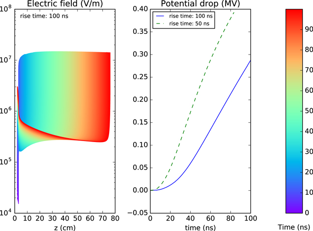
Figure 10 shows the results of the simulation. The left panel shows the electric field against z whereas the right panel shows the potential drop against time. When we compare the electric field with the configuration shown in figure 4, differences are obvious due mainly to the higher potential and the finite rise time. Initially, the channel field in the streamer from figure 10 is low, the initial potential being too low. Soon afterwards propagation starts and, due to the continuing leader potential increase, despite the screening inside the channel, the field at the leader boundary is significative. The field at the streamer tip remains below  due to the velocity of the streamer, which averages
  .
.
Figure 10. Left panel: Electric field against z color-coded for all times. Right panel: Potential drop (ΔV) at the corona boundary against time. This simulation was done with the initial conditions listed in table 3, simulating a corona around a leader tip.
Download figure:
Standard image High-resolution image
The right panel of figure 10 shows the potential drop at the corona boundary against time. Due to the increase in the leader potential, the streamers do not screen the field efficiently and at the end of the simulation,  , when the leader potential is
  , around half of that potential is spent within the streamer corona. An electron starting at the leader tip posseses around half of the leader potential available for acceleration.
With a finite potential rise time the electric field inside the streamers is established by the competion between screening and the increasing electrode potential. On the right panel of figure 10 we also show the potential drop of a simulation with a faster rise time  , which is significantly lower than that for
  . A proper comparison, however, has to take into account the different values of the streamer length and applied potential at a given time. In our simulations we found that the average inner field for
  stabilizes around
  V m−1 whereas for
  it reaches
  V m−1. This shows the relevance of the potential rise-time in the dynamics of streamers emerging from an electrode or a leader tip.
6. Conclusions
In this work we developed a macroscopical model for streamer coronas where, to allow for the simulation of many streamers, we simplified the corona as a symmetric configuration of straight streamer channels. Nevertheless, the model provides intuition about the effect of additional streamers on the overall evolution of the corona. It also provides semi-quantitative estimates of macroscopical corona properties. By means of this model we reached the following conclusions:
- As we increase the density of streamers in the corona, the screening of the field also increases. The electric field at the tip of the streamers decreases, which leads to slower streamer propagation for large numbers of streamers.
- Some macroscopical corona properties such as the timescale of electric field screening exhibit a clear collective behavior. These properties cannot be understood from the dynamics of a single streamer but rather derive from the interactions between many of them.
- The potential drop in a streamer corona is smaller for streamer coronas with larger amounts of streamers. To estimate the available potential for acceleration of electrons ahead of a leader corona we need to consider the rise time of the leader potential.
Further work on the modeling of streamer coronas should aim at removing some of the strongest simplifications in the present model. One particularly desirable objective would be to remove the unrealistical symmetry between all streamers and allowing different propagation speeds.
Acknowledgments
This work was supported by the European Research Council (ERC) under the European Union H2020 program/ERC grant agreement 681257 and by the Spanish Ministry of Science and Innovation under projects FIS2014-61774-EXP and ESP2017-86263-C4-4-R. This project has also received funding from the European Union's Horizon 2020 research and innovation program under the Marie Skłodowska-Curie grant agreement SAINT 722337. The authors acknowledge financial support from the State Agency for Research of the Spanish MCIU through the 'Center of Excellence Severo Ochoa' award for the Instituto de Astrofísica de Andalucía (SEV-2017-0709).