
Abstract
Objective. Positron emission tomography (PET) detectors providing attractive coincidence time resolutions (CTRs) offer time-of-flight information, resulting in an improved signal-to-noise ratio of the PET image. In applications with photosensor arrays that employ timestampers for individual channels, timestamps typically are not time synchronized, introducing time skews due to different signal pathways. The scintillator topology and transportation of the scintillation light might provoke further skews. If not accounted for these effects, the achievable CTR deteriorates. We studied a convex timing calibration based on a matrix equation. In this work, we extended the calibration concept to arbitrary structures targeting different aspects of the time skews and focusing on optimizing the CTR performance for detector characterization. The radiation source distribution, the stability of the estimations, and the energy dependence of calibration data are subject to the analysis. Approach. A coincidence setup, equipped with a semi-monolithic detector comprising 8 LYSO slabs, each 3.9 mm × 31.9 mm × 19.0 mm, and a one-to-one coupled detector with 8 × 8 LYSO segments of 3.9 mm × 3.9 mm × 19.0 mm volume is used. Both scintillators utilize a dSiPM (DPC3200-22-44, Philips Digital Photon Counting) operated in first photon trigger. The calibration was also conducted with solely one-to-one coupled detectors and extrapolated for a slab-only setup. Main results. All analyzed hyperparameters show a strong influence on the calibration. Using multiple radiation positions improved the skew estimation. The statistical significance of the calibration dataset and the utilized energy window was of great importance. Compared to a one-to-one coupled detector pair achieving CTRs of 224 ps the slab detector configuration reached CTRs down to 222 ps, demonstrating that slabs can compete with a clinically used segmented detector design. Significance. This is the first work that systematically studies the influence of hyperparameters on skew estimation and proposes an extension to arbitrary calibration structures (e.g. scintillator volumes) of a known calibration technique.
Export citation and abstract BibTeX RIS

Original content from this work may be used under the terms of the Creative Commons Attribution 4.0 licence. Any further distribution of this work must maintain attribution to the author(s) and the title of the work, journal citation and DOI.
1. Introduction
Positron emission tomography (PET) is a functional imaging technique that provides information about metabolic processes in the patient's body (Phelps et al 1975, Cherry and Dahlbom 2006). The imaging process is based on a radiopharmaceutical emitting positrons, which subsequently annihilate with electrons of the surrounding tissue. The annihilation results in the emission of two 511 keV γ-photons at approximately 180°, which are subsequently registered by a set of detectors, typically arranged in a cylindrical shape. PET detectors mostly consists of a structured or segmented scintillation crystal, e.g. Lutetium-yttrium oxyorthosilicate (LYSO) or Bismuth germanate (BGO), mounted to an array of photosensors. The interaction position inside the scintillator, as well as the deposited energy and timestamp of the interaction is inferred from the detection information. The position information of two coincidental γ-events are used to draw a line-of-response (LOR). Improvements in all detector components (Gonzalez-Montoro et al 2022) allow precise time measurement and thus provide time-of-flight (TOF) information representing a probability distribution along the LOR. A measure for the TOF capability of a detector or a system is given by the coincidence time resolution (CTR). Small CTRs indicate a better image signal-to-noise ratio (SNR), often referred to as TOF-Gain G (Eriksson and Conti 2015, Conti and Bendriem 2019),

The CTR is defined as the full width at half maximum (FWHM) of the timestamp difference distribution recorded for a point emitter and represents the PET system's timing resolution. As detector timestamps are often derived from a multitude of photosensor timestamps, the timestamp attributed to a γ-interaction is deteriorated due to unknown time skews between timing channels. Time skews can have different aspects, ranging from energy-dependent skews to position-dependent skews or skews originating from electrical path lengths or variations in the employed components. Several calibrations on the scanner level have been developed to remove time skews and improve the achievable CTR. While some techniques are based on a known radiation source position (Perkins et al 2005, Li 2019), other calibrations utilize a reference detector (Thompson et al 2005, Bergeron et al 2009, Hancock and Thompson 2010), and even the intrinsic radiation of Lu-based scintillation crystals can be employed to correct time skews (Rothfuss et al 2013). Timing calibration can also be performed without specialized data acquisition by using just clinical data, as demonstrated in (Werner and Karp 2013), and deep learning techniques are also finding their way into calibration (Chen and Liu 2021). All previously referenced works focus on PET scanners and the feasibility of application in large systems comprising many detectors. In this work, we studied a calibration concept based on convex optimization, which was presented in Mann et al (2009), Reynolds et al (2011), Li et al (2015), Schug D et al (2015), Freese et al (2017). We modified and extended the calibration concept to arbitrary structures and studied its behavior in a well-controlled system for various scintillator geometries and optimized CTR performance for detector characterization. The bench top setup used for evaluation is equipped with a semi-monolithic and a segmented detector. To meet the calibration challenges, that come with light sharing semi-monoliths, the calibration concept was extended to arbitrary abstract calibration structures to allow for the correction of time skews stemming from electrical components, and also crystal-related time skews (Schug et al 2017) deteriorating the timing resolution.
Semi-monolithic detectors, often called slabs, try to combine the advantages of segmented and monolithic detector concepts. Conceptually, slabs were first presented by Chung et al (2008) and later validated by Lee et al (2009). The monolithic approach of slabs enables intrinsic depth of interaction (DOI) capability, and the segmented characteristic provokes an increased optical photon density compared to monoliths. Recent work demonstrated, that slabs provide a promising alternative to current clinically used scintillator designs (Mueller et al 2022).
Several other works have studied the timing capabilities of (semi-)monolithic scintillator designs, although different calibration techniques and environmental settings were utilized. Van Dam et al (2013) achieved with a monolithic crystal design (24 mm × 24 mm × 20 mm) sub-200 ps timing resolution. During the experiment a maximum likelihood interaction time estimation (MLITE) approach and a laser was used. The measurement temperature was set to −20 ◦C. These results were later confirmed with a bigger scintillation crystal (32 mm × 32 mm × 22 mm) and a measurement temperature of −25 ◦C reaching 214 ps as CTR (Borghi et al 2016). Zhang et al (2017) utilized a semi-monolithic scintillator having eleven slices with a volume of 1 mm × 11.6 mm × 10 mm coupled to an analog silicon photomultiplier (SiPM) and digitized with the TOFPET2 ASIC (PETsys Electronics SA) which reached a CTR of 575 ps estimated with an external reference. Recently it has been shown that slabs (24 slices à 25.5 mm × 12 mm × 0.95 mm) are capable of reaching 276 ps CTR even at higher temperatures of about +19 ◦C using a similar calibration (Cucarella et al 2021).
The proposed calibration scheme consists of concatenated sub-calibrations using a convex optimization of a matrix equation. In this work, we extend the concept from simple physical readout channels to arbitrary structures, like sub-volumes of the scintillation crystal. The calibration process itself applies after the digitization of detection pulses.
The matrix equation is based on the combination of coincident calibration structures and their mean time difference during a sub-calibration (see figure 1). First, the combination of different structures are encoded in a matrix-vector product. The corresponding mean time differences  are estimated by Gaussian fits to the associated time difference spectra, and afterwards stored in the mean time difference vector. By solving the convex optimization problem, the time skews
  of the calibration structures can be determined and applied to the data, such that the following sub-calibration uses the previously corrected timestamps. This approach allows to address sequentially different aspects of the time skews, e.g. by targeting first skews from the electrical components and later crystal-related skews.

Figure 1. Schematic overview of the concept used during a (sub-)calibration. Based on coincidences, pairs of calibration structures can be found which show Gaussian time difference distribution. The mean of the emerging distribution is used in a matrix equation, which is subsequently optimized to find the time skews of the calibration structures.
Download figure:
Standard image High-resolution imageThe calibration process itself relies on different hyperparameters, which are analyzed in this work regarding their influence on the found corrections. We studied the effects of multiple radiation positions on the quality of the estimated skew corrections. Furthermore, the stability of corrections, the influence of different energy windows and the statistical significance of the calibration data on the calibration itself is analyzed. Lastly, the obtained findings are applied to a time skew calibration performed on a semi-monolithic detector, and the results are compared to clinically relevant PET detectors.
2. Materials
2.1. PET detectors
Two clinical relevant PET detectors are used, which rely on the same kind of photosensor but differ in their scintillator design. One detector is called slab detector, describing a semi-monolithic crystal geometry. The other used detector is referred to as one-to-one coupled detector describing a segmented scintillator design.
2.1.1. Photosensor
We utilized an array of 4 × 4 digital SiPMs (DPC3200-22, Philips Digital Photon Counting, Frach et al 2010). The DPC sensors (DPCs) are organized with a 8 mm pitch to form a sensor tile with 8 × 8 photon channels and 4 × 4 time-to-digital converters (TDCs). Each readout channel consists of 3200 single photon avalanche diodes (SPADs) and is also called pixel. Each DPC works independently and follows a configurable acquisition sequence if a configurable internal two-level trigger scheme is fulfilled. After a trigger signal is received, the sensor waits for a so-called validation phase, to check if the geometrical distribution of discharged SPADs met the configured requirements. Acquisition is started if both triggers are fulfilled. The moment of timestamp generation is defined by the trigger occurrence, resulting in one timestamp per DPC sensor. Each triggered DPC sends out hit information containing a timestamp as well as the photon counts of the associated four pixels.
2.1.2. Scintillator design
The semi-monolitihic detector comprised eight LYSO slabs with a volume of 3.9 mm × 31.9 mm × 19.0 mm each. Each slab was aligned with a row of eight pixels. In between every second slab enhanced specular reflector (ESR) foil was placed, to reduce light sharing between the DPCs. Due to the independent operation not all four DPCs below a slab might send hit data associated with a γ-interaction. The scintillator design of the one-to-one coupled detector used 8 × 8 LYSO segments with a base area of 3.9 mm × 3.9 mm and 19.0mm height assembled with a pitch of 4 mm. Each segment covered the pitch of a pixel and was wrapped in ESR foil.
2.2. Experimental setup
The calibration setup (see figure 2) was located in a tempered, dark-box to ensure stable environmental conditions. The setup comprises two detector holders with a fixed distance of 435 mm. A source holder was located in-between the detectors, which was controlled by a programmable translation stage system, allowing motion along all three spatial dimensions. By equipping the radiation source holder with a 22Na source with an activity of approximately 12 MBq , flood irradiation was used to generate coincidences between the detectors, while the radiation source was moved via the translation stage system to various positions.
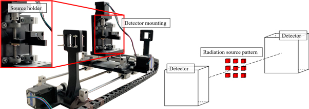
Figure 2. Experimental setup and scheme, used to generate calibration data for the timing calibration. The left picture shows the detector mountings as well as the source holder, which is connected to a translation stage system. The right picture shows the data acquisition scheme to generate calibration data for the timing calibration. The data consists of coincidences stemming from multiple source positions which are sequentially recorded. All positions are located within one plane parallel to the detector surfaces.
Download figure:
Standard image High-resolution image3. Methodology
3.1. Data acquisition
Data used for the calibration was acquired using the setup depicted in figure 2. A radiation source was placed in the source holder and coincidences were measured using a first photon trigger.
For the convex timing calibration, data stemming from one or multiple source positions within one plane in-between the detectors was sequentially collected (see figure 2). No information about the precise location of the radiation source was used. The sensor tile temperature was reported to a constant value of 0 ◦C for the semi-monolithic detector, and 2 ◦C for the one-to-one coupled detector, respectively. The excess voltage was set to 2.8 V and the validation pattern to 0 × 55:AND requiring on average 54 ± 19 optical photons.
3.2. Data pre-processing & data preparation
3.2.1. Clustering of hits
The TDCs tapped delay line (TDL) bin widths are linearly calibrated against each other assuming equally distributed trigger regarding a clock cycle (Schug D et al 2015). The measured raw data from the DPCs were corrected for saturation effects and clustered referring to one single γ-interaction (Schug D et al 2015). The cluster window was set to 40 ns, based on the distribution of all uncorrected DPC hit timestamps so that all hits can be combined into a cluster. No constraints were applied to the spatiotemporal distribution of the hits to take inter-crystal scattering into account. Furthermore, clusters showing less than 400 or more then 4000 detected optical photons were rejected to reduce noise. The uncalibrated photopeaks were located at a number of detected optical photons of about 2300 and 2800 for the slab and one-to-one coupled detector, respectively. Based on the cluster's first timestamp, a sliding coincidence window of 10 ns was applied for merging two clusters to a coincidental event, in the following called coincidence.
3.2.2. Position & energy estimation
The timing calibration utilizes information about the incident γ-interaction position inside the scintillator volume, as well as the deposited energy. The one-to-one coupled detector exploited the one-to-one design assigning the γ-interaction to the pixel registering the highest amount of photons in a cluster. The interaction position within the slab detector is estimated using gradient tree boosting (GTB) (Chen and Guestrin 2016, Müller et al 2018, 2019) models, which have been trained on calibration data acquired with an external reference provided by a fan-beam setup (Hetzel et al 2020). The scintillator was irradiated at known positions which are used during the supervised learning of GTB models. The spatial resolution (SR) representing the FWHM of the positioning error distribution is given for the one-to-one coupled detector by half of the scintillator needle pitch (2 mm), while the slab detector archived in planar and DOI positioning an SR of 2.5 mm and 3.3 mm, respectively.
The incident γ-photon's energy is calculated using a 3D-dependent energy calibration based on an averaged light pattern. Therefore, the scintillation crystal is separated into voxels, and the mean number of detected optical photons are estimated considering coincident clusters whose estimated γ-interaction-positions are within these sub-volumes (Mueller et al. 2022). The energy resolution of the one-to-one coupled detector was given to be 10.4%, while the energy resolution of the slab detector was evaluated at 11.3%.
3.3. Timing calibration
The presented timing calibration is subdivided into concatenated convex sub-calibrations, which will be referred to as stages in this work. All sub-calibrations utilize the same convex optimization problem, which is described in detail in section 3.4. The sub-calibrations can differ from another, due to different hyperparameter settings (e.g. used voxel size, used energy window, used number of radiation source positions etc), such that each stage possibly targets a different aspect of the time skews. The calibration process itself was evaluated regarding general hyperparameters of the convex calibration approach. The analysis covered the effects of different radiation source distributions, the stability of the corrections, and effects of energy restrictions in a sub-calibration. All previous finding were used for a final calibration holding multiple sub-calibrations, which was evaluated regarding their CTR performance on a semi-monolithic detector.
To draw unbiased conclusions, the acquired data was split into a calibration data set, which was purely used to find the skew corrections, and a test dataset, which was not presented during the calibration process and was solely used to evaluate the timing performance of the found correction values.
3.4. Theoretical foundation of a sub-calibration
The mathematical approach during a sub-calibration is the same for all stages and will be explained in the following. A detailed mathematical formulation can be found in the appendix.
First, both calibration detectors are subdivided into structures which can be freely chosen and represent one of many hyperparameters. At this point it is explicitly pointed out that these structures are abstract and can be represented not only by physical readout channels, but also by other objects such as, e.g. voxel volumes of the crystal or energy bins. In order to emphasize this point, these calibration structures will be called items for short. In a next step, each pair of coincident clusters (giving one coincidence) is assigned to one item on each detector. This finally allows to define sets of time differences  , corresponding to specific item combinations, e.g. for combination (k, l)

with  denoting the time difference set regarding item k on one detector and item l on the other detector, and t representing the associated timestamp. The set holds nkl
time differences. Due to the characteristics of PET, only a subset of all mathematical possible item pairs are given to be physically valid combinations representing true coincidences. To separate between valid and non-valid combinations, a threshold θ chosen by the user is set, since valid channel pairs show a significant larger amount of detected coincidences than non-valid combinations. Therefore, only those time difference sets
denoting the time difference set regarding item k on one detector and item l on the other detector, and t representing the associated timestamp. The set holds nkl
time differences. Due to the characteristics of PET, only a subset of all mathematical possible item pairs are given to be physically valid combinations representing true coincidences. To separate between valid and non-valid combinations, a threshold θ chosen by the user is set, since valid channel pairs show a significant larger amount of detected coincidences than non-valid combinations. Therefore, only those time difference sets  are further processed, whose cardinality is bigger or at least equal to this threshold

In a next step, the mean values of these time difference sets are estimated by fitting a Gaussian function to the emerging distributions using orthogonal distance regression (Boggs and Donaldson 1989). The uncertainty on the timestamp bin counts is assumed to be Possion-distributed. For the fit we considered a 1.5σ region around the peak. No background subtraction was applied. During fitting a second quality criterion is applied, namely only those combinations are further used, whose fit process showed a sum-of-square convergence. The fitted mean values  of these time difference sets, as well as the information about the item combinations are used to define a matrix equation, whose solution returns the optimal correction values to reduce the time skews. The equation in index notation is given to be

with  being the product of the matrix
M
and an item vector
being the product of the matrix
M
and an item vector  encoding in each row a different item combination. The free parameter coff accounts for a possible off-centered source position in first order approximation. For the calibration of more than two detectors, additional free parameters {coff,i} can be introduced. The optimal skew corrections
  are finally found by solving (Fong and Saunders 2012)

assuming equal weights for a equations in equation (4). Auxiliary requirements working as regularization can be encoded as additional matrix rows.
3.4.1. Effects of different geometrical source distributions
Let np be the number of included physically valid item combinations in the matrix M , such that

with na and nb denoting the number of items on detector a and b, respectively. The system of equation (5) is called overdetermined (Chan 2021), if the number of linear independent matrix rows (also referred to as rank) is bigger than the number of items used during calibration

It is guaranteed that a global optimum of equation (5) exists due to the convexity of the problem, however, it can mathematically be shown that the found minimum is unique, if the system is over- or at least well-defined

The physical equations are, per definition, mathematically independent since they are represented as single matrix rows and do not occur multiple times but only once for a given item combination (k, l) (see equation (4)). Translating this to the physical problem, a sufficient number of physical equations inside the matrix is desired to properly solve for the correction values. To increase the number of valid item combinations np
which will generate an overdeterminacy, one could use multiple (in-plane) radiation source positions. Therefore, different calibration datasets were used, each one holding coincidences from different radiation source distributions. The estimated corrections are applied to unseen data, and evaluated regarding their values with respect to the sensor geometry. In total seven datasets  evaluated, with ni
∈ {1, 3, 5, 9, 65, 225} denoting the number of radiation source positions. The spatial distribution of the source locations are depicted in figure 3. To preserve comparability between the datasets, it was ensured that each new dataset
evaluated, with ni
∈ {1, 3, 5, 9, 65, 225} denoting the number of radiation source positions. The spatial distribution of the source locations are depicted in figure 3. To preserve comparability between the datasets, it was ensured that each new dataset  holding more source positions was built by using the previous dataset
  and adding only the new data of additional source positions to it

Besides that, each pattern (except for the trivial case of n = 1) spans a square having an area of 14 mm × 14 mm, such that effects provoked by different geometrical extensions are minimized. All coincidences used for the analysis, had energy values located in a small region around the photopeak (500–520 keV). To exclude statistical effects tracing back to differences in the amount of collected coincidences, the number of collected coincidences per radiation position was kept fixed to a value of 300 000. The threshold θ was chosen such that all non-valid item combinations for the case of one radiation source are excluded (θ1 = 200), and then linearly scaled corresponding to the amount of source positions,

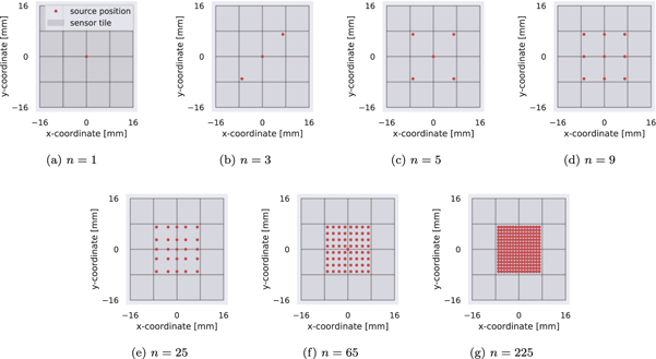
Figure 3. The pattern of the used radiation source positions. The sensor tile is depicted as gray background and separated regarding the 4 × 4 DPCs. Except for the case of three source positions, which shows a 2-fold rotational symmetry, all other distributions have a 4-fold rotational symmetry. All patterns, except for n = 1 and n = 3 cover the same detector area comprising 14 mm × 14 mm.
Download figure:
Standard image High-resolution image3.4.2. Stability of the estimated corrections
Assuming a stable behavior of the estimated corrections, one would expect that the corrections converge to zero after a desirable low number N of repetitions

with  denoting the correction of item i in repetition n.
To evaluate a measure of stability of the estimations, the calibration process was repeated and applied several times subsequently. This process was performed for the case that no regularization terms are included, and for the case that regularizations are utilized. In the latter case two additional terms are included in the matrix, one for each detector, namely the corrections of all abstract channels of the corresponding detector have to add up to zero. The study was conducted using the pattern depicted in figure 4 comprising 81 source positions with a pitch of 3 mm.

Figure 4. Pattern comprising 81 different source position covering an area of 24 mm × 24 mm, with a pitch of 3 mm. This radiation pattern was used for the analysis of the correction stability, the effects of energy restrictions, and for finding corrections for the CTR evaluation.
Download figure:
Standard image High-resolution image3.4.3. Influence of energy restrictions & statistics
The calibration was based on five different energy windows ([300, 700] keV, [350, 650] keV, [400, 600] keV, [411, 561] keV, and [500, 520] keV) and subsequently applied to unseen evaluation data to evaluate how the energy window of the calibration data affects the quality of the estimated corrections. Minding, that a broader energy window implies a larger number of coincidences, the number of coincidences are fixed to 10 00 000 for each window to exclude statistical effects. The same calibration data as in section 3.4.2 was used, comprising 81 source positions with a pitch of 3 mm(see figure 4). To study statistical effects of the calibration, the previous analysis was repeated without limiting the amount of calibration data to a fixed number. By doing so, the calibration based on a larger energy window comprised much more data resulting a better statistics.
3.4.4. CTR evaluation
For a CTR evaluation, all previous findings were used within an calibration of a setup with a one-to-one coupled and a semi-monolithic detector. The calibration holds six sub-calibrations, where in two stages the calibration items were represented by hardware components, namely TDC-regions and readout-channels, and the other four stages were based on sub-volumes of the scintillation crystals with different size. The first two voxel stages, were based on voxels using no DOI-information, the voxel's base area was given by the TDC- and readout-regions, respectively. The third voxel stage covered only DOI information, no planar information was used. The last stage used the full 3D information, namely planar and DOI information.
The first two stages tried to target electrical time skews, while the following stages addressed crystal-related skews. No time walk effects were included in this analyzed. The calibration dataset was based on an energy range of 350–650 keV comprising 9 × 9 radiation positions with a pitch of 3 mm (see figure 4). For comparison, a similar calibration was also applied to a setup using the same sensor technology but two one-to-one coupled detectors. The CTR for a pure slab setup was extrapolated using equation (21) shown in the appendix. The CTRs were estimated by numerically determining the FWHM. The evaluation was performed for two different energy windows (300–700 keV and 411–561 keV) and an optional filter ensuring that the main pixel and the first timestamp was provided by the main DPC, and a full pixel row (covered by a slab) was read out.
4. Results
4.1. Effects of different geometrical source distributions
As it can be seen in figure 5, all analyzed equation systems are well- or overdetermined. By increasing the number of used radiation positions, the rank of the matrix also increases, while at some point the curve starts to converge against a stable value. However, after a certain point is reached, there is a slight decrease visible. This behavior can also be confirmed by the detailed analysis visible in figure 7, where the number of physical equations per calibration structure of detector a is depicted, with the additional information regarding the spatial distribution of the channels. Central structures (see figure 6) reach the maximal number of possible equations that can be used for the equation system (see figure 7), while side- or corner-located structures show a lower number of physical equations.
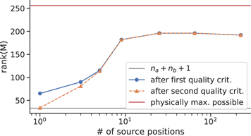
Figure 5. Progression of rank(M) in dependence of the number of used radiation source positions. The physical maximal possible number of item combinations encoded as linear independent matrix rows is given by all combination of detector a and b to be equal to 16 × 16. The first and second quality criterion is given by exceeding a given threshold θ and ensuring the convergence regarding the sum-of-squares of the fit.
Download figure:
Standard image High-resolution image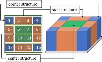
Figure 6. Two examples of different geometrical classes of calibration structures. The left image shows an example where the items are represented by TDC regions. The right image shows a possible configuration of calibration items represented by volumes of the scintillation crystal. For the further evaluations regarding characteristics of a convex model, the item configuration of the left picture is used.
Download figure:
Standard image High-resolution image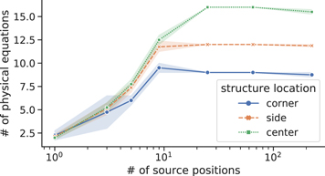
Figure 7. Number of physical equations per channel region depicted for detector a in relation to the used number of radiation source positions.Since detector b comprises 16 items within this stage, each channel of detector a could form up to 16 pairs with items from detector b. The colored area represents a 1 sd-band around the calculated marked mean values.
Download figure:
Standard image High-resolution imageFigure 8 shows the estimated corrections for each channel related to the used number of radiation source positions. One can clearly see, that for most of the items, the estimated corrections obtained with only one source position differ strongly from the other estimated corrections. In the majority of the cases, the estimated corrections of calibrations using 25 or more radiation positions are close together, whether the other calibrations differ in their estimations. Furthermore, some calibration items show in general a large spread regarding the corrections (e.g. b13), while the estimations for other items (e.g a6) are very similar.

Figure 8. Estimated time skew corrections in relation to the used number of radiation source positions. The concrete values regarding the different numbers of source positions are marked as colored dots. To better relate the values, a boxplot (black and gray lines) of the underlying points is also shown behind. Since the different calibration datasets comprise the same measurement run, the estimated correction should be the same regardless of number of radiation source positions. As it can be seen, the estimated corrections obtained with the dataset comprising only one source differ strongly from the others.
Download figure:
Standard image High-resolution image4.2. Stability of the estimated corrections
By using the naive approach without any regularization terms, the corrections of both detectors converged already after the first iteration against constant values unequal to zero, which themselves converged to zero with increasing number of iterations (see figure 9(a)). As it can be seen in figure 9(b), by introducing the additional regularization terms to the matrix, the corrections converge directly to zero and stay there for at least ten iterations.
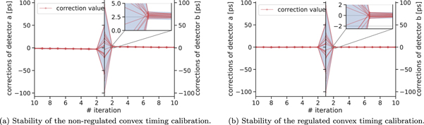
Figure 9. Stability of the estimated corrections for both detectors. For the non-regulated calibration, the corrections converge to not directly to zero (see the zoom-in plot in the upper right corner).
Download figure:
Standard image High-resolution image4.3. Influence of energy restrictions & statistics
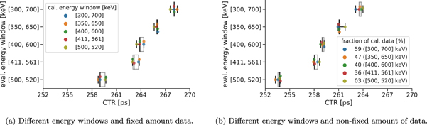
As one can see in figure 10(a), in the majority of evaluations, the corrections obtained with calibration data based an narrow energy window of 500–520 keV results in the best CTRs. On the other hand, there's no energy window which is clearly connected to the worst performing corrections.
Figure 10. Obtained CTRs after correction of an unseen evaluation dataset with respect to different energy windows with fixed or non-fixed amount of calibration data. The concrete values regarding the different energy windows or fractions of calibration data are marked as colored dots. To better relate the values, a boxplot (black and gray lines) of the underlying points is also shown behind.
Download figure:
Standard image High-resolution image
Regarding statistical effects (see table 1) on the convex optimization figure 10(b) reveals that the calibration based on the statistically least significant dataset (500–520 keV) provides corrections resulting in four of the five evaluations the worst CTRs compared to the different calibrations. The estimated corrections from the calibration based on the largest energy window worked best for evaluations associated to large energy windows (300–700 keV and 350–650 keV), while the calibration based on data from 350 to 650 keV worked best for test data from 411 to 561 keV and 500 to 520 keV. In general, one observes that the CTRs achieved in figure 10(b) are smaller compared to those in figure 10(a).
Table 1. Statistical significance of the calibration data regarding different energy windows, if the number of coincidences is not restricted to a fixed number. The relative number of coincidences* is connected to the available coincidences if no restrictions regarding the energy window are applied (n = 304 98 923).
| Energy window [keV] | Total no. of coinc. | Rel. no. of coinc.* [%]) |
|---|---|---|
| [300, 700] | 18 142 527 | 59 |
| [350, 650] | 14 403 316 | 47 |
| [400, 600] | 12 180 456 | 40 |
| [411, 561] | 11 007 180 | 36 |
| [500, 520] | 1 001 083 | 3 |
4.4. CTR evaluation
The obtained CTR values based combination of slab and one-to-one coupled detector are listed in table 2 under the column SD-OD. The timing performance of two one-to-one coupled detectors is listed under the column denoted as OD-OD. The CTR of a pure slab setup is given under SD-SD*, and was, for practical reasons, extrapolated using equation (21) (Borghi et al 2016). Filter F ensures that the main pixel and the first timestamp is provided by the main DPC, and a full pixel row (covered by a slab) is read out.
Table 2. Performance of the timing calibration scheme. The slab detector is abbreviated as SD, while OD represents the one-to-one coupled detector. The Filter F ensures that the main pixel and the first timestamp is provided by the main DPC, and a full pixel row (covered by a slab) is read out. Columns marked with * have been determined by extrapolation using equation (21) (Borghi et al 2016). The uncertainties on the reported CTRs are in the order of 0.1 ps and, therefore, concerning the reported values neglectable.
| Filter | CTR [ps] | ||
|---|---|---|---|
| SD-OD | OD-OD | SD-SD* | |
| E ∈ [300, 700]keV | 237 | 234 | 240 |
| E ∈ [411, 561]keV | 231 | 228 | 234 |
| E ∈ [411, 561]keV ∧ F | 223 | 224 | 222 |
5. Discussion
The results show, that the calibration concept generally works and that attractive CTRs down to 240 ps for a broad energy window of 300–700 keV can be achieved using a first photon trigger and a tile temperature of approximately 0 ◦C. Although this temperature setting is challenging on the system level, it can be realized using liquid cooling systems, as demonstrated for the application in PET/MRI (Mueller et al 2019). It can be expected that for increasing SiPM temperatures, the detectors' dark count rate also increases. In conclusion, this results in increased dead-time due to a surplus of non-validated triggers. The DPC trigger scheme should be set to a higher level to prevent the loss of detector sensitivity. However, this higher number of required optical photons, typically deteriorates the timing resolution (Schug et al 2017). All tested hyperparameters show a strong influence on the timing calibration.
The effect, that rank( M ) decreases for the case of 225 radiation positions (see figures 5 and 7) might be reasoned by the different pitches regarding the radiation source grid and also by a non-optimized usage of the threshold θ (see equation (10)). Whereas for the case of 65 source positions, the pitch is given to be 2 mm, in the case of 225 positions the pitch equals 1 mm, which is smaller than the spatial resolution of the detector. Minding this, there could be a deterioration regarding the items assignment, such that a linear scaling of the threshold θ (see equation (10)) might not be suitable for very small position pitches.
Since the calibration data was acquired within the same measurement run, it can be assumed that the time skews with respect to different calibration datasets should always be the same. The analysis reveals that there are strong differences (see figure 8) in the estimated skew values, especially for the case where data from only one radiation source position is used. This observation indicates, that the estimations differ in their quality and that calibrations based on a large number of source positions (e.g. 25 or more) are more capable of finding the more generalized skews compared to calibrations using less positions. However, care should be taken regarding the pitch of the grid positions. It seems to be optimal to use many radiation sources covering a maxed out area of the detector, such that the pitch is bigger than the detector's spatial resolution while the rank of the matrix is increased. Section 4.2 reveals that for both kinds of calibration (regularized & non-regularized) the estimated corrections converge to zero and show sufficient stability. Contrary to the regularized case, for the non-regularized calibration the estimations converge not directly to zero, but to a value Θa,b ≠ 0. This behavior is harmless for the case that the corrections {si,1} of the first iteration are sufficient big, such that

However, for the case that the corrections are in the same order of magnitude, such that

the algorithm might deteriorate and converge to arbitrary high values to satisfy equation (5), and in the end not representing the physical system. To avoid these phenomena, regularization terms should be included in the matrix since they provoke a convergence to zero as can be seen in figure 9(b).
The analysis of section 4.3 regarding the energy restrictions and statistics showed that not only photopeak events are necessarily needed for the calibration, but a sufficiently good statistic has to be evaluated with higher priority. Given the same statistics, the calibration model of a narrow photopeak data set gives better results. This observation could indicate that the determination of the mean of the time differences is favored by sufficiently good statistics. However, in a calibration data set with a very wide energy window, additional effects besides the time skews can play a role, e.g. time walk, which in turn bring additional uncertainty to the determination of the time skew corrections and was not considered in this calibration.
The obtained CTR values of the final calibration scheme show, on the one hand, that the presented timing calibration is strongly capable of reducing time skew effects, and on the other hand, they underline on the bench top level that slabs are on a good way to become a promising alternative to clinical used segmented detectors. The obtained CTR of a pure semi-monolithic and a pure one-to-one coupled setup differ in the maximum only about 3% (6 ps).
6. Conclusion
The presented work reveals the capability of the presented bench top timing calibration. The presented calibration approach was evaluated by using detectors utilizing digital SiPMs. However, it can be expected that the shown calibration technique will also work for analog SiPMs, due to the general formalism of using calibration items. The work shows, that the quality of the corrections themselves is positively effected by incorporating multiple in-plane radiation source positions which substantially increase the overdeterminacy of the convex optimization problem. Besides this, two major component of the calibration are the underlying statistical significance of the calibration dataset, as well as the coincidences' energy range. The results indicate, that a sufficient statistic should be ranked higher in importance compared to including only events of a narrow energy window around to 511 keV peak. For future research, we want to improve the calibration formalism and approach in terms of calibration time and the needed number of source positions so that it also becomes well-applicable for full-scale PET scanners to improve the timing performance on the system level. In a complete scanner, an arrangement of multiple point sources, line sources or a dedicated phantom may be used to mimic the various source positions. In this case, the positioning capabilities of the employed detectors can be utilized the select corresponding LORs in the scanner volume. The concrete implementation is open for future work.
Acknowledgment
This work was funded by the German Federal Ministry of Education and Research under contract number 13GW0621B within the funding program 'Recognizing and Treating Psychological and Neurological Illnesses - Potentials of Medical Technology for a Higher Quality of Life' ('Psychische und neurologische Erkrankungen erkennen und behandeln - Potenziale der Medizintechnik für eine höhere Lebensqualität nutzen').
: Appendix. Mathematical formulation of the analytical timing calibration
The calibration procedure is mathematically based on setting up a matrix equation containing information from time difference relations between two facing detectors, called a and b. Each of the detectors is separated into calibration structures, also called items, resulting in na items for the case of detector a, and nb items for the case of detector b. An item represents an abstract object, with the requirement that coincident cluster or at least their corresponding timestamps can be assigned uniquely to one item on a and one on b.
Formally two functions ϕa
, ϕb
are defined, which map each coincidence i consisting of two coincident clusters timestamps to one a-item and one b-item, where the set of items of a and b are denoted as  and
and  respectively

A selected timestamp of detector x ∈ {a, b} that belongs to coincidence i and has been assigned to item cz
will be denoted as tz,i
. The detector index x can be suppressed since the timestamp's detector identification is given by the item address z. In the next step, one looks at the timestamp differences of item pairs (k,l), where item  and item
  such that a new set
  can be defined

with nkl
representing the number of coincidences that are assigned on a to item ck
and on b to item cl
. Before setting up the matrix equation, one iterates over all possible item pairs (k,l) and estimates the mean time difference  by fitting a Gaussian function to the distribution of
  . At this point, one has to compress the information about the item combinations and their corresponding mean time difference into a suitable form, such that it is possible perform an optimization regarding time skews of the items. Therefore, one aims to mimic equations like

where coff is seen as a free parameter. An item vector  is formed, holding all the calibration items, as well as the additional parameter coff,

Mathematically, the inclusion of only one free-parameter can be seen as a first-order approximation since in the most-general way one could also introduce a new vector  giving additional free parameter for each channel. Besides that, also a mean-time-difference-vector

containing time difference relations regarding different item combinations can be defined. The rows of matrix
M
are filled with −1, 0 and 1, based on the item vector  and the item pairs associated with the corresponding entries of
  . Besides that, regularization terms in form of new rows can be included in the matrix, such that it is ensured that the corrections can not converge to arbitrarily high values. The resulting equation system consisting of
M
,
. Besides that, regularization terms in form of new rows can be included in the matrix, such that it is ensured that the corrections can not converge to arbitrarily high values. The resulting equation system consisting of
M
,  , and
, and  is given by

The corrections for each item, contained in  , are subsequently found by minimizing a loss function with respect to
  , e.g. minimizing the Euclidean norm

The CTR of a pure detector system α α holding the same type of scintillation detectors (α) can be extrapolated using the time resolution of a mixed system α β and the corresponding other pure system β β (Borghi et al 2016)
