


ABSTRACT
Solar wind plasma and compositional properties reflect the physical properties of the corona and its evolution over time. Studies comparing the previous solar minimum with the most recent, unusual solar minimum indicate that significant environmental changes are occurring globally on the Sun. For example, the magnetic field decreased 30% between the last two solar minima, and the ionic charge states of O have been reported to change toward lower values in the fast wind. In this work, we systematically and comprehensively analyze the compositional changes of the solar wind during cycle 23 from 2000 to 2010 while the Sun moved from solar maximum to solar minimum. We find a systematic change of C, O, Si, and Fe ionic charge states toward lower ionization distributions. We also discuss long-term changes in elemental abundances and show that there is a ∼50% decrease of heavy ion abundances (He, C, O, Si, and Fe) relative to H as the Sun went from solar maximum to solar minimum. During this time, the relative abundances in the slow wind remain organized by their first ionization potential. We discuss these results and their implications for models of the evolution of the solar atmosphere, and for the identification of the fast and slow wind themselves.
Export citation and abstract BibTeX RIS
1. INTRODUCTION
The Sun is a variable star that changes on multiple spatial and temporal scales. The most apparent cycle has a period of approximately 11 years and involves significant changes to both the magnetic structure and the radiative and particle emission from the solar corona. The Sun's evolution over this cycle is obvious to the remote observer and includes well known variations in the number and distribution of sunspots and active regions as well as variation in the number of flares and coronal mass ejections (CMEs; e.g., Gopalswamy et al. 2003). These measures of solar activity reflect the underlying physical driver of these changes—the solar dynamo and thus the magnetic field of the solar corona, where the solar wind originates. The physical properties of the source regions lead to two quasi-stationary types of solar wind streams that can be observed near the ecliptic: a steady, faster solar wind originating from polar coronal holes and particularly equatorial extensions of coronal holes to low latitudes, and a slower, more variable wind that is found near the heliospheric current sheet (HCS), where the magnetic polarity changes (see Zurbuchen 2007 and references therein). Near solar minimum, the slow solar wind is confined within 20° of the relatively flat HCS. Away from solar minimum, the structure of the wind becomes more complex and the slow wind fills a much larger portion of the heliosphere, extending up to 45° from the HCS (Zhao et al. 2009). At elevated solar activity levels, transient flows of plasmas—such as from CMEs—contribute an increasing percentage of solar wind plasma, perhaps contributing in excess of 15% of all heliospheric plasmas (Webb & Howard 1994, and references therein).
Since its launch in late 1997, the Advanced Composition Explorer (ACE; Stone et al. 1998) and especially its Solar Wind Ion Composition Spectrometer (SWICS; Gloeckler et al. 1998) have provided an unprecedented look at this evolution of the solar wind and also the inner state of the solar wind. Of particular interest are changes in the properties of the heavy ions, which reflect the evolution of the properties of coronal sources of the solar wind during the activity cycle. By investigating the long-term evolution of the solar wind composition, we seek to learn about global changes in the ambient solar atmosphere and in the acceleration and heating mechanisms.
A recent analysis by von Steiger & Zurbuchen (2011) focused on high-latitude coronal holes has shown an overall decrease in the charge state composition of C, O, Si, and Fe since the minimum of solar cycle 22. This decrease was consistent with a 10% reduction of electron temperature in coronal holes during polar passes of the nearly 20 years of the Ulysses mission, if ionization equilibrium is assumed. However, through a detailed analysis of the elemental abundances, von Steiger & Zurbuchen (2011) found a rather robust and persistent distribution (within the uncertainties) of heavy elements relative to the abundance of oxygen, consistent with the results of von Steiger et al. (2000).
A comparable analysis has been performed neither for slow wind nor for the fast wind observed around the ecliptic plane. The goal of the present work is to study the solar cycle evolution of both the fast and slow solar wind as seen by ACE in the ecliptic plane; in particular, we focus on both ionic charge states and elemental abundances of the heavy elements.
We consider the ACE data measured by SWICS from 2000 to 2010, using the most extensive in situ heavy ion data set to date and made publicly available by the ACE team. We focus on two key questions concerning the evolution during 2000–2010 that will be addressed in the subsequent sections:
- 1.How do the solar wind plasma parameters, charge state distributions, and element composition evolve with the solar cycle?
- 2.Do the fast and slow wind properties evolve in the same way?
We will discuss these questions in the context of theories for the solar wind origin and acceleration of the solar wind. Section 2 presents a brief overview of the fast and slow solar wind properties, and Section 3 describes the observations we use in this work. The basic distribution of the wind parameters is discussed in Section 4, while in Sections 5 and 6 we discuss the time evolution of the fast and slow wind properties. Section 7 summarizes the results.
2. SOLAR WIND ELEMENTAL AND IONIC COMPOSITION
Heavy ion composition is determined low in the corona where the solar wind is accelerated (Owocki et al. 1983, and references therein) and reflects the local electron temperature and density history of the wind ions before they freeze-in (Hundhausen et al. 1972). Once the ion composition is set in the low corona (within ∼4 Rs), it will not change as it propagates far out into the heliosphere (Hundhausen et al. 1968). For this reason, heavy ion composition is a vital tool for tracing plasma parcels back to the corona and for understanding the physical processes that are at work in solar wind acceleration regions.
The charge states of  and
and  have long been used to differentiate source regions of the solar wind in the innermost solar corona (e.g., Zurbuchen et al. 2002; Zhao et al. 2009). Recently, Landi et al. (2012a) showed that C6 +/C4 + was actually a more sensitive indicator of electron temperatures in the corona and therefore an even better indicator of solar wind type and region of origin. Contrary to the charge state ratios of O and C, the average charge state of Fe (QFe) has been shown to be a sensitive tracer of electron temperatures at larger heights, up to 4 Rs, so that it can be used as a measure of the evolutionary properties in the far corona (e.g., Lepri et al. 2001; Lepri & Zurbuchen 2004; Gruesbeck et al. 2011).
Solar wind plasma also provides a sample of the element composition of the source regions on the Sun. Solar wind abundances are often well organized by first ionization potential (FIP) in a very similar way as in the inner corona (Geiss 1982; Zurbuchen et al. 1998), so that the source region of the wind must be located at chromospheric or low corona heights. There is evidence that gravitational settling, waves, and mass- and charge-dependent acceleration mechanisms further modify this elemental abundance as it is expelled out of the corona into the solar wind. Elemental abundances therefore provide unique tools to trace the solar wind to its solar source.
This paper is focused on the large-scale evolution of the near-ecliptic heliosphere during the transition from solar maximum through the deepest solar minimum since the space age (e.g., Mewaldt et al. 2010; Russell et al. 2010). Due to the latitudinal expansion of the solar wind, the near-ecliptic plasmas can originate from a wide range of latitudes in the Sun from near the solar equator to as high as 40°–50°. In that sense, the decade-long ACE observations are likely to reflect the evolution of the global solar corona. This evolutionary transition is shown in Figure 1(a), which shows the logarithmic density (or frequency) of observations of solar wind proton velocity during every Carrington rotation from 2000 to 2010.5. Also shown in Figure 1(b) are the two measures of solar activity—the sunspot number (SIDC Team 2000–2010) and the number of interplanetary coronal mass ejections (ICMEs) (multiplied by 10) observed (Richardson & Cane 2010) in each Carrington rotation.
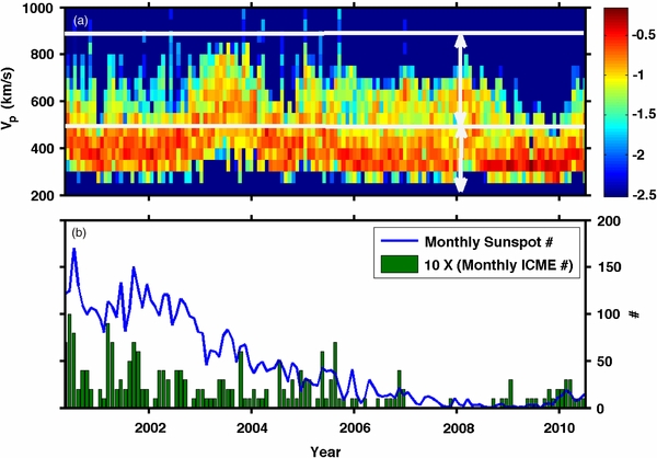
Figure 1. (a) Logarithmic density (or frequency) of observations of solar wind proton velocity during every Carrington rotation from 2000–2010.5. Solid horizontal lines mark the solar wind type boundaries between fast (500–900 km s−1) and slow solar wind (200–500 km s−1). (b) Two measures of solar activity—the sunspot number (SIDC Team) and the number of ICMEs (multiplied by 10) observed (Richardson & Cane 2010) in each Carrington rotation.
Download figure:
Standard image High-resolution imageFigure 1(a) clearly demonstrates the dominance of low-speed solar wind (V < 500 km) during most of the duration of the declining phase of solar cycle 23. Speeds are plotted as low as 250 km s−1, but seem to peak around 400 km s−1, consistent with observations by Helios (Schwenn 1990) and others.
Using multi-point inner heliosphere observations, Schwenn (1990) demonstrated that quasi-stationary solar wind in the heliosphere is largely a two-state phenomenon much closer to the Sun, but that the velocity gradients flatten due to fluid interactions between fast, coronal-hole-associated wind and the streamer-associated slow wind. That flattening is clearly seen in many of the Carrington rotations: rather than providing a second maximum, consistent with high-latitude observations and also inner heliosphere observations, the fast wind only provides an extension to high velocities to a distribution that peaks around 400 km s−1. There are exceptions to this, such as in late 2007, where the two sources can be easily discerned—a distribution peaking around 400 km s−1 and one peaking around 600 km s−1. The time period in 2003–2004 deserves special attention because of its comparatively high average due to low-latitudes coronal holes and also high-velocity transients.
Figure 1(a) also includes all transients such as ICME-associated plasmas. Typically, they can be discerned in this plot through high-velocity extensions during individual Carrington distributions. When there are many ICMEs, as shown in Figure 1(b), many such extensions are observed in Figure 1(a), and the extensions are rare during solar minimum where ICMEs are a much rarer occurrence.
One of the criteria most used to identify the solar wind type are its compositional features. For example, coronal-hole-associated fast wind is characterized by lower ratios of O7 +/O6 + and C6 +/C5 + as well as slightly lower charge states of Fe than in the slow solar wind (e.g., Von Steiger et al. 2000; Zurbuchen et al. 2002; Zhao et al. 2009), indicating that the two wind types experience a very different history before freeze-in and therefore escape from very different source regions. Also, the fast solar wind is characterized by abundances of elements with FIPs lower than 10 eV that are similar to those measured in the photosphere, while the slow solar wind is enhanced in ions of elements with FIP < 10 eV compared to the photosphere (Von Steiger et al. 2000), indicating that the source of the slow wind is most similar to large coronal loops (Raymond et al. 1997; Feldman et al. 1999, 2005; Raymond 1999; Fisk 2003).
It has been shown by Gloeckler et al. (2003) that there is an overall correlation between ionic charge states and velocity of quasi-stationary solar wind streams. Even though ionic charge states do not undergo dynamic evolution beyond their freeze-in point, they nonetheless carry an overall velocity signature. The exact reason for this correlation is not clear. It can be argued that this relates to the velocity-dependent freeze-in process (Buergi & Geiss 1986; Ko et al. 1997; Zurbuchen et al. 2012), which would tend to lead to a freeze-in location closer to the Sun in faster wind. Such an interpretation would lead to profound consequences about the temperature, density, and velocity profile of a plasma parcel during its heliospheric expansion, and can be used to empirically determine those profiles as shown by Landi et al. (2012b). On the other hand, this correlation has been interpreted to be a signature of solar wind sources and energization near the corona (Fisk et al. 1999; Schwadron & McComas 2003). In any case, it might be expected that ionic charge states are affected by the long-term evolution of the solar wind velocity, density, and temperature due to the solar cycle.
3. OBSERVATIONS
Measurements of heavy ion charge state and elemental composition are obtained from SWICS on board ACE. ACE was launched in 1997 and currently sits upstream of the Earth at the L1 point, continuously immersed in the solar wind. ACE/SWICS currently measures the solar wind composition and has since early 1998.
The SWICS main channel is a time-of-flight (TOF) mass spectrometer paired with energy-resolving solid-state detectors (SSDs) and an electrostatic analyzer (ESA; Gloeckler et al. 1998). The ESA allows only ions within the given energy per charge E/Q passband to enter the TOF section of the instrument. After passing through the post-acceleration region (which supplies an additional ∼25 keV/e for each ion), the ion enters the TOF telescope by passing through a carbon foil and releasing secondary electrons that initiate a start timing signal at the start MCP. At the other end of the TOF telescope, the electrons impact the SSD, releasing secondary electrons, which then produce a stop timing signal at the stop MCP. These start/stop MCP signal pairs yield a measurement of an ion's TOF, which can then be used to calculate the ion speed. The E/Q, TOF, along with the residual energy measured by the SSDs enable particle identification. These measurements allow the independent determination of mass, M, charge, Q, and energy, E, and are virtually free of background contamination. These triple-coincidence measurements allow nearly unambiguous identification of a wide range of charge states of He, C, O, Fe, etc., in the energy per charge range of 0.49–60 keV/e, which covers the thermal solar wind energies.
SWICS auxiliary channel pairs an ESA with an SSD and is optimized to measure H+ and He2 +. The auxiliary channel is parallel with the main channel and shares the same ESA and post-acceleration. Analysis of the E/Q spectra allows calculation of H+ and He2 + density, velocity, and thermal velocity. In this paper, we only use the measurements for H+ from this channel as the main channel provides more robust measurements of He2 +.
These measurements enable calculation of the densities of heavy ions. These densities can then be used to calculate charge state distributions of C, O, Si, and Fe and other ions. In addition, ion densities can also be used to calculate the elemental abundance ratios relative to O or H. The data have to be corrected for instrument efficiencies, measurement duty cycle, and event priorities that affect the probability of these ion measurements to be transmitted to the ground (von Steiger et al. 2000; Lepri et al. 2001).
Because of the long duration of the measurement, long-term efficiency changes of the SWICS instrument can be an issue—however, we can safely exclude an instrumental cause based on the analysis performed in the Appendix of von Steiger & Zurbuchen (2011), whose conclusions were confirmed through thorough trend analysis of the SWICS data. We refer to this Appendix for further instrumental details and also descriptions of the analysis procedure used here.
4. THE LOGNORMAL NATURE OF SOLAR WIND PARAMETERS
In order for us to adequately describe the long-term behavior of solar wind plasma and compositional quantities, it is important to understand the nature of the stochastic distribution of the relevant quantities. For example, if distributions are non-Gaussian, averages have different meanings than with Gaussian statistics.
Burlaga & Lazarus (2000, and references therein) reported that the statistical variations in the bulk solar wind parameters of Np, Vp, Tp, and B behave according to a lognormal distribution. They describe the fluctuations as "... highly variable, episodic, intermittent, and non-uniform..." (p. 2357). These non-Gaussian distributions of plasma parameters of the solar wind are an important signature of the very nature of turbulence and the sources of the solar wind (see, i.e, Marsch & Tu 1997, or Pagel & Balogh 2003). Generally, quantities with lognormal distributions can be interpreted as multiplicative products of many independently random variables.
The stochastic behavior of solar wind compositional quantities has been reviewed by Bochsler (2000). Also, a recent study of O/H by von Steiger et al. (2010) found that the prevalent distributions are lognormal in nature. Generally, we find that both ion charge state ratios and elemental composition ratios exhibit non-Gaussian properties well approximated by lognormal characteristics. Figure 2 shows sample distributions for O7 +/O6 +, C6 +/C4 +, O/H, and C/H in solar wind slower than 500 km s−1 taken during solar maximum (2000–2002). Periods of transients, such as ICMEs, were excluded based on the list by Richardson & Cane (2010). We have superimposed Gaussian fits (blue lines) to the logarithm of the number of occurrences in each bin to verify the lognormal nature of these distributions. With the only exception of C/H, which shows an asymmetric tail toward lower values, the fitted curves reproduce the observed distributions very closely. The lognormal nature of the plasma parameter distributions allows us to calculate means in lognormal space rather than in the linear space, and use the standard deviation of those means to create upper and lower bounds for variability of the data, thus ensuring that 68% of our data lies within the limits we provide.
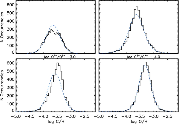
Figure 2. Sample distributions for the logarithm of the ratios of O7+/O6+ (shifted by −3 to fit on the same scale as C/H), C6+/C4+ (shifted by −4 to fit on the same scale as O/H), C/H, and O/H in solar wind slower than 500 km s−1 taken during solar maximum (2000–2002). Periods of transients, such as ICMEs, were excluded based on the list by Richardson & Cane (2010). Gaussian fits (blue lines) to the logarithm of the number of occurrences in each bin are shown to verify the lognormal nature of these distributions.
Download figure:
Standard image High-resolution image5. LONG-TERM BEHAVIOR OF HEAVY IONS AT ACE
Since wind speed is traditionally one of the parameters used to discriminate between fast and slow solar wind, we separate our solar wind in two bins shown by the solid horizontal lines in Figure 1, with the slow wind ranging from 200 to 500 km s−1 and the fast wind ranging from 500 to 900 km s−1. We set our fast wind threshold at >500 km s−1, 100 km s−1 lower than the threshold of >600 km s−1 by Schwenn (1990), based on the distributions of speeds shown in Figure 1(a), which falls off abruptly during solar minimum above 600 km s−1, when we are most interested in the behavior of the fast wind. Should we have set our limit at >600 km s−1 the trends would be preserved, however, the measurements become spottier where there are few data points with Vp > 600 km s−1. Here, we focus on averages of all wind properties over the length of a Carrington rotation in each of these two velocity bins and have found the results to be robust within the statistical limits of the data.
Figures 3 and 4 show the original data taken during two Carrington rotations, one at solar maximum and one at solar minimum. Figure 3 shows key solar wind plasma and composition data for CR 1987 measured during solar maximum in 2002 with a one-hour time resolution for the plasma data and two-hour time resolution for the composition data. The top four panels show the solar wind proton speed, kinetic temperature, and density, measured from the SWEPAM instrument on board ACE, as well as magnetic field magnitude and the field longitude and latitude (λ (blue) and δ (red), respectively) from MAG, also on ACE. Further, we show charge distributions of Fe, O, and C as well as the Fe/O element abundance ratio. This Carrington rotation period includes both fast and slow wind as well as a few ICME transients, whose beginning and end are marked by the full and dashed vertical red lines, respectively. These ICME transients, identified by Richardson & Cane (2010), are excluded from this analysis because they are known to have significantly different compositional properties (Zurbuchen & Richardson 2006 and references therein).
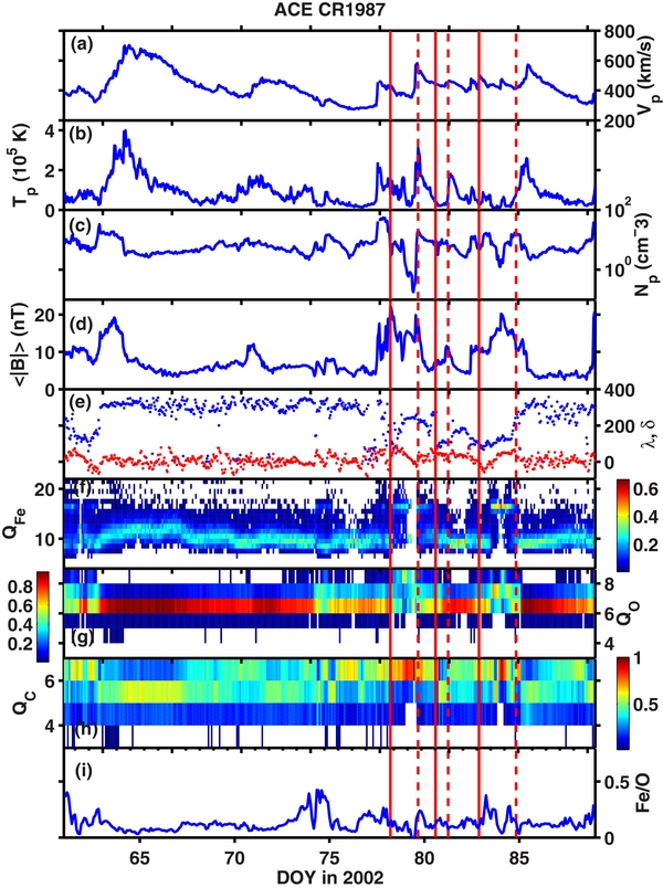
Figure 3. Key solar wind plasma and composition data for CR 1987, during solar maximum, from ACE are plotted. The panels show (a) solar wind proton speed (Vp), (b) proton kinetic temperature (Tp), (c) density (Np), (d) magnetic field magnitude 〈|B|〉, (e) magnetic field latitude (δ (red)) and longitude direction (λ (blue)), (f)–(h) charge distributions of Fe, O, and C as well as (i) Fe/O element abundance ratio. This Carrington rotation period includes both fast and slow wind as well as a few ICME transients, whose beginning and end are marked by the full and dashed vertical red lines, respectively.
Download figure:
Standard image High-resolution image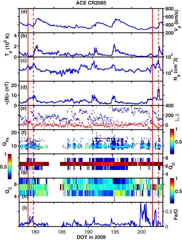
Figure 4. Same as Figure 3 but for CR 2085 during solar minimum.
Download figure:
Standard image High-resolution imageFast solar wind streams can be identified during time periods of high speed and enhanced proton kinetic temperature. Compositionally, coronal-hole-associated wind is indicated by comparatively lower ionic charge states, especially in C and O, as well as lower Fe/O values. Slow, streamer-associated wind is much more variable; its most obvious signatures are its higher ionic composition and larger Fe/O ratio (Zurbuchen 2007 and references therein).
Figure 4 shows data in the identical format but for CR 2085 which occurred in 2009 during the deepest solar minimum since the beginning of in situ observations from space. Again, both wind types are visible and indicated during this CR, although their relative contributions shifted. While we only had two clear passages through the HCS during CR 1987, the structure at minimum is more complicated, presumably because the HCS, although closer to the ecliptic, is warped, leading to multiple passages and also a tendency to measure predominantly slow, streamer-associated solar wind. But, even in this situation, fast, coronal-hole-associated wind is present, allowing for a comparison of all wind types from solar minimum to maximum.
There are significant differences between CR 1987 and CR 2085 that we will show to be part of general trend that occurs within the ten-year period studied here. For example, the proton temperatures, density, and magnetic field flux density are significantly lower in CR 2085 as compared to CR 1987. However, the most significant change consists of a large drop in all abundances of the heavy ions as evidenced by the spottiness of the ion composition measurement due to lower densities throughout and is also evident in the Fe/O panel. Additionally, there is a qualitative change in charge state distributions which are much narrower near solar minimum and shifted toward lower charge states. This is particularly obvious when comparing distributions of O and C in the bottom two panels between Figures 3 and 4. This shift to lower ionic charge states has already been observed in coronal-hole-associated fast wind at high ecliptic latitudes, but is evidenced here also for slow wind. The transition to lower densities of heavy ions has not been described previously.
We now examine the long-term behavior of the bulk solar wind along with heavy ion charge state indicators including select ions ratios and the average Fe charge state from ACE SWICS, as depicted in Figures 5 and 6. We separate slow solar wind from the fast solar wind, based on solar speed, as defined in Figure 1(a), and calculate Carrington rotation averages of plasma data (one-hour time resolution) and composition data (two-hour time resolution), excluding all missing data for all parameters, to look for the behavior within different solar wind types. Typically, we have less than 5% of missing data, depending on the actual quantity, with sufficient amounts of data to generate good averages. This specific separation based on speed has been used in order to eliminate compositional selection biases into an analysis of compositional trends. We have used a variety of speed cutoffs and other selection criteria, and have found the results that will be discussed below to be robust and relatively independent of the actual criterion. ICME periods (as identified by R&C) have been removed from these averages, including a two-day buffer on either side, to ensure the most effective removal of any contamination and statistical bias. Uncertainties are calculated as the standard deviation in the mean in the log-normal space, as described above in connection with Figure 2 for each Carrington rotation.
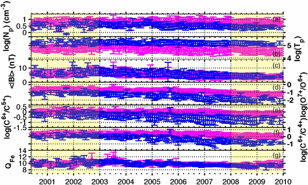
Figure 5. Plasma parameters and solar wind ion charge state indicators are shown. Slow solar wind data is shown in magenta and fast wind data is shown in blue in each of the panels. Panel (a) shows the Carrington rotation averaged proton density (Np), (b) proton kinetic temperature (Tp), (c) the magnetic field magnitude 〈|B|〉, (d) O7+/O6+, (e) C6+/C5+, f) C6+/C4+, and (g) QFe. All quantities are shown as log values, with the only exceptions being 〈|B|〉 and QFe.
Download figure:
Standard image High-resolution image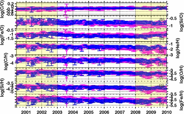
Figure 6. Carrington rotation averaged elemental abundances relative to O and H are shown. Slow solar wind data is shown in magenta and fast wind data is shown in blue in each of the panels. Panel (a) shows C/O, and (b) and (c) show Si/O and Fe/O, respectively. Panels (d)–(h) show the abundance of a specific heavy ion as compared to the protons and for increasing mass from He, C, O, Si, to Fe. All quantities are shown as log values.
Download figure:
Standard image High-resolution imageIn Figure 5, slow solar wind data are shown in magenta and fast wind data are shown in blue in each of the panels. Panel (a) shows the average proton density (Np), and (b) shows the proton kinetic temperature (Tp), identical to those shown Figures 3 and 4, respectively. The magnetic field magnitude, 〈|B|〉, is shown in panel (c) from ACE/MAG. The bottom four panels show three ionic charge states often used as proxies for near-solar temperatures (d) O7 +/O6 +, (e) C6 +/C5 +, and the best near-solar proxy (f) C6 +/C4 + Landi et al. 2012a). We also show the average Fe charge state QFe in panel (g), which is a good temperature proxy for the far corona (Buergi & Geiss 1986). All quantities are shown as log values, with the only exceptions of 〈|B|〉 and QFe.
While there are some periods with a significant degree of variability in all observed plasma and compositional measurements from one Carrington rotation to the next, long-term trends are evident in both the fast and slow solar wind, with some significant changes between fast and slow wind. During solar maximum (from approximately the beginning of 2000 until the end of 2002), there are significantly higher ionic charge states (O7 +/O6 +, C6 +/C5 +, C6 +/C4 +) and also slightly higher Fe/O abundances, especially in slow wind. Both plasma density and proton temperature appear higher during solar maximum as compared to solar minimum, as does the average magnetic flux density 〈|B|〉. There is an indication of a trend toward higher values for some compositional and plasma parameters near the end of 2009, as solar cycle 24 began.
Carrington rotation averages of all the bulk parameters of the fast and slow solar wind (proton temperature and density, magnetic field) show some decrease from solar maximum to solar minimum, even accounting for some variability of the fast solar wind at maximum. The most notable exception is the proton density of the slow wind, which does not show any significant change over almost one full solar cycle. On the contrary, the fast wind proton density changes significantly between at least 2003 and 2010, with most of the change occurring between 2004 and 2006 (McComas et al. 2008). The rise of cycle 24 does not seem to alter the wind density significantly in 2010.
The 2004–2006 period also seems to show the largest changes in the slow wind proton temperature, which decreases by a factor approximately 1.5 and then very slowly continues to decrease as the Sun enters the minimum phase. On the contrary, the fast wind proton temperature shows a much more moderate decrease, which takes place very gradually with time. Both the fast and slow solar wind magnetic field show a marked, steady decrease with time from the maximum value reached at around 2003; reaching almost a factor two difference in 2009 as compared to the average early in the cycle. The start of solar cycle 24 does not seem to affect the wind magnetic field, as of 2010.
During solar maximum (from approximately the beginning of 2000 until the end of 2002), there are significantly higher ionic charge states (O7 +/O6 +, C6 +/C5 +, C6 +/C4 +) and also slightly higher Fe/O abundances, especially in slow wind. Both C and O show a large decrease in their ionization distribution toward solar minimum. The slow solar wind dropped to less than 30% of the solar maximum value for O7 +/O6 +. This is likely due to the fact that O6 + became, by far, the most abundant ion during solar minimum reflecting overall changes in the coronal electron temperature and density. Both C6 +/C5 + and C6 +/C4 + dropped, and drastically so in the fast wind, with the value of C6 +/C4 + dropping to less than 20% of what it was at solar maximum. The QFe values did not change much over the solar cycle or across solar wind types. There is an indication of a trend toward higher values for some compositional and plasma parameters near the end of 2009, as solar cycle 24 began.
Figure 6 shows the long-term evolution of elemental abundances of heavy ions over the same mission period. Again the parameters are separated into slow (magenta) and fast (blue) solar wind types, ICMEs are removed, and Carrington rotation averages and standard deviations are calculated the same way as in Figure 5. All quantities are shown as log values.
Element abundance ratios are obtained using total element densities of H, He, C, O, Si, and Fe measured by ACE/SWICS. For each element, the total density is calculated by summing the densities of all individual charge states that show significant counts: these are C4 + to C6 + for carbon, O5 + to O8 + for oxygen, Si6 + to S12 + for silicon and Fe6 + to Fe20 + for Iron. Helium is almost entirely in its fully ionized state so we only considered this ion, He2 +, and of course, H is only H+. Figure 6(a) shows C/O, and (b) and (c) show Si/O and Fe/O, respectively. Panels (d)–(h) show the abundance of a specific heavy ion as compared to the protons and for increasing mass from He, C, O, Si, to Fe.
We begin by discussing the elemental ratios relative to O, which have been shown to be organized by FIP and examine the evolution of the solar wind FIP bias over the solar cycle. Geiss et al. (1995) showed that the Fe/O ratio was different between the fast and the slow solar wind, and noted that this ratio was affected by the same fractionation effects which are present in the lower solar corona, known as FIP effect. The FIP effect consists of the systematic increase in the abundance ratio between an element with FIP smaller than 10 eV (low-FIP element) to an element with FIP larger than 10 eV (high-FIP element), relative to the same abundance ratio in the photosphere (Feldman 1992; Feldman & Laming 2000). The amount of enhancement of the low-FIP/high-FIP ratio from its photospheric value is called "FIP bias." In Figure 6, we show two low-FIP elements (Si, Fe) and two high-FIP elements (C, O). Both the fast and slow wind FIP ratios evolve significantly from solar maximum to solar minimum. The He/O ratio (not shown) behaves differently from the other elements and a large difference tends to develop between the fast and slow solar wind at solar minimum: the slow wind becomes much more depleted in He/O at solar minimum (as will be discussed in Section 7). C/O behaves in the same way in both the fast and slow solar wind, as expected of these two elements, which both belong to the high-FIP class. However, there is an interesting trend in the C/O data that is not evident in any other data: C/O slightly increases toward solar minimum, unlike any of the other elemental abundance ratios, even though that increase is only marginally significant if compared with the error bars. This behavior merits further consideration, which is beyond the scope of the current paper, as these two elements belong to the same FIP class and thus, in the standard picture of the FIP effect, are expected to behave in the same way. Si/O becomes steadier in the fast wind and Si decreases in abundance relative to O toward solar minimum, with the slow wind abundance dropping more significantly than the fast wind abundance, although the variations in the slow wind are very large. The Si/O ratio behaves differently from the Fe/O ratio, which appears to drop to lower levels in the fast wind and is equally steady in both the fast and slow wind. These differences are unexpected since both ratios are indicators of the FIP bias, and since Fe and Si also belong to the same FIP class they are expected to behave in the same way in the standard FIP scenario.
We also measured the heavy ion abundances relative to H. Comparisons with H enable us to examine whether there are mass dependent changes in the selection of solar wind as it is accelerated out of the corona (e.g., Raymond et al. 1997; Weberg et al. 2012). There is a general trend in both the fast and slow wind, which shows all the ratios dropping from solar maximum to solar minimum, although the fast wind at solar maximum is quite variable. In all of the ratios, the slow wind drops to the lowest values at the absolute minimum in the end of 2008. While the slow wind shows less variability throughout, the fast wind becomes quite steady across Carrington rotations toward solar minimum.
6. TEMPORAL EVOLUTION OF FAST AND SLOW WIND
In this section, we briefly discuss the evolution of the solar wind with time, as shown by Figures 5 and 6. To help quantify our analysis, we have reported in Table 1 the average values (with their variability as defined with Figure 2) of all the parameters calculated over the lognormal distribution of each of the parameters. These averages have been taken over the 2000–2002 period for the solar maximum and 2008–2009 period for solar minimum as highlighted in Figures 5 and 6.
Table 1. The Average Values for the Fast and Slow Wind and Their Upper and Lower Limits (See Text for More Details) Calculated over the Lognormal Distribution of Each of the Parameters in This Study
| Parameter | Solar Max | Solar Max | Solar Min | Solar Min | ||||||||
|---|---|---|---|---|---|---|---|---|---|---|---|---|
| Slow | Fast | Slow | Fast | |||||||||
| Lower | Mean | Upper | Lower | Mean | Upper | Lower | Mean | Upper | Lower | Mean | Upper | |
| np | 3.28E+00 | 6.13E+00 | 1.15E+01 | 2.01E+00 | 3.44E+00 | 5.87E+00 | 2.93E+00 | 5.42E+00 | 1.00E+01 | 1.70E+00 | 2.56E+00 | 3.86E+00 |
| Tp | 2.93E+04 | 5.74E+04 | 1.13E+05 | 1.08E+05 | 1.68E+05 | 2.61E+05 | 1.93E+04 | 3.80E+04 | 7.46E+04 | 1.03E+05 | 1.49E+05 | 2.18E+05 |
| |B| | 4.13E+00 | 6.03E+00 | 8.79E+00 | 4.52E+00 | 6.38E+00 | 9.01E+00 | 2.33E+00 | 3.56E+00 | 5.44E+00 | 3.18E+00 | 4.31E+00 | 5.85E+00 |
| O7/O6 | 1.19E−01 | 2.29E−01 | 4.41E−01 | 3.44E−02 | 6.47E−02 | 1.21E−01 | 2.89E−02 | 6.07E−02 | 1.28E−01 | 6.02E−03 | 1.31E−02 | 2.85E−02 |
| C6/C5 | 5.27E−01 | 1.02E+00 | 1.98E+00 | 2.83E−01 | 4.86E−01 | 8.35E−01 | 3.83E−01 | 6.71E−01 | 1.18E+00 | 1.06E−01 | 1.83E−01 | 3.14E−01 |
| C6/C4 | 1.18E+00 | 2.46E+00 | 5.12E+00 | 5.67E−01 | 1.12E+00 | 2.19E+00 | 5.35E−01 | 1.25E+00 | 2.94E+00 | 9.20E−02 | 1.99E−01 | 4.30E−01 |
| QFe | 9.05E+00 | 9.94E+00 | 1.08E+01 | 9.43E+00 | 1.03E+01 | 1.12E+01 | 8.71E+00 | 9.55E+00 | 1.04E+01 | 8.73E+00 | 9.19E+00 | 9.64E+00 |
| He/O | 5.32E+01 | 7.63E+01 | 1.09E+02 | 6.88E+01 | 8.57E+01 | 1.07E+02 | 3.05E+01 | 4.81E+01 | 7.59E+01 | 6.16E+01 | 8.00E+01 | 1.04E+02 |
| C/O | 4.84E−01 | 6.34E−01 | 8.29E−01 | 6.02E−01 | 6.86E−01 | 7.80E−01 | 6.02E−01 | 7.36E−01 | 9.00E−01 | 6.41E−01 | 7.09E−01 | 7.83E−01 |
| Si/O | 1.24E−01 | 1.65E−01 | 2.20E−01 | 1.12E−01 | 1.66E−01 | 2.45E−01 | 8.17E−02 | 1.26E−01 | 1.93E−01 | 1.30E−01 | 1.63E−01 | 2.03E−01 |
| Fe/O | 6.19E−02 | 1.01E−01 | 1.63E−01 | 4.57E−02 | 7.29E−02 | 1.16E−01 | 4.71E−02 | 8.37E−02 | 1.49E−01 | 3.75E−02 | 5.23E−02 | 7.29E−02 |
| He/H | 1.93E−02 | 3.63E−02 | 6.82E−02 | 1.44E−02 | 2.84E−02 | 5.61E−02 | 2.98E−03 | 9.59E−03 | 3.08E−02 | 1.12E−02 | 2.05E−02 | 3.74E−02 |
| C/H | 1.64E−04 | 3.02E−04 | 5.56E−04 | 1.18E−04 | 2.27E−04 | 4.40E−04 | 6.21E−05 | 1.51E−04 | 3.70E−04 | 1.10E−04 | 1.81E−04 | 3.00E−04 |
| O/H | 2.62E−04 | 4.76E−04 | 8.63E−04 | 1.80E−04 | 3.32E−04 | 6.11E−04 | 8.21E−05 | 2.03E−04 | 5.04E−04 | 1.61E−04 | 2.56E−04 | 4.06E−04 |
| Si/H | 4.16E−05 | 7.87E−05 | 1.49E−04 | 2.94E−05 | 5.51E−05 | 1.03E−04 | 1.01E−05 | 2.66E−05 | 7.01E−05 | 2.44E−05 | 4.16E−05 | 7.10E−05 |
| Fe/H | 2.18E−05 | 4.81E−05 | 1.06E−04 | 1.09E−05 | 2.44E−05 | 5.43E−05 | 6.64E−06 | 1.81E−05 | 4.91E−05 | 7.31E−06 | 1.34E−05 | 2.44E−05 |
Download table as: ASCIITypeset image
We will first discuss the evolution of the fast and slow solar wind separately, and compare their evolution tracks to highlight their differences and similarities. Next, we will compare the characteristics of the fast and slow solar wind at minimum and at maximum.
6.1. Thermodynamic Properties
The changes described above for Figure 5 point toward a decreased ionizing capability of the solar wind close to the Sun before freeze-in occurs. Such a change is far more pronounced in the fast solar wind, where it reaches one order of magnitude in all charge state ratios shown in Figure 5, than in the slow solar wind, where it is a factor of 2–3 at maximum. Since C and O freeze-in within 1.5–1.6 solar radii (e.g., Landi et al. 2012a, and references therein) such a large decrease indicates that both types of wind experience a fairly different evolution in the regions closest to their source at solar maximum and at solar minimum; also, differences are more dramatic for the fast wind than for the slow wind. On the contrary, the decrease in the average charge state of iron QFe, shown in the bottom panel of Figure 5, is the same for both types of wind and is rather limited, although the large variability experienced at solar maximum makes it difficult to quantify the amount of decrease. Since Fe freezes-in at larger heights than C and O (between 1.5 and 4.0 solar radii; see Landi et al. 2012a and references therein), this behavior shows that the ionization history of both winds is similar in the extended corona, and that the effect of the solar cycle on it is limited. Moreover, QFe seems to be sensitive to specific physical conditions prevalent during the beginning of solar cycle 24, as shown by the sudden increase at the beginning of 2009. It is also is interesting to note that the absolute value of QFe is nearly identical, within error bars, for both winds at least from 2003 to 2010. This seems to suggest that the differences between fast and slow solar wind are mostly generated in the low corona, where C and O freeze-in, and then the two winds experience a similar evolution in the extended corona, where Fe freezes-in.
In summary, Figure 5 shows that the evolution of the fast and slow solar wind over the solar cycle is rather distinct and different as far as the thermodynamic properties of the protons are concerned, with the slow wind cooling but approximately maintaining its mass flux while the fast wind becomes more rarefied but limits the decrease in temperature. Also, while both wind types exhibit dramatic decreases in the charge state ratios of the lightest elements, the degree to which each changes is different. The behavior of Fe is the same for both winds, and the solar cycle effect on this element is more moderate. Since the solar wind ionization state is largely determined by the electron density and temperature, this indicates (1) a significant change in the thermodynamic properties of the electrons in the low corona occurs as the solar cycle evolves, (2) that the degree of change is different for each type of wind, and (3) cycle-induced changes decrease significantly at larger altitude where Fe is still evolving and C and O are already frozen-in.
6.2. Compositional Characteristics over Time
Figure 6 shows the evolution of the composition of both solar winds with time. The first thing to notice is that both types of winds evolve in the same qualitative way, indicating that the solar cycle influences the composition of the source regions of both types of wind in a similar way.
The second thing to notice is that the FIP bias evolution as indicated by the Si/O ratio and the Fe/O ratios are significantly different from each other, beyond the statistical and systematic limits of the SWICS instrument. While the overall FIP bias evolution indicated by Si/O shows a steady decrease from minimum to maximum and does not seem to notice the beginning of Cycle 24, the evolution shown by Fe/O presents a marked increase after 2008. Additionally, the Si/O ratio decreases less in the fast wind than in the slow wind while the opposite is true for Fe/O. In the fast wind, Fe/O drops more than in the slow. Since no particular difference in the FIP bias behavior of Si and Fe is found from spectroscopic observations of the lower corona, such a difference has to be introduced at larger altitudes than can be observed by current remote sensing instrumentation, i.e., beyond 1.5 solar radii.
Most importantly, all abundances of heavy elements relative to H+, including He/H, decrease steadily and significantly. Even though variability at solar maximum for both winds makes it difficult to quantify such a decrease on a time by time basis, the decreasing trend is obvious and beyond the uncertainties of the data. The depletion reaches its maximum in late 2008, when all elements drop in concert with one another. Afterward, the beginning of solar cycle 24 brings a slight increase in the abundances before the end of the study period.
6.3. On the Discrimination between Fast and Slow Solar Wind
Since the fast and slow solar wind are observed to evolve differently with the solar cycle, the art of discriminating between the two solar wind types using a single parameter will depend on the behavior of that parameter during that phase of the solar cycle.
Until now, the main parameters used to discriminate between fast and slow solar wind are typically hard cutoffs in (1) bulk speed, (2) Fe/O ratio, and (3) O7 +/O6 + ratio. Recently, Landi et al. (2012a) showed that the C6 +/C4 + ratio could be a more effective indicator of solar wind type, but it provides a similar qualitative type of indication to the O7 +/O6 + ratio, as charge state ratios respond to the evolution in the electron properties. The question is, are any of the above parameters valid indicators of solar wind type at any time irrespective of the phase of the solar cycle. To answer this question, we need to look at the evolution of element abundance ratios and charge state ratios with time as shown in Figures 5 and 6, bearing in mind that these figures have been constructed using velocity as a divisor between fast and slow solar wind within each Carrington rotation.
The first thing to notice is that even though for a given time in the solar cycle, ionic charge state ratios such as C6 +/C4 + are powerful discriminators between the types of wind, there is not one single value that robustly applies as a discriminator during the entire solar cycle analyzed here. In fact, while at any given moment during the cycle the charge state ratios of the slow solar wind are larger than those in the fast wind, the values of these ratios in the slow wind at solar minimum are the same as those of the fast wind at solar maximum. This renders the challenge impossible to build a strict and temporally independent selection criteria based on the absolute value of charge state ratios. Such a criterion needs to take into account the phase of the solar cycle. This conclusion affects all the most commonly used charge state ratios, which we have shown in Figure 5.
Thermodynamic properties of the protons do show a clear difference between fast and slow wind when separated by wind speed. The fast wind protons always have a larger temperature and a lower density than the slow wind protons. However, since the wind density falls off with radial distance from the Sun, a selection criteria based on density would not be valid throughout the heliosphere at various past, present, and future spacecraft located at different heliocentric distances. The proton temperature appears to be a very useful parameter, as the range of values reached by each type of wind is sufficiently separated at any time in the cycle to be used as a marker of wind type. This is likely due to the positive correlation of the proton temperature and proton velocity reported since the Helios era (e.g., Lopez & Freeman 1986; Freeman & Lopez 1987). Hence, the proton temperature differences tend to mirror the differences in the solar wind speed for the two types of wind here. One could easily have found the same behavior of the solar wind had they separated the wind by proton temperature instead of speed. Figure 7 shows the correlation for the proton velocity and proton temperature from ACE with the separator in solar wind speed at 500 km s−1 shown as the vertical green dashed line. The same flattening above 500 km s−1 is apparent here as was described in Lopez and Freeman (1986). The thermal properties of protons in the inner heliospheric solar wind are strongly affected by turbulence properties of the magnetic field in the near and far corona (Marsch & Schwenn 1990 and references therein). The distinct differences of the dissipative character of the solar wind magnetic turbulence seem to be retained during the entire solar cycle. Note, however, that there are important limitations of velocity and temperature measures, as they can be affected by in situ evolutionary processes.

Figure 7. Correlation of the proton velocity and proton temperature from ACE with the separator in solar wind speed at 500 km s−1 shown as the vertical green dashed line.
Download figure:
Standard image High-resolution imageNot even elemental abundance ratios can provide a discriminator of solar wind type that can be used at all times during the solar cycle. While the FIP bias as indicated by the Fe/O ratio has been suggested as a marker, Figure 6 shows that a significant evolution of such a ratio prevents the development of a universally valid criterion. In fact, even if the Fe/O ratio in the slow solar wind is larger than in the fast solar wind at any given time during the cycle, the Fe/O ratio value of the slow wind at solar minimum is even smaller than the fast wind Fe/O ratio value at solar maximum. This is somewhat in contrast with high-latitude results which found no or little evidence of elemental composition evolution over the solar cycle (von Steiger et al. 2000; von Steiger & Zurbuchen 2011), but precludes the use of such parameter as a universal marker of wind type.
7. DISCUSSION
The observed reduction of plasma density, temperature, and magnetic field flux density has been previously discussed by McComas et al. 2008; Smith & Balogh 2008) and is presumably related to coronal processes and a reduced outflow of mass and magnetic flux from the Sun. For example, based on scaling laws, Schwadron & McComas (2003) have suggested that the underlying reason for both plasma and ionic compositional changes (indicated by O7 +/O6 + in their work) are caused by a difference of magnetic emergence rates near the Sun. Our analysis of C6 +/C4 +, the best proxy for coronal temperatures of the low corona, shows an even more dramatic decrease, especially for slow wind. These ionic charge state decreases occur in all C and O ratios plotted and for fast and slow wind. A look at the ion ratios show that the fast wind dropped to much lower values than the slow wind at solar minimum or even the fast wind at solar maximum. For fast wind, the decreases are comparable with the ones measured at high latitudes during four Ulysses passes (von Steiger & Zurbuchen 2011). The decrease of QFe occurs concurrently within fast and slow wind, indicating the useful measure of QFe as an outer corona temperature proxy.
A look at the ion ratios show that the fast wind dropped to much lower values than the slow wind at solar minimum or even the fast wind at solar maximum. The slow wind at solar minimum looked much more similar to the fast wind at solar maximum based on the ion charge state ratios. These changes indicate a global shift towards lower charge states and a more intense shift in the coronal hole regions. These findings are consistent with some of the conclusions of Kasper et al. (2012), Schwadron et al. (2011), and McIntosh et al. (2011), who interpreted these changes as a cooling of the corona. Von Steiger & Zurbuchen (2011) examined solar wind from polar coronal holes on Ulysses and found that the charge states dropped significantly in the holes from the solar minimum of cycle 22 versus cycle 23. They suggest that this reduction is likely not explained by a reduction in the density profile, but instead by an overall cooling of the polar corona.
While a drop in the charge state ratio is generally interpreted as a drop in the electron temperature in the corona, the frozen-in charge state reflects not only the electron temperature, but also the electron density in the freeze-in region and the velocity with which the ions flow out through this ionization region. E. Landi & P. Testa (2013, in preparation) report that spectroscopic temperatures of streamers (slow wind) have not changed significantly over the solar cycle within the error bars of their investigation (∼15%), thus it is unlikely that purely a drop in the coronal electron temperature can explain the reduction in the charge states of the slow wind. It is most likely here, in light of these measurements, that the coronal density is in fact lower and hence, the wind, starting from low ionization states lower in the corona (below the temperature maximum) has a decreased ability to ionize, resulting in lower final charge states. This density reduction must be confined to the low corona since QFe is mostly unaffected over the solar cycle.
The changes in the elemental abundances relative to O are put into context with measurements from von Steiger et al. (2000). In order to consider whether there are any significant changes to the FIP ordering, we plot the FIP abundances relative to the photospheric abundances from Grevesse & Sauval (1998). Figure 8 compares and contrasts the findings from von Steiger et al. (2000) from Ulysses from the solar maximum in 1991–1992, and solar minimum in 1994–1996 with our findings in the ecliptic. Figure 8(a) shows the comparison with our ACE slow wind values at solar maximum with the values from von Steiger et al. (2000) denoted by "RVS." The FIP bias appears to be the same during the solar maximum of cycle 23 as it was for the cycle 22. Figure 8(b) shows the comparison of ACE solar minimum slow wind values with those from cycle 22; again the FIP bias behavior looks the same within the error bars. Figure 8(c) shows the comparison of the fast wind values from ACE and RVS at solar minimum. Here there are some deviations during the latest minimum. Si/O is further enhanced over photospheric values much beyond the von Steiger et al. (2000) values. And Fe/O looks even more photospheric in the ACE data. McIntosh et al. (2011) also found a drop in the Fe/O ratio during the latest solar minimum and reported that it is likely due to the fact that the supergranule length scale has decreased, thereby reducing the particle density and energy flux which is available to heat the fast wind. Aside from the fast solar wind, which is not highly affected by FIP, the slow solar wind appears to retain a very similar FIP bias over the entire solar cycle, despite the large changes in ionization states and even the depletion of heavy ions relative to H.

Figure 8. Comparison of FIP bias of elemental abundances compared to findings from von Steiger et al. (2000) from Ulysses from the solar maximum in 1991–1992, and solar minimum in 1994–1996. Panel (a) shows the comparison with our ACE slow wind values at solar maximum, von Steiger et al. (2000) values are labeled "RVS." Panel (b) shows the comparison of ACE solar minimum slow wind values with those from cycle 22. The slow wind FIP bias behavior looks similar to that of von Steiger et al. (2000) within the error bars. Panel (c) shows the comparison of the fast wind values from ACE and RVS at solar minimum, Fe/O and Si/O deviate from values found by von Steiger et al (2000).
Download figure:
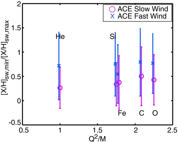
Standard image High-resolution imageExamination of the elemental abundances relative to H showed a reduction in heavy ions in both solar wind types from solar maximum to solar minimum. Our values for AHe are consistent with those from Kasper et al. (2012), who found that the AHe variations are strongly correlated to the solar wind speed at speeds less than 450 km s−1. The AHe variation is correlated with solar activity as suggested by Aellig et al. (2001), who suggested that lower helium abundances were a result of less efficient Coulomb drag. A comparison of the ratios of the maximum to minimum values of the heavy ion abundances relative to H versus the collisionality term, Q2/M, for the fast and the slow wind is shown in Figure 9 with error bars propagated from Table. The error bars are very large since the variability in the wind is large, however, the drop in the values between maximum and minimum is still a measurable effect. Any indication of a charge to mass dependent depletion, indicative of collisional coupling, of heavy ions in the solar wind at solar minimum is obfuscated by the large error bars, hence we must conclude that the drop for all heavy ions, while real, is of approximately the same order.
Figure 9. A comparison of the ratios of the maximum to minimum values of the heavy ion abundances relative to H vs. the collisionality term, Q2/M, for the fast (blue) and the slow (magenta) wind. The error bars are very large since the variability in the wind is large, however, the drop in the values between maximum and minimum is still a measurable effect. The drop for all heavy ions is of approximately the same order within the constraints of the error bars.
Download figure:
Standard image High-resolution image
The elemental abundances of heavy ions relative to H drop to a comparable fraction irrespective of solar wind type (as shown in Figure 9), with the slow wind becoming slightly more depleted than the fast wind. We can consider this preferential depletion of heavy ions in the context of predictions from Geiss et al. (1970), where the collisionality term is proportional to density and proportional to T−3/2, where T is the ion or proton temperature. If we presume that the collisional coupling between the protons and heavy ions becomes less efficient over the solar cycle, that could indicate that the ion and proton temperatures increased in the corona. Unfortunately, we cannot verify this prediction since observations of the proton temperature in the corona remain elusive; also, the only measurement of heavy ion temperatures as a function of time in the quiet corona was done by Landi (2007) during the rising phase of the solar cycle and showed no sign of cycle-related change. Alternately, findings from von Steiger & Zurbuchen (2011) state that in polar coronal holes, the electron temperature and the density decreased; this density drop may dominate the collisional coupling term and therefore modify the heavy ion abundances in the solar wind. E. Landi & P. Testa (2013, in preparation) find that the electron temperature remains approximately constant over time in the corona, so, if the ion and electron temperatures are essentially equal, the drop in density may explain the reduced collisional coupling efficiency. A drop in proton density is also supported by the observed reduction in the proton mass flux in the heliosphere during the most recent solar minimum (McComas et al. 2008).
There is a large body of literature regarding abundance variations in the corona, especially that of He. For example, Hansteen et al. (1994) found in their models that when the coronal temperature is reduced below a certain limit, reducing the proton flux out of the corona and thus reducing the drag on the alpha particles, helium can build up in the corona and could become depleted in the solar wind. Alternately, increased coronal temperatures and the associated enhanced proton flux can drag more helium into the corona as well, which will in turn increase drag on the protons flowing out into the solar wind, however, this would serve to enhance the heavy ion relative abundance. Byhring et al. (2011) modeled Fe abundance enhancements in the solar wind and found that heavy ions will also pile-up in the corona due to reduced proton fluxes as observed during eclipses. Hence, the reduced densities and/or temperatures in the corona, and therefore reduced solar wind proton fluxes during the recent solar minimum may result in a reduction in the heavy ions that make it out into the solar wind. This could also be achieved through a solar cycle dependence of one of the physical quantities, such as waves and turbulence fields, that accelerates the solar wind and couples the heavy ions to the protons.
The fact that the heavy ion abundances drop at solar minimum for both solar wind types suggests that there are global changes either in the processes that accelerate the wind or in the properties of loops releasing plasma into the wind. Evidence supports a reduced proton flux in the corona, which in turn is less effective at accelerating heavy ions out of the corona. The reduction in the ion charge states indicates changing thermodynamic properties of electrons in the low corona.
8. SUMMARY
Our analysis of solar wind heavy ion composition over solar cycle 23 has revealed insight into the behavior of the corona and processes that accelerate the wind. In particular, solar wind heavy ion composition reveals how corona properties, such as electron temperature, density, and ion outflow velocities in the source region of the wind evolve. We can use these measurements to determine the conditions in the solar wind source region.
Our key findings can be summarized as follows.
- 1.Indicators of solar wind type must be chosen carefully.
- a.While heavy ion charge state ratios and average charge states are excellent local identifiers of changes in solar wind source within a Carrington rotation, or even across a given year, they cannot be used as an absolute discriminator of solar wind source across the entire solar cycle as the values evolve considerably across the solar cycle.
- b.Elemental composition has also been shown to be an excellent local indicator of solar wind source and can be used to examine the evolution of the source regions and the acceleration processes within them over time. However, elemental composition also cannot be used as an absolute discriminator of solar wind source between difference phases of the solar cycle as the values evolve considerably throughout.
- c.Using solar wind velocity or even the proton temperature to discriminate between different types of solar wind can be an effective method as the velocity and kinetic temperature are quite different in the coronal hole and streamer wind throughout the entire solar cycle. Together, with heavy ion composition, the physical nature of solar wind sources can be characterized.
- 2.The FIP bias in the fast solar wind evolves over the solar cycle indicating that properties of the source plasma change. While Si/O becomes more photospheric, Fe/O at solar minimum evolves to resemble the more FIP-enhanced slow wind. The FIP bias in the slow solar wind does not evolve appreciably.
- 3.Charge state ratios in both the fast and slow wind decrease from solar maximum to solar minimum indicating that the properties of the free electrons in the low corona change. It is also likely that the density in the low corona decreases toward solar minimum.
- 4.Both the fast and slow wind become more depleted of heavy ions at solar minimum, although the slow wind becomes more depleted. There may be a weak charge to mass dependence of this depletion, although this is mostly obscured by the large degree of variability of the abundances of heavy ions relative to H.
- 5.The fast solar wind experiences the largest changes in charge state composition and small changes in elemental composition while the slow wind experiences large changes in both.
S.T.L. and T.H.Z. are supported by NASA grants NNX10AQ61G and NNX08AI11G. E.L. is supported by the NNX11AC20G and NNX10AQ58G NASA grants, and by NSF grant AGS-1154443.