


ABSTRACT
The coronal magnetic field is of paramount importance in solar and heliospheric physics. Two profoundly different views of the coronal magnetic field have emerged. In quasi-steady models, the predominant source of open magnetic field is in coronal holes. In contrast, in the interchange model, the open magnetic flux is conserved, and the coronal magnetic field can only respond to the photospheric evolution via interchange reconnection. In this view, the open magnetic flux diffuses through the closed, streamer belt fields, and substantial open flux is present in the streamer belt during solar minimum. However, Antiochos and coworkers, in the form of a conjecture, argued that truly isolated open flux cannot exist in a configuration with one heliospheric current sheet—it will connect via narrow corridors to the polar coronal hole of the same polarity. This contradicts the requirements of the interchange model. We have performed an MHD simulation of the solar corona up to 20 R☉ to test both the interchange model and the Antiochos conjecture. We use a synoptic map for Carrington rotation 1913 as the boundary condition for the model, with two small bipoles introduced into the region where a positive polarity extended coronal hole forms. We introduce flows at the photospheric boundary surface to see if open flux associated with the bipoles can be moved into the closed-field region. Interchange reconnection does occur in response to these motions. However, we find that the open magnetic flux cannot be simply injected into closed-field regions—the flux eventually closes down and disconnected flux is created. Flux either opens or closes, as required, to maintain topologically distinct open- and closed-field regions, with no indiscriminate mixing of the two. The early evolution conforms to the Antiochos conjecture in that a narrow corridor of open flux connects the portion of the coronal hole that is nearly detached by one of the bipoles. In the later evolution, a detached coronal hole forms, in apparent violation of the Antiochos conjecture. Further investigation reveals that this detached coronal hole is actually linked to the extended coronal hole by a separatrix footprint on the photosphere of zero width. Therefore, the essential idea of the conjecture is preserved, if we modify it to state that coronal holes in the same polarity region are always linked, either by finite width corridors or separatrix footprints. The implications of these results for interchange reconnection and the sources of the slow solar wind are briefly discussed.
Export citation and abstract BibTeX RIS
1. INTRODUCTION
The "open" magnetic field is the portion of the Sun's magnetic field that stretches out into the heliosphere to become the interplanetary magnetic field (IMF). It defines the structure of the heliosphere, including the position of the heliospheric current sheet (HCS) and the regions of fast and slow solar wind.
The most obvious source of open magnetic flux on the Sun is coronal holes (Wang et al. 1996). These are regions of the solar corona that appear dark in X-ray emission (Zirker 1977) and bright in He i 10830 Å absorption (Zirker 1977; Harvey & Sheeley 1979), and are believed to be the source of the fast solar wind. While the sun and the solar wind exhibit a variety of dynamic phenomena on a multitude of time and spatial scales, the large-scale underlying structure of the corona often varies slowly near solar minimum, as evidenced by the recurrent patterns of coronal holes and fast solar wind streams (Zirker 1977; Luhmann et al. 2009; Abramenko et al. 2010). Using measurements of the photospheric magnetic field as input, steady-state models have been successful in reproducing features of the large-scale corona and inner heliosphere, such as the location of coronal holes, the streamer belt, and the HCS. The simplest and most widely available are the potential (current-free) magnetic field models, such as the potential field source-surface (PFSS) model (Schatten et al. 1969; Altschuler & Newkirk 1969) and the potential field current-sheet (PFCS) model (Schatten 1971). The models have been compared extensively with interplanetary observations (Hoeksema et al. 1983; Wang & Sheeley 1988, 1995; Zhao & Hoeksema 1995; Neugebauer et al. 1998). In conjunction with these magnetic field models, the inverse correlation between magnetic flux tube expansion and solar wind speed has been used to predict solar wind speeds in the heliosphere (Wang & Sheeley 1990, 1994; Wang et al. 1997; Arge & Pizzo 2000; Arge et al. 2003). Magnetohydrodynamic (MHD) models of the solar corona have also been used (Usmanov 1993; Mikić & Linker 1996; Usmanov 1996; Linker et al. 1999; Mikić et al. 1999; Riley et al. 2001; Roussev et al. 2003); the models are time dependent, but are advanced in time to obtain a steady-state solution. MHD models provide a more self-consistent description of the plasma and magnetic fields, but in practice many of the features of the solutions are similar to source-surface models (Riley et al. 2006). MHD models with a more realistic description of the energy transport have now been developed (Lionello et al. 2009) that allow direct comparison with emission measurements in the corona.
Despite the success of steady-state descriptions, a number of observations imply that important phenomena involving the Sun's open flux are inherently dynamic in nature. For example, observations of the first ionization potential (FIP; Geiss et al. 1995) show enhanced low FIP elements in the slow wind (the so-called FIP effect) but not in the fast wind, implying a different origin for the fast and slow wind plasma. Zurbuchen et al. (1998) and Schwadron et al. (1999) have described a possible FIP fractionation process occurring in closed loops that could explain the FIP effect as a consequence of the slow wind arising from previously closed large-scale loops. This implies that reconnection is necessary for the release of slow wind plasma (although see Cranmer et al. 2007 for an alternative explanation). White-light observations from the LASCO coronagraph reveal blobs of plasma escaping from the tips of streamers as well as downward flows (Wang et al. 2000; Sheeley & Wang 2002; Sheeley et al. 2009); observations from the STEREO Heliospheric imagers show evidence of plasma blobs in the more distant solar wind (Rouillard et al. 2008, 2010a) with associated in situ signatures (Rouillard et al. 2010b). All of these observations generally imply that plasma on previously closed-field lines escapes into interplanetary space.
It is not surprising that even on a large scale, the Sun's open flux is dynamic. It is well known that the photospheric magnetic flux is constantly evolving, even during solar minimum. Leighton (1964) first recognized the important role of both differential rotation and random-walk motions caused by the supergranule circulation in the reversal of the Sun's polar magnetic field during the 11 year sunspot cycle. Based on these concepts, flux evolution models (Devore et al. 1984; Sheeley et al. 1987; Wang & Sheeley 1991; Worden & Harvey 2000; Schrijver & DeRosa 2003) have been successful in reproducing many of the observed properties of photospheric fields.
The question of how the coronal magnetic field responds to photospheric flux evolution is a longstanding one. It was recognized very early that at times, the coronal field must respond to photospheric motions or the emergence of new flux by reconnection (Sheeley et al. 1975a, 1975b, 1989). Recently, diverging viewpoints have emerged between the solar and heliospheric communities in terms of the nature of this response, and in particular, the types of magnetic reconnection that are allowed (Zurbuchen 2007). In the solar physics community, sequences of source-surface models are often used to approximate the evolution of the coronal field in response to changes in the photospheric field (Wang et al. 1996; Wang & Sheeley 2004; Schrijver & DeRosa 2003; Wang & Sheeley 2004; Wang et al. 2010), assuming that the coronal field behaves in a quasi-steady manner. Wang et al. (1996) used this approach to explain the nearly rigid rotation of some coronal holes (Insley et al. 1995) in the presence of the differential rotation of the underlying photospheric magnetic flux (Newton & Nunn 1951). The results of this model imply reconnection and reconfiguration of the field. These processes are not directly calculated by the model, but they have been estimated (Wang & Sheeley 2004) and imply that both interchange reconnection and disconnection (discussed below) occur.
The heliospheric community has focused on the topology and structure of the magnetic field, which can be constrained by electron heat flux measurements. Table 1 summarizes the three principal ways that the coronal magnetic field can respond to photospheric evolution to maintain an extended coronal hole structure (as in Wang et al. 1996). In the first process, opening of the field leads to closed loops in the heliosphere. In the presence of minimal scattering, these field lines should exhibit counterstreaming electrons (referred to as a bidirectional heat flux). Counterstreaming electrons are most closely associated with coronal mass ejections (Gosling et al. 1990). On the other hand, the disconnection of field lines, which closes down flux, should lead to heat flux dropouts (McComas et al. 1989, 1991; again, if scattering is neglected). These events are rarely observed (Crooker et al. 2002). This has led heliospheric researchers to conclude that only the third process in Table 1, interchange reconnection, can occur. Based on this idea, Fisk and coworkers (Fisk et al. 1998, 1999; Fisk & Schwadron 2001; Fisk 2005; Fisk & Zurbuchen 2006) propose that open magnetic flux is approximately conserved, and that open field lines necessarily undergo a diffusive process through continual episodes of magnetic reconnection with neighboring closed loops. The concept of conservation of open flux has led to the idea of a "floor" in the interplanetary magnetic flux (Svalgaard & Cliver 2007; Owens et al. 2008). The most dramatic inference of this idea is that it implies that open flux must be transported into otherwise closed-field regions during its transequatorial migration that causes the reversal of the polarity of the solar magnetic field (Fisk & Schwadron 2001). Therefore, open flux should actually be present in the so-called closed-field regions of the streamer belt. For simplicity, we refer to this set of ideas in the rest of the paper as the interchange model.
Table 1. Coronal/Heliospheric Magnetic Field Processes
| Name | Process | Consequence | Observational Signature |
|---|---|---|---|
| (1) Field line opening | Closed loops are dragged out in the solar wind | Interplanetary flux increases | Bi-directional heat flux |
| (2) Disconnection | Two open-field lines reconnect | Interplanetary flux decreases | Heat flux drop outs |
| (3) Interchange reconnection | A closed-field line and an open-field line reconnect | Interplanetary flux is unchanged | Outward heat flux (usual interplanetary signature) |
Download table as: ASCIITypeset image
Recent observational and theoretical developments cast some doubt on this scenario. On the observational side, a re-interpretation of electron heat flux measurements by Owens & Crooker (2007) that accounts for scattering has shown that heat flux dropouts would be a rare occurrence even if disconnection events are present. Observations during the present unusual solar minimum (Smith & Balogh 2008) have shown that the IMF strength has dropped significantly, calling into question the idea that open flux is conserved and thus obviating the need to transport open flux through the closed-field regions. In theoretical work, Antiochos et al. (2007) have investigated the feasibility of open magnetic fields coexisting with surrounding closed flux. Using source-surface models, they argue heuristically for two conjectures regarding the structure of coronal holes. (1) Coronal holes are unique, in that every unipolar region on the photosphere can contain at most one coronal hole and (2) coronal holes of nested polarity regions must themselves be nested. As discussed in the paper, the practical consequence of these conjectures is that for a typical solar minimum configuration with one HCS, "isolated" coronal holes do not exist, they must be connected by narrow corridors that could be arbitrarily thin (and therefore not easily visible in emission). For brevity we refer to this main result as the Antiochos conjecture in this paper. If it is correct, open fields cannot simply diffuse into closed-field regions as required by the interchange model.
Time-dependent MHD simulations of the coronal response to photospheric motions can in principle follow the evolution of magnetic fields and help to resolve whether the quasi-steady model or the interchange model (or neither) is correct. MHD simulations of the coronal response to differential rotation (Lionello et al. 2005, 2006) find that interchange reconnection does occur, but the other processes in Table 1 happen as well. The MHD results generally support the conclusions of the quasi-steady models. However, the MHD models used large-scale flux distributions with unipolar coronal hole regions, with none of the small-scale opposite-polarity flux that is observed in coronal holes (this is true for most of the quasi-steady models as well). This might preclude the possibility of obtaining the results postulated by the interchange model.
In this paper, we describe MHD simulations designed to test two of the opposing ideas in the open flux debate. (1) Can open flux associated with small-scale polarities be advected into a closed-field region and remain open (as postulated by the interchange model)? (2) Can a portion of open flux be detached from a coronal hole (in contrast to the Antiochos conjecture)? We emphasize that these simulations are designed to test the response of weakly energized fields in the corona to a particular aspect of slow photospheric motions, and not the full breadth of behavior that the corona may exhibit when fields can emerge, cancel, or are near the threshold for eruption. Our study is similar in concept to the work of Edmondson et al. (2010), but with major enhancements. Unlike the previous study, we include a realistic photospheric magnetic flux distribution and an MHD treatment of the solar wind, so that open flux can be maintained rigorously by the plasma thermal and kinetic pressures. Furthermore, this allows us to calculate the full evolution at the HCS so that flux can open or close or undergo interchange reconnection there in response to the photospheric dynamics. In our simulation, we introduce two small bipoles into a smoothed synoptic map for Carrington rotation 1913. The bipoles are embedded in the area corresponding to the extended coronal hole that was observed during that time period. We first develop a global steady-state solution for the corona using this map as the boundary condition. We then impose a surface flow to advect these mixed polarities out of the coronal hole region, and study the evolution. We find that open magnetic flux associated with the northern bipole is not injected into the closed-field region, but closes down and disconnected flux is created in the heliosphere. Advection of the southern bipole leads to apparent detachment of a portion of the extended coronal hole. We find that the detached portion is in fact still linked to the main coronal hole by a zero-width separatrix surface. Investigation of the simulation results presented here spawned two other studies: Titov et al. (2011) designed an analytic model based on the simulation results to clarify the magnetic topology of isolated coronal holes. Antiochos et al. (2011) studied the results of high-resolution MHD simulations of the corona and discusses the implications of a web of separators and quasi-separatrix layers (QSLs) for interchange reconnection and the origin of the slow solar wind.
Section 2 of this paper describes the MHD model and the design and details of the simulations. Section 3 demonstrates the simulation results and discusses their implications. Our conclusions are presented in Section 4.
2. METHODOLOGY
To study the interaction of small-scale polarity magnetic bipoles with coronal holes, we use the MHD approximation, which is applicable to long-scale, low-frequency phenomena in magnetized plasmas such as the solar corona. Our model uses spherical coordinates and advances in time the following set of viscous and resistive MHD equations:
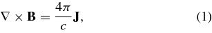
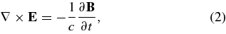
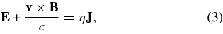
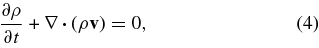
where B is the magnetic field, J is the electric current density, and E is the electric field. In practice the vector potential A is advanced, with B = ∇ × A. The variables ρ, v, p, and T are the plasma mass density, velocity, pressure, and temperature,  is the gravitational acceleration, η the resistivity, ν is the kinematic viscosity, and γ = 1.05 is the polytropic index. The polytropic approximation can be justified for the present study, since we are modeling the magnetic configuration of the corona and not the detailed properties of the plasma such as the contrast in speed between fast and slow wind, or coronal emission, for which a more sophisticated model would be necessary (Lionello et al. 2009). The boundary conditions are discussed by Linker & Mikić (1997) and Linker et al. (1999). We note that at the inner radial boundary, a fixed temperature of 1.8 × 10⁶ K and an electron density of 108 cm−3 are prescribed. The component of the velocity along the magnetic field is not specified but calculated from the characteristic equations. At the outer radial boundary the flow is supersonic and super-Alfvénic, and variables are computed with aid of the characteristic equations. For the simulation presented here, we have used a nonuniform grid in r × θ × ϕ of 151 × 191 × 291 points, with Δr ≈ 2.6 × 10⁻³ R☉ = 1.8 Mm at the lower radial boundary and Δr ≈ 0.75 R☉ at 20 R☉; the latitudinal mesh varies between Δθ ≈ 3
 7 at the poles and Δθ ≈ 05 near the equator. The azimuthal (longitudinal) mesh varies between Δϕ ≈ 05 in the primary region of study to Δϕ ≈ 30 further away. The simulation domain extends out to 20 R☉. The Alfvén travel time at the base of the corona (τA = R☉/VA) for |B| = 2.205 G and n0 = 108 cm−3, which are typical reference values, is 24 minutes (Alfvén speed VA = 480 km s-1). A uniform resistivity is chosen such that the Lundquist number SL = τR/τA is 1 × 10⁵, where τR is the resistive diffusion time. A uniform viscosity ν is also used, corresponding to a viscous diffusion time τν such that τν/τA = 500. Again, this value is chosen to dissipate unresolved scales without substantially affecting the global solution. During the phases of the simulation where reconnection occurs, the length scales are considerably smaller than 1RS and the numerical dissipation exceeds the specified η, so SL is consequently smaller in the regions where this dynamical evolution occurs.
A well-known problem for all MHD calculations of the solar corona is that SL of the corona (∼1013) is far greater than what is achievable with finite grid resolution in numerical simulations. Despite the large value of the coronal Lundquist number, there is ample evidence of magnetic reconnection in the solar corona (e.g., post-flare and post-CME loops), and all explanations for the quasi-rigid rotation of coronal holes involve reconnection. The problem of why reconnection occurs in highly conducting plasmas is longstanding (e.g., Parker 1979; Biskamp 2000) and not one that we are attempting to address here. Our goal in the simulations presented here is to produce self-consistent MHD solutions that allow the process of magnetic reconnection to occur if it is energetically favorable, albeit at greatly enhanced SL, and to adequately separate the Alfvén, flow, and resistive timescales.
On the solar surface, we prescribe for the magnetic flux distribution a smoothed NSO Kitt Peak map for Carrington rotation (CR) 1913 (from 1996 August 22 to 1996 September 18), which was around the time of the first Whole Sun Month campaign. This is shown in Figures 1(a) and (b). We have previously studied this time period with polytropic MHD simulations (Linker et al. 1999) and the more sophisticated energy transport model (Lionello et al. 2009). Linker et al. (1999) describes the method for producing a relaxed streamer configuration; we briefly review it here. We initiate an MHD simulation by introducing a spherically symmetric transonic Parker solar wind solution and a potential magnetic field corresponding to the flux distribution of Figure 1(a). The solution is advanced in time until it relaxes to a steady state, producing a configuration containing helmet streamers that trap the coronal plasma, and open-field lines where the plasma flows freely outward as the solar wind. We can map the open/closed boundaries by tracing field lines from the lower boundary at 1 R☉ and determining whether the field lines return to the solar surface or reach the outer boundary. We refer to this as a coronal hole map; Figures 1(c) and (d) show the map corresponding to the flux distribution in Figures 1(a) and (b). The presence of the large active region just below the equator causes a southward extension of the northern coronal hole, the so-called elephant's trunk (Gibson et al. 1999) that was visible during this time period. Figure 1(d) shows a magnification of the open-field region in the model corresponding to this feature.
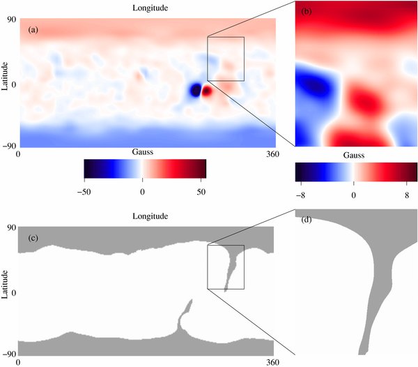
Figure 1. (a) Radial component of the magnetic field (Br) from a smoothed NSO Kitt Peak map for Carrington rotation (CR) 1913 (1996 August 22–September 18). (b) Enlargement of (a). (c) Open/closed-field boundaries (coronal hole map) for an MHD model of the solar corona using the flux distribution of (a) as a boundary condition. (d) Enlargement of the coronal hole map showing the elephant's trunk (southward extension of the northern coronal hole).
Download figure:
Standard image High-resolution imageTo study the effects of small-scale parasitic (opposite) polarities, we add two small artificial bipoles in the area around the elephant's trunk (shown as an enlargement in Figure 1(b)), creating the magnetic flux distribution shown in Figures 2(a) and (b). We stress that this new flux distribution is not meant to match any particular observation during this time period, but to test the ideas outlined in the introduction. We initiate a new simulation with this flux distribution in the same way described above, relaxing the configuration for a period of about 56 hr. The coronal hole map for this configuration is shown in Figures 2(c) and (d). As it is evident from Figure 2(c) and especially from the enlargement in Figure 2(d), introducing these bipoles causes a "break up" of the elephant's trunk coronal hole and inserts some closed flux in areas that were originally open. After the relaxation period, we introduced a surface flow that is uniform in longitude and directed from west to east, vϕ0 ≈ −1 km s-1 between 305 ≲ Lat. ≲ 360, and between 78 ≲ Lat. ≲ 153. This flow does not represent an actual observed flow on the Sun; it is used as a convenient way of moving open and closed flux associated with the bipoles into the streamer belt region. After 70 hr, the flow was stopped and we allowed the system to relax further for 14 hr. We used this flow (as opposed to an observed flow, like differential rotation) so that the bipoles would be advected away from the coronal hole and into the closed-field region more rapidly, shortening the computation time. We have found that for simulations like this one, the magnitude of the flow does not affect the results, as long as it is much less than the ambient Alfvén speed.

Figure 2. (a) Initial Br distribution for the simulation, consisting of the magnetic map of Figure 1(a) with two small bipoles introduced into the region occupied by the elephant's trunk. (b) Enlargement showing the magnetic flux distribution around the bipoles. (c) Coronal hole map calculated with the MHD model for the Br distribution shown in (a). (d) Enlargement of the elephant's trunk, showing that some open flux in the configuration of Figure 1 is now closed.
Download figure:
Standard image High-resolution image3. RESULTS
The velocity flow we apply to advect the bipoles is uniform in longitude and, consequently, its effects are felt in the global corona. Figure 3 shows a sequence of surface magnetic flux maps with the coronal hole maps superimposed at different stages of the simulation. Time in hours is indicated in the figure; t = 0 is taken to be the end of the relaxation phase when the flows are introduced. Shaded areas represent open-field regions. This arrangement can be compared with Figures 1 and 2, where the magnetic flux and coronal hole maps are shown separately. From the global evolution (left column) sequence, it can be seen that the shearing flow causes the northern and southern coronal holes to grow. This occurs because the large-scale field is energized by the flows and the closed-field loops rise in response. The outermost of these closed loops are then susceptible to being carried out by the solar wind and the open-field regions increase in size.

Figure 3. Evolution of Br and coronal hole boundaries when surface flows are introduced into the simulation. The coronal hole map has been superimposed on the map of Br, so that open flux regions are shaded. t = 0 corresponds to the end of the initial relaxation when the flows are introduced. The left column shows the global evolution, the right column an enlargement centered around the elephant's trunk coronal hole. The location and direction of the imposed longitudinal flow vϕ0 is indicated in the rightmost frame at 42 hr. A further enlargement of the areas surrounding the bipoles (the green and blue rectangles) is presented in Figures 4 and 7.
Download figure:
Standard image High-resolution imageThe right column of Figure 3 shows an enlargement of the area surrounding the elephant's trunk coronal hole. The introduction of the two bipoles affects the structure of the coronal hole, causing closed magnetic field to appear within the elephant's trunk, where the field would have been completely open otherwise. The coronal hole is associated with field of positive polarity and magnetic field lines of positive sign, instead of opening up to space, close down in the negative polarity portions of the two bipoles. We refer to the two bipoles as northern and southern; the areas surrounding the northern bipole and southern bipole are colored respectively in green and blue rectangles. The evolution of these areas is shown enlarged in the sequences in Figures 4 and 7, which again present a superposition of magnetic flux maps with coronal hole maps.

Figure 4. Closeup of the evolution in the region surrounding the northern bipole (green rectangles in the right column of Figure 3). Open flux regions are shaded, as in Figure 3. As the positive polarity of the bipole is advected into the closed-field region, the open flux associated with it closes down.
Download figure:
Standard image High-resolution image3.1. Evolution Associated with the Northern Bipole
Figure 4 depicts the evolution of the northern bipole as it is advected eastward (from right to left in the figure) by the surface flow. In the early phases of the evolution, open flux closes down and new open flux is formed via interchange reconnection. As the evolution proceeds, the closed-field region surrounding the negative polarity merges with the eastern closed flux area. Eventually, the open flux associated with the positive polarity enters the closed-field region and, as can be seen by the coronal hole map, does not remain open but closes down. A weaker negative polarity, associated with closed flux, trails behind the positive polarity and eventually merges with the closed field on the left. The process whereby open flux closes down is shown in Figure 5, which presents a three-dimensional perspective of the advection of the northern bipole. Open-field lines traced from the positive polarity of the bipole are shown in green. As can be seen in the figure, as the positive polarity spot enters the closed-field region, reconnection begins to close down the flux. Eventually all the flux associated with the positive polarity reconnects and no open flux is left.

Figure 5. Magnetic field lines in a three-dimensional view of the evolution shown in Figure 3 and 4. Open fields emanating from the positive polarity of the northern bipole are shown in green. Br and coronal hole boundaries are shown on the solar surface. Eventually all the flux associated with the positive polarity reconnects and closes down. A view from further distance for the same times is portrayed in Figure 6.
Download figure:
Standard image High-resolution image
Figure 6. Evolution of the magnetic flux in normalized units. Field lines have been traced from 10 R☉ to track the behavior of the magnetic flux. Folded flux is associated with field lines with a polarity inversion in the radial component of the magnetic field and is a proxy for flux that has undergone interchange reconnection. Disconnected flux is associated with field lines with both ends at the outer radial boundary. Interchange reconnected and disconnected flux are a tiny fraction of the open flux (3–4 orders of magnitude difference) in the simulation. The (a)–(d) frames of Figure 5 are also shown, viewed from a position more distant from the Sun. The solar surface is shaded with the coronal hole map (black regions are open). Magnetic reconnection occurs at the HCS above the helmet streamer and at the null point associated with the parasitic polarity region of the bipole. During the closing down of the bipolar flux, the disconnected flux peaks in frames (b) and (c).
Download figure:
Standard image High-resolution imageIt should be emphasized that in our simulation, as in the real Sun, there are at least two sites for reconnection. One is at the null and separatrix surface associated with the embedded bipole. As described in Edmondson et al. (2010) the reconnection here is primarily of the interchange type. Closed–closed reconnection does occur while the bipole is moving purely through the closed-field region, but this has minimal effect on the open field. The other site of reconnection, which was not included in Edmondson et al. (2010), is at the HCS. This reconnection has important heliosperic signatures because it can produce disconnected flux in the wind.
To further investigate the structural changes that occur in the magnetic field during the evolution, we tracked magnetic flux in the simulation by tracing magnetic field lines in both directions from r = 10 R☉. We classified field lines according to their structure in the following manner. Field lines are considered to be open if one end connects to the surface of the Sun and the other reaches the outer boundary of the simulation. Closed-field lines have both ends connected to the solar surface. Disconnected flux is defined as flux associated with field lines with both endpoints on the outer radial boundary. We identified interchange reconnection by the presence of folded flux, field lines that are open but Br changes sign in the simulation domain. This fold in the field line naturally occurs as part of the interchange reconnection process, as seen in the depiction by Crooker et al. (2002) and in the simulations of Lionello et al. (2005; see Figure 4(c)). We traced as many as 16 million field lines in each time slice to track these different structures. Nevertheless, our identifications can only be regarded as approximate because of the vast region of the simulations, and the presence of nulls, separators, and QSLs. As the interchange reconnection occurs primarily at the null points associated with the small bipoles, our calculation of interchange reconnected flux is likely to be a lower limit to the actual amount (see Section 3.2).
Figure 6 shows the evolution of the unsigned magnetic flux for the different categories during the bipole advection phase. Also shown is a view of the magnetic field lines depicted in Figure 5, but viewed from a further distance and with a coronal hole map depicted on the surface. As we trace field lines from 10 R☉, we do not account for most of the closed flux in the simulation, which actually dominates (closed flux does not typically rise above r = 3–4 R☉ in the steady-state solution). Measured in this way, open flux forms the bulk of the total flux, followed by the closed flux (almost 2 orders of magnitude less), and folded and disconnected flux (3–4 orders of magnitude less). As noted earlier, the introduction of uniform flows energizes the entire corona and leads to a general pattern of closed flux being opened during the advection phase. The evolution of the closed flux at 10 R☉ can be understood as follows: upper field lines of closed flux tend to rise and be caught up by the solar wind in the early phase of the advection. As the apex of these closed-field lines pass 10 R☉, the amount of closed flux increases. This increase is only temporary. As the field lines continue to rise, the apex of the loops leaves the simulation domain and the flux is categorized as open, decreasing the amount of closed flux and increasing the open flux. This pattern tends to repeat as different portions of closed flux become energized and transition to open flux.
In the initial evolution after the flows are introduced, some interchange reconnection appears but no evidence for disconnection is found. The largest amount of disconnected flux appears during the closing down of the northern dipole between t = 34 and t = 39 hr. The magnetic reconnection that closes down the open bipole occurs primarily by reconnection across the HCS. We did not find any evidence for open magnetic flux being transported into the closed-field regions, as required by the interchange model. This result is contrary to the requirements of the mechanism envisioned by Fisk & Schwadron (2001) to explain the polarity inversion of the Sun during its 11 year cycle. The formation of reconnected flux is in contradiction with the results of Crooker et al. (2002), who argued that disconnected flux must be very rare because heat flux dropouts, which are associated with magnetic field lines that are not connected to the Sun, are hardly observed. However, Owens & Crooker (2007) showed that electron dropouts would be very difficult to observe even if disconnected flux were responsible for restoring the flux balance in response to ICMEs. Hence, disconnection of flux cannot be ruled out through current empirical evidence.
We must emphasize that a particular case has been simulated here, and the relative amounts of interchange reconnection and disconnection may be different if finer scale structure is included in the photospheric field, and more general motions applied. However, disconnection (as well as interchange reconnection) also occurred in the vicinity of the HCS in the simulations of Lionello et al. (2005, 2006), where the effects of differential rotation were studied. Evidently, it is difficult to avoid some disconnection when photospheric magnetic flux is advected. In retrospect, this should not be surprising. The HCS is an obvious place in the corona for opposite polarity fields to come in contact. Advection of flux will not always result in opposite polarity open field always finding a closed field to reconnect with—sometimes it will find another open-field line, and disconnect. We note from Figure 6 that both the disconnected flux and the interchange reconnected flux were orders of magnitude lower than the total open flux in the simulation. Nevertheless, based on our simulations we would predict that disconnected flux should be occasionally present near the HCS.
3.2. Evolution Associated with the Southern Bipole
We now discuss the evolution of the southern bipole in the simulation, shown in Figure 7. In this case, the negative polarity portion of the bipole almost splits the extended coronal hole into two pieces. However, in agreement with the Antiochos conjecture, the two portions of the coronal hole are connected by a narrow corridor of open flux on the eastward side of the bipole. As the bipole is advected eastward, this corridor reforms on the westward side of the bipole, and the coronal hole is stretched by the advection of the positive polarity portion of the bipole.
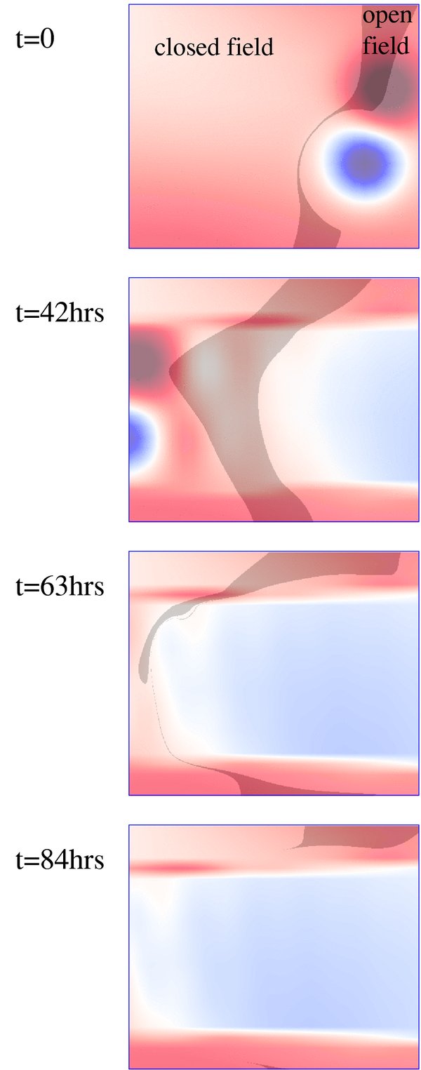
Figure 7. Closeup of the evolution in the region surrounding the southern bipole (blue rectangles in the right column of Figure 3). When the large region of negative polarity field is advected into the extended coronal hole, the hole appears to be split into two pieces, forming an apparently isolated coronal hole.
Download figure:
Standard image High-resolution imageA serendipitous result was obtained as the simulation continued. A large negative polarity region westward of the coronal hole was advected eastward and protruded into the positive polarity of the coronal hole (light blue region in the center of the t = 63 hr and t = 84 hr frames of Figure 7). This negative polarity (associated with the synoptic map for this time period, and not due to the introduced bipole) splits off and isolates a region of positive polarity of the elephant's trunk coronal hole. This is also evident in Figure 3. The coronal hole itself has also seemingly broken into two separate coronal holes. This is most easily seen in Figure 8(a), which shows both the photospheric neutral lines and the coronal hole boundaries. Examination of Br above 3 R☉ shows that there is still a single HCS in the configuration. As discussed in the introduction, a truly isolated coronal hole under these circumstances would be in contradiction with the Antiochos conjecture. According to the conjecture, an isolated coronal hole must in fact be connected by a very narrow corridor of open flux. Does such a corridor connect the two apparently separate coronal holes?
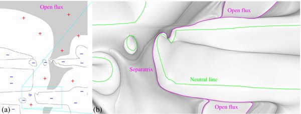
Figure 8. Two maps showing the magnetic field topology at the end of the simulation. (a) A coronal hole map with neutral lines. Shaded areas indicate open field. Within a single same polarity region, there seem to be two separate coronal holes, which have originated from the breaking-up of the single coronal hole present at the beginning of the simulation. (b) An enlargement showing a log Q (defined in Section 3) map of the area in the cyan box. Neutral lines are in green. The two coronal holes are actually linked through a zero-width separatrix line.
Download figure:
Standard image High-resolution imageTo investigate this question, we traced field lines in the area between the two open-field regions in Figure 8(a) at increasingly higher resolution. We could not find any evidence of a finite open-flux corridor at the photosphere. To study the topology more systematically, we computed the "squashing" factor Q (Titov 2007), which measures the elliptical deformation of the cross section of an infinitesimal flux tube. It is very useful for identifying important features of the magnetic field. High values of Q result from topological features such as null points, separatrix surfaces, and separator field lines, as well as geometrical features such as QSLs. Figure 8(b) shows a map of the Q factor on a logarithmic scale for an enlargement of the region outlined in the cyan rectangle in Figure 8(a).
The locally highest values of Q are highlighted in magenta in the figure. As expected, Q is particularly large at the boundary of the coronal holes, since a true separatrix surface exists here that divides the topologically distinct areas of open and closed flux. Q ought to be infinite under these circumstances, but obtains a finite value when computed on a grid. A line of very large Q also connects the two open flux regions. We have found that this line also behaves like a discontinuity in field connectivity. Field lines traced from the photosphere in the neighborhood of this line always divert to one side or the other with end points far away from one another.
It is difficult to demonstrate conclusively that a structure is a true discontinuity in a calculation on a finite grid. To analyze this result more rigorously, Titov et al. (2011) developed an exact analytic source-surface model that closely resembles the configuration in this simulation. They show that in these circumstances a zero-width footprint of a separatrix dome, rather than a finite corridor, is present at the boundary of the calculation. Therefore, we refer to the line of large Q linking the coronal holes as a separatrix footprint. Formally, our detached coronal hole violates the Antiochos conjecture in its original form, because no finite corridor exists between the two coronal holes at the photosphere. (A finite corridor would correspond to the footprint of a QSL.) However, as discussed by Titov et al. (2011), the essential nature of the conjecture is preserved if we modify it to state that coronal holes within the same polarity always remain linked, either by a finite-width corridor or a zero-width separatrix footprint. It is the linking of apparently disconnected coronal holes to the polar coronal hole (whether by separators or corridors) that is physically significant because it implies that coronal hole boundaries are not smooth but have a complex structure.
In practice, the physical difference between QSLs and true separatrix surfaces may not be very important. Both are regions where electric current concentrations would be expected to form when the footpoints of the fields are stressed, and sites where the magnetic field is most susceptible to reconnection. We have found large current densities in the vicinity of regions where Q is large, but the present calculation has insufficient resolution to carefully investigate reconnection in these regions. Investigation of reconnection in this context will be the subject of future work. We note that while no finite-width corridor forms at the photosphere, a thin corridor does appear at very low heights in the corona, as demonstrated in Figure 9. Coronal hole maps developed by tracing at four heights in the calculation are shown in the figure. The map at the solar surface (Figure 9(a)) shows no open-field lines at the separator. At about 21,000 km above the surface (1.032 R☉; Figure 9(b)), a narrow corridor of open field can be found in the corona near the separatrix footprint. This corridor of open flux widens rapidly (Figures 9(c) and (d)) with increasing height. While it is not surprising that the field expands from a thin coronal hole, the novel result here is that a relatively simple photospheric flux distribution leads to exotic topologies involving singular links between coronal holes at the photosphere and multiple null points appearing in the corona. This is discussed in detail by Titov et al. (2011).

Figure 9. Four coronal hole maps at different heights in the calculation, zoomed in on the region where a separator links the seemingly isolated coronal hole to the southern extension of the polar coronal hole. (a) Map at r = R☉ (lower boundary of the calculation). Field lines traced from the lower boundary do not open in the vicinity of the separator. They remain closed and divert to one side of the separator or the other. (b) Map at r = 1.032 R☉. This is the lowest height at which we can conclusively demonstrate open-field lines by tracing near the separator. The coronal holes are now connected by a narrow corridor. When these field lines are traced back to the lower boundary, they map back to either the southern extension of the coronal hole or the lower, linked coronal hole. (c) Map at r = 1.038 R☉ (about 2 grid points above the map in (b)). The corridor of open field thickens rapidly. (d) Map at r = 1.05 R☉. The corridor has grown to the point that it is nearly as wide as the linked coronal holes.
Download figure:
Standard image High-resolution image
The presence of separatrix surfaces and QSLs in the simulation domain implies that it is numerically challenging to identify structural features in the magnetic field via field line tracing, as was done in Figure 6. In constructing this figure, as we increased the number of tracing points, the amount of flux identified as disconnected or interchange reconnected (really folded flux) rose slightly compared to the open and closed flux (which did not change). We must also allow for the possibility that some flux that interchange reconnects at the null point of the bipole will produce a field line with a change in curvature but not a second minima in radius (and thus not be identified as folded). Therefore, the percentage of disconnected/interchange reconnected flux relative to open flux identified in Figure 6 must be regarded as approximate, and a lower limit to the amount present.
3.3. Implications for the Interchange Model and the Origin of the Slow Solar Wind
Our results shown in Section 3.1 show that we cannot easily advect open magnetic flux into closed-field regions. The flux tends to close down, accompanied by some disconnection. This result conflicts with the requirements of the interchange model, which proposes that open magnetic flux is transported by interchange reconnection from one pole to the other during the course of the solar cycle and the reversal of the polar fields. An important aspect of the interchange model is that it predicts that interchange reconnection is the predominant source of the slow wind, thus accounting for its elemental composition and freeze-in temperatures. Our results show that both QSLs and separatrix surfaces can form as a result of the surface motions of photospheric magnetic flux. Separatrix surfaces and QSLs are the sites where interchange reconnection is most likely to occur. Therefore, our results support this facet of the interchange model. Antiochos et al. (2011) describe the identification of QSLs and separators in a high-resolution model of the solar corona for the time period of the 2008 August 1 solar eclipse and, in a new hypothesis dubbed the S-web model, propose that interchange reconnection at these sites may be an important source for the slow solar wind. Subramanian et al. (2010) show evidence for intermittent reconnection near the boundaries of coronal holes, and argue that outflows associated with these events could be a source of the slow wind.
4. CONCLUSIONS
We have used our three-dimensional MHD model to investigate two conflicting concepts that have arisen as part of the debate on the structure and evolution of open magnetic flux in the corona and heliosphere. (1) The idea that open flux can diffuse into the streamer belt and remains open (from the interchange model); (2) isolated coronal holes are in actuality always connected (possibly by extremely narrow corridors) to the polar coronal hole of the same polarity (the Antiochos conjecture). Our results can be summarized as follows.
- 1.Open flux associated with the northern bipole did not remain open when it was advected into the closed-field region. This conflicts with the requirements of the interchange model.
- 2.While interchange reconnection did indeed occur during the simulation, both opening and disconnection also occurred, in conflict with the interchange model. From this simulation and the previous results from Lionello et al. (2005, 2006), it appears to be difficult to avoid some disconnection when photospheric motions move the footpoints of magnetic flux that lies near the HCS. This is generally a very small percentage of the total open flux in the simulations (see Figure 6). Therefore, we would predict that disconnected flux should appear occasionally in the vicinity of the HCS. As discussed by Owens & Crooker (2007), the most obvious signature of disconnected flux, heat flux dropouts, would be rarely observed by spacecraft at 1 AU even if disconnected flux was present. Crooker & Pagel (2008) reexamined Wind data and concluded that interchange reconnection and disconnection could not be distinguished from one another in the electron data. The proposed Solar Probe Plus mission, which will make in situ observations much closer to the Sun, may be able to confirm or refute this prediction.
- 3.The introduction of the southern bipole causes the lowest part of the elephant's trunk coronal hole to be nearly detached, but it remained connected through a narrow corridor of open flux, in agreement with the Antiochos conjecture (Antiochos et al. 2007). In the early evolution of the simulation, this narrow corridor was maintained, but eventually detaches when a large region of negative polarity flux intrudes and splits the positive polarity of the extended coronal hole. By plotting a map of Q, we find that these two coronal holes are linked at the photosphere by a line of very large Q. Subsequently, Titov et al. (2011) have shown that this line is in fact a zero-width footprint of a separatrix dome. A narrow corridor of open field forms between the coronal holes at a low height (1.032 R☉).
- 4.As discussed by Titov et al. (2011), the main result of the Antiochos conjecture holds if we modify it to state that coronal holes of the same polarity are always linked, either by finite width corridors or zero-width separatrix footprints.
- 5.While our results are in disagreement with some important aspects of the interchange model in its present form, the discovery of separator formation indicates that the boundary of coronal holes is not likely to be smooth, but in fact may exhibit a rich structure where opposite polarity open and closed fields may be in close proximity. Therefore, our results actually provide support to a primary inference of the interchange model: interchange reconnection may be an important source for the slow solar wind. This aspect of our results are discussed in more detail by Antiochos et al. (2011).
- 6.Addressing whether interchange reconnection at separators and QSLs can supply the slow solar wind plasma ultimately requires very high resolution simulations of realistic coronal fields with random-footpoint motions imposed. Such simulations are extremely challenging, but may be possible in the next few years.
This work was supported by NASA's Heliophysics Theory, LWS, and Guest Investigator programs, the LWS Strategic Capabilities Program (NASA, NSF, and AFOSR), and the Center for Integrated Space Weather Modeling (an NSF Science and Technology Center). Computational resources were provided by the NSF supported Texas Advanced Computing Center (TACC) in Austin and the NASA Advanced Supercomputing Division (NAS) at Ames Research Center. This work was initiated and greatly benefitted from discussions in the LWS TR&T focus team on the solar and heliospheric magnetic field.