


ABSTRACT
We present the results of a Jupiter Trojans' light curve survey aimed at characterizing the rotational properties of Trojans in the approximate size range 60–150 km. The survey, which was designed to provide reliable and unbiased estimates of rotation periods and amplitudes, resulted in light curves for a total of 80 objects, 56 of which represent the first determinations published to date and nine of which supersede previously published erroneous values. Our results more than double the size of the existing database of rotational properties of Jovian Trojans in the selected size range. The analysis of the distributions of the rotation periods and light curve amplitudes is the subject of companion papers.
Export citation and abstract BibTeX RIS
1. INTRODUCTION
Jovian Trojan asteroids are a population of objects co-orbital with Jupiter. Because of their greater distance and consequent fainter apparent magnitudes, these objects have been generally less frequently observed than main belt asteroids.
There are two groups of Jovian Trojans, each consisting of objects that librate about the Lagrangian equilateral stability points L4 and L5 of the Sun–Jupiter system, respectively, leading and trailing Jupiter by 60° in heliocentric ecliptic longitude. These objects have been demonstrated to be dynamically stable over the age of the solar system (Levison et al. 1997).
Because of their special location, Trojans are of particular interest and importance for understanding the origin and evolution of Jupiter and its system of inner (regular) and outer (irregular) satellites. The surface and internal compositions of the Trojans are expected to reflect the materials and conditions in the solar nebula at the time and location of their accretion.
As of 2010 August 20, there were 2800 known asteroids in the L4 group and 1757 in the L5 group.10
From a wide-field photographic survey centered on the leading Trojan cloud, and covering about 700 deg2, Lagerkvist et al. (2000) estimated a population of about 1100 L4 Trojans down to a size of 17 km. By analyzing the serendipitous discoveries of Trojans during a trans-Neptunian object survey covering about 20 deg2 Jewitt et al. (2000) estimated an L4 population of ∼1.6 × 10⁵ down to a diameter of 2 km, with a combined mass of ∼10−4 Earth masses. The mean collision velocity in the Trojan clouds is about 5 km s−1, similar to that in the main belt (Marzari et al. 1997; Dell'Oro et al. 1998, 2001). This similarity is due to the lower Keplerian velocities at the heliocentric distance of the Trojan clouds being compensated by the higher average orbital inclinations of the Trojans. The intrinsic collision probability for the Trojans is about twice that found in the main belt (Dell'Oro & Paolicchi 1998; Dell'Oro et al. 1998), which, contrary to what was commonly accepted earlier, leads to a picture of a Trojan population where considerable collisional evolution takes place. This scenario is further confirmed by the discovery of dynamical families among the Trojans (Milani 1993).
Shape and angular momentum are acquired during the accretion process, and are affected by the subsequent collisional evolution of the bodies. The characterization of these properties can provide important clues to the history of the Trojans. Light curve observations represent the basic tool for determining the rotational properties of asteroids, allowing for the determination of the rotation rate, rotational axis direction, and an estimate of the body shape. Some important physical properties, directly related to the outcome of collisional events, can be inferred from light curve observations.
Early work by Hartmann et al. (1988), Zappalà et al. (1989), and Binzel & Sauter (1992), the latter being based on a sample of 31 objects, suggested that Trojans might have a larger incidence of high-amplitude light curves, compared to main belt asteroids. Based on these data, the authors proposed that these objects may possess considerably elongated shapes, possibly reflecting a difference in composition and/or collisional evolution with respect to their counterparts in the main belt. In particular, Hartmann & Tholen (1990) proposed a similarity between Trojans and cometary nuclei, and hypothesized a mechanism of topography exaggeration by sublimation of volatiles, which could explain the elongated shapes of Trojans.
These initial investigations, however, were based on a limited sample and were affected by an observational bias tending to favor the determination of high amplitudes and short periods.
More recently, Mann et al. (2007) conducted a sparse-sampling photometric survey to perform a statistical investigation of the light curve amplitudes of Jovian Trojans which was designed to detect possible large-amplitude contact binary candidates. In their work, the authors acquired five exposures for each object, for a total of 114 Trojans. Due to its own nature, however, the survey could only provide lower bounds for the amplitudes and produced period determinations for only two objects.
The necessity of determining a sizable, reliable, and unbiased sample of rotation periods and amplitudes has motivated our observational program to systematically explore the rotational properties of Trojans. For this reason we mostly selected targets brighter than an absolute magnitude H = 10 (or a diameter of about 60 km) and aimed at achieving a good degree of completeness down to this limit. The fact that the survey has been performed under uniform conditions also makes it easier to assess possible bias sources.
This paper reports the results of the light curve observations for 80 objects acquired in the course of this program over two decades. The analysis of the distributions of the rotation periods and light curve amplitudes is the subject of companion papers. Preliminary results from an earlier stage of this survey were also summarized in Barucci et al. (2002).
2. OBSERVATIONS
In order to determine the rotational properties of the target objects, we performed time-resolved CCD photometric series in the optical range. We used the technique of differential photometry, which makes use of field stars present in the same CCD frame as the target to allow for accurate removal of atmospheric extinction variability. Depending on the spectral sensitivity of the particular CCD used and on the instrumental setup, the observations were performed in the V and/or in the R spectral bands, aiming to maximize the signal-to-noise ratio (S/N) of the measurements.
The telescope was generally unguided, and tracked halfway between the rate of the object and the sidereal rate, in order to produce a similarly shaped point-spread function for both the target and the reference stars. The telescope fields were carefully centered to keep suitable reference stars within the CCD frame for the whole night.
The exposure times were chosen to produce an S/N between 80 and 150, which typically resulted in exposures between 1 and 5 minutes, the upper limit being determined by cosmic hits contamination and telescope guide errors. As no super-fast rotation is possible in the size range of the observed objects for any realistic material strength, even the longest exposures provide adequate sampling for any possible rotation period.
In general, whenever the telescope provided reliable pointing, we cycled between three and six objects per night, aiming to obtain an approximately uniform sampling at a rate of one data point every 15–30 minutes and the longest possible baseline. Whenever possible, the objects were then re-observed on subsequent nights, until a reliable period could be determined.
During nights of photometric quality, we acquired calibration sequences of the target objects and of photometric standard stars in the V band, in order to tie the observed magnitudes to the Johnson standard system. In addition to the Landolt Catalog (Landolt 1983), we used stars from the Guide Star Photometric Catalog (GSPC; Lasker et al. 1988) as photometric standards. Although the latter contains only tertiary standard stars, its advantage is a high density of stars throughout the celestial sphere, in a range of brightness well suited to CCD photometry. The use of the GSPC enabled us to select standard stars with solar-like colors located within only a few degrees of the target objects. As a consequence, these star fields were observed (generally close to their culmination) at air masses very close to those of the target objects, thereby minimizing the contribution of the error in the extinction coefficient on the determination of the absolute magnitude. Further, the similarity of the colors of the targets and of the standard stars made a color index correction unnecessary. The resulting accuracy of the absolute calibrations was typically in the range of 0.02–0.03 mag rms.
The observations were carried out using a number of different telescope and instrument combinations as detailed in Table 1.
Table 1. Telescopes and Instruments
| Telescope | Instrument | Detector | Plate Scale (arcsec pixel−1) | Field of View (arcmin) | |
|---|---|---|---|---|---|
| 1 | ESO, 61 cm Bochum | DLR MKII | Tek 1024 × 1024 | 0.54 | 9.2 × 9.2 |
| 2 | ESO, 90 cm Dutch | CCD Camera 29 | Tek 512 × 512 | 0.46 | 3.9 × 3.9 |
| 3 | ESO, 1 m | DLR MKI | Thomson 384 × 576 | 0.35 | 2.2 × 3.4 |
| 3 | ESO, 1 m | DLR MKI + focal red. | Thomson 384 × 576 | 0.54 | 3.5 × 5.2 |
| 4 | ESO, 1 m | DLR MKII | Tek 1024 × 1024 | 0.30 | 5.2 × 5.2 |
| 5 | Calar Alto, 1.2 m | CCD Camera 2b 17 | SITe 2048 × 2048 | 0.46 | 15.8 × 15.8 |
| 6 | Pino Torinese 1 m | SCAM-2 | Loral 2048 × 2048 | 0.31 | 10.6 × 10.6 |
| 7 | Loiano 1.52 m | DLR MKI | Thomson 384 × 576 | 0.50 | 3.2 × 4.8 |
| 7 | Loiano 1.52 m | DLR MKI + focal red. | Thomson 384 × 576 | 0.77 | 5.0 × 7.4 |
| 8 | Loiano 1.52 m | BFOSC | e2v 1340 × 1300 | 0.58 | 12.6 × 13.0 |
| 9 | Kvistaberg 100/135 cm | DLR MKII | Tek 1024 × 1024 | 0.41 | 7.0 × 7.0 |
| 10 | OAVdA 81 cm | FLI ProLine | Fairchild 2048 × 2048 | 0.97 | 16.5 × 16.5 |
Download table as: ASCIITypeset image
3. DATA REDUCTION
The reduction of the CCD frames consisted of conventional dark removal and flat-fielding, which was performed by using high S/N dark and flat calibration frames. The flat fields were acquired by observing dithered sky fields during twilight and subsequently removing the field stars. Care was taken to use exposure times that were long enough that the shutter-induced exposure non-uniformity stayed below 0.5% from center to edge. Morning and evening flats were also compared to expose possible straylight contamination.
The source flux extraction was performed with AstPhot, a synthetic photometric aperture application developed at DLR (Mottola et al. 1995). Within AstPhot, the user interactively selects the comparison stars and the target object to be measured and defines the size and the shape of the synthetic apertures to be used (parameterized as an ellipse) and the regions to be used for the background estimation. In a case where the synthetic aperture of the target is different from those of the comparison stars (e.g., due to the adopted tracking rate), an aperture correction factor is introduced based on a photometric growth curve analysis. Typical aperture sizes used for these observations range from 5'' to 10''. The comparison stars were checked against each other to detect possible variability, and were then used to determine the atmospheric extinction. The resulting observed magnitudes (relative to the comparison stars, or, if calibrations were available, expressed in the Johnson system) were then reduced to unit distance from Earth and from the Sun. Furthermore, the times of the observations were light-travel subtracted, and a small correction for compensating the varying solar phase angle during the night applied, following the HG system.
The individual-night light curves were then merged into a composite by using the Fourier analysis procedure described in Harris et al. (1989). In this method, a light curve is approximated with a Fourier polynomial of the desired order. For each trial rotation period within a given range, a linear equation system is constructed, which is then least-squares fitted to the data to retrieve the best-fit Fourier coefficients and an individual night's magnitude shifts. A solution is achieved if a global minimum of the residuals in the chi-squared sense is found, under the assumption that the number of light curve extrema per cycle (usually, but not necessarily, two maxima and two minima) is known. One of the critical issues about the period determination is the presence of possible alias solutions, which can arise from a combination of causes such as inadequate sampling, incomplete coverage, commensurabilities with the Earth day length and light curves with an unusual number of extrema. A careful design of the observations helped us reduce some of these effects.
The possibility of having a quick-look data reduction capability at the telescope proved to be key to the success of the observations. In this way, it was possible to schedule the next night's observations in an efficient way by securing full coverage of the light curve, avoiding repetitions, and adjusting the exposure times, if necessary.
Table 2 reports the observational circumstances for the target objects. The date of observation is given to the tenth of the day closest to the mid-time of the observations. The following columns report the ecliptic longitude and latitude, the solar phase angle, the geocentric and heliocentric distances, the V magnitude reduced to 1 AU, the telescope and instrument combinations, and the observers, respectively.
Table 2. Observational Circumstances and Mean Magnitudes
| Asteroid | UT Date | λ | β | α | r | Δ | V(1, α) | Telescope and | Observer | |
|---|---|---|---|---|---|---|---|---|---|---|
| (deg J2000) | (deg) | (AU) | (AU) | Instrumenta | ||||||
| 588 Achilles | 1994 Jul | 3.3 | 288.1 | –6.2 | 1.6 | 5.8958 | 4.8903 | 8.64 | 1 | Mottola |
| 4.3 | 288.0 | –6.2 | 1.6 | 5.8954 | 4.8882 | 1 | Mottola | |||
| 659 Nestor | 1995 Aug | 19.2 | 305.5 | –3.8 | 4.4 | 4.6546 | 3.6931 | 9.02 | 1 | Mottola, Schober |
| 20.2 | 305.4 | –3.7 | 4.6 | 4.6542 | 3.6989 | 1 | Mottola, Schober | |||
| 21.2 | 305.3 | –3.7 | 4.8 | 4.6539 | 3.7038 | 1 | Mottola, Schober | |||
| 22.2 | 305.1 | –3.7 | 5.0 | 4.6536 | 3.7098 | 1 | Mottola, Schober | |||
| 884 Priamus | 1993 Jan | 14.9 | 115.8 | 1.1 | 0.3 | 5.7227 | 4.7393 | 9 | Mottola, Lagerkvist | |
| 18.1 | 115.4 | 1.1 | 0.5 | 5.7216 | 4.7387 | 9 | Mottola, Lagerkvist | |||
| 19.9 | 115.2 | 1.1 | 0.8 | 5.7210 | 4.7399 | 9 | Mottola, Lagerkvist | |||
| 2001 Oct | 16.9 | 46.9 | 10.5 | 4.5 | 5.4862 | 4.5689 | 6 | Delbò, Mottola | ||
| 17.9 | 46.8 | 10.5 | 4.3 | 5.4869 | 4.5638 | 6 | Delbò, Mottola | |||
| 911 Agamemnon | 1997 Nov | 3.9 | 41.9 | 24.6 | 4.8 | 4.8897 | 3.9704 | 6 | Di Martino, Mottola | |
| 18.9 | 39.8 | 24.7 | 5.7 | 4.8879 | 4.0040 | 6 | Di Martino, Mottola | |||
| 23.9 | 39.1 | 24.6 | 6.3 | 4.8874 | 4.0289 | 6 | Di Martino, Mottola | |||
| 1143 Odysseus | 1994 Jun | 3.3 | 293.6 | 3.3 | 6.7 | 5.7253 | 4.9218 | 1 | Mottola | |
| 4.3 | 293.5 | 3.3 | 6.5 | 5.7252 | 4.9114 | 1 | Mottola | |||
| 5.3 | 293.4 | 3.3 | 6.4 | 5.7250 | 4.9012 | 1 | Mottola | |||
| 13.3 | 292.8 | 3.4 | 5.2 | 5.7240 | 4.8280 | 1 | Mottola, Erikson | |||
| 1172 Aneas | 1993 Feb | 27.1 | 122.2 | –17.1 | 6.4 | 5.6776 | 4.8806 | 8.88 | 4 | Mottola, Di Martino |
| 1993 Mar | 1.1 | 122.0 | –17.1 | 6.7 | 5.6772 | 4.8987 | 8.87 | 4 | Mottola, Di Martino | |
| 2.1 | 121.9 | –17.1 | 6.8 | 5.6770 | 4.9081 | 8.89 | 4 | Mottola, Di Martino | ||
| 1437 Diomedes | 1994 Jul | 12.3 | 314.3 | –2.8 | 4.6 | 5.2783 | 4.3378 | 1 | Mottola, Carsenty | |
| 15.3 | 314.0 | –2.7 | 4.1 | 5.2776 | 4.3188 | 1 | Mottola, Carsenty | |||
| 16.3 | 313.9 | –2.6 | 3.9 | 5.2774 | 4.3131 | 1 | Mottola, Carsenty | |||
| 1749 Telamon | 1995 Aug | 19.2 | 298.5 | –4.5 | 4.7 | 5.6729 | 4.7561 | 10.00 | 1 | Mottola, Schober |
| 20.2 | 298.4 | –4.5 | 4.9 | 5.6725 | 4.7631 | 1 | Mottola, Schober | |||
| 21.1 | 298.3 | –4.4 | 5.1 | 5.6720 | 4.7704 | 1 | Mottola, Schober | |||
| 25.1 | 297.9 | –4.4 | 5.7 | 5.6702 | 4.8020 | 10.04 | 1 | Mottola, Schober | ||
| 1867 Deiphobus | 1994 Feb | 8.2 | 136.0 | –18.8 | 3.5 | 5.3240 | 4.3820 | 4 | Mottola, Erikson | |
| 9.2 | 135.9 | –18.9 | 3.5 | 5.3238 | 4.3828 | 8.91 | 4 | Mottola, Erikson | ||
| 10.2 | 135.7 | –18.9 | 3.6 | 5.3236 | 4.3838 | 4 | Mottola, Erikson | |||
| 11.2 | 135.6 | –18.9 | 3.6 | 5.3234 | 4.3852 | 4 | Mottola, Erikson | |||
| 12.2 | 135.4 | –19.0 | 3.7 | 5.3231 | 4.3870 | 4 | Mottola, Erikson | |||
| 17.2 | 134.7 | –19.1 | 4.2 | 5.3221 | 4.3999 | 4 | Mottola, Erikson | |||
| 18.2 | 134.6 | –19.1 | 4.3 | 5.3219 | 4.4034 | 4 | Mottola, Erikson | |||
| 1868 Thersites | 1994 Jun | 7.3 | 299.8 | 19.8 | 8.4 | 5.0776 | 4.3292 | 2 | Mottola, Erikson | |
| 9.3 | 299.7 | 19.8 | 8.2 | 5.0760 | 4.3086 | 2 | Mottola, Erikson | |||
| 10.3 | 290.6 | 19.9 | 8.0 | 5.0752 | 4.2984 | 2 | Mottola, Erikson | |||
| 1873 Agenor | 1994 Feb | 4.2 | 150.0 | –21.4 | 5.0 | 4.9148 | 4.0087 | 10.67 | 4 | Mottola, Erikson |
| 6.2 | 149.8 | –21.4 | 4.8 | 4.9137 | 4.0000 | 4 | Mottola, Erikson | |||
| 7.2 | 149.6 | –21.4 | 4.7 | 4.9132 | 3.9963 | 4 | Mottola, Erikson | |||
| 8.2 | 149.5 | –21.4 | 4.6 | 4.9127 | 3.9928 | 4 | Mottola, Erikson | |||
| 9.2 | 149.3 | –21.4 | 4.5 | 4.9122 | 3.9895 | 10.63 | 4 | Mottola, Erikson | ||
| 2207 Antenor | 1989 Oct | 3.2 | 12.4 | –4.6 | 1.0 | 5.1217 | 4.1244 | 9.20 | 3 | Di Martino, Gonano |
| 4.2 | 12.3 | –4.6 | 0.9 | 5.1216 | 4.1241 | 3 | Di Martino, Gonano | |||
| 5.2 | 12.2 | –4.6 | 0.9 | 5.1214 | 4.1240 | 3 | Di Martino, Gonano | |||
| 9.2 | 11.6 | –4.6 | 1.2 | 5.1209 | 4.1270 | 3 | Di Martino, Gonano | |||
| 1996 Apr | 13.3 | 221.5 | 7.2 | 3.6 | 5.1691 | 4.2113 | 1 | Mottola | ||
| 21.2 | 220.5 | 7.3 | 2.2 | 5.1700 | 4.1814 | 1 | Mottola | |||
| 25.2 | 219.9 | 7.3 | 1.7 | 5.1704 | 4.1734 | 1 | Mottola | |||
| 2223 Sarpedon | 1994 Feb | 8.2 | 171.2 | –16.0 | 6.3 | 5.1805 | 4.3438 | 4 | Mottola, Erikson | |
| 12.2 | 170.7 | –16.1 | 5.7 | 5.1801 | 4.3122 | 4 | Mottola, Erikson | |||
| 16.2 | 170.3 | –16.1 | 5.1 | 5.1797 | 4.2849 | 4 | Mottola, Erikson | |||
| 19.2 | 169.9 | –16.1 | 4.6 | 5.1794 | 4.2673 | 4 | Mottola, Erikson | |||
| 1996 Apr | 11.2 | 237.6 | 3.4 | 6.6 | 5.1086 | 4.2646 | 1 | Mottola | ||
| 15.2 | 237.2 | 3.5 | 6.0 | 5.1083 | 4.2285 | 1 | Mottola | |||
| 20.2 | 236.7 | 3.7 | 5.0 | 5.1080 | 4.1892 | 1 | Mottola | |||
| 24.2 | 236.2 | 3.8 | 4.3 | 5.1078 | 4.1625 | 1 | Mottola | |||
| 2241 Alcathous | 1991 Dec | 13.8 | 69.6 | 5.8 | 2.4 | 5.4299 | 4.4665 | 7 | Mottola, Gonano | |
| 15.8 | 69.3 | 5.7 | 2.7 | 5.4291 | 4.4731 | 7 | Mottola, Gonano | |||
| 17.8 | 69.1 | 5.7 | 3.1 | 5.4283 | 4.4809 | 7 | Mottola, Gonano | |||
| 2260 Neoptolemus | 1995 Aug | 20.2 | 311.5 | –16.5 | 4.2 | 5.1808 | 4.2300 | 1 | Mottola, Schober | |
| 21.2 | 311.4 | –16.5 | 4.4 | 5.1805 | 4.2339 | 10.03 | 1 | Mottola, Schober | ||
| 2002 Mar | 11.9 | 163.8 | 21.4 | 4.1 | 5.2851 | 4.3536 | 8 | Mottola | ||
| 12.9 | 163.6 | 21.4 | 4.2 | 5.2854 | 4.3557 | 8 | Mottola | |||
| 14.1 | 163.4 | 21.3 | 4.3 | 5.2858 | 4.3587 | 8 | Mottola | |||
| 2357 Phereclos | 1994 Feb | 10.2 | 156.7 | –1.4 | 2.9 | 5.1898 | 4.2320 | 4 | Mottola, Erikson | |
| 11.2 | 156.6 | –1.4 | 2.7 | 5.1894 | 4.2274 | 4 | Mottola, Erikson | |||
| 12.3 | 156.5 | –1.4 | 2.5 | 5.1891 | 4.2230 | 4 | Mottola, Erikson | |||
| 14.2 | 156.2 | –1.4 | 2.1 | 5.1884 | 4.2150 | 9.21 | 4 | Mottola, Erikson | ||
| 2010 Jul | 5.0 | 307.9 | 2.7 | 4.9 | 5.0395 | 4.1009 | 5 | Mottola | ||
| 6.0 | 307.8 | 2.7 | 4.7 | 5.0398 | 4.0948 | 5 | Mottola | |||
| 7.1 | 307.7 | 2.7 | 4.5 | 5.0400 | 4.0890 | 5 | Mottola | |||
| 9.1 | 307.4 | 2.7 | 4.1 | 5.0406 | 4.0779 | 5 | Mottola | |||
| 10.1 | 307.3 | 2.7 | 4.0 | 5.0408 | 4.0731 | 5 | Mottola | |||
| 11.1 | 307.2 | 2.7 | 3.7 | 5.0411 | 4.0683 | 5 | Mottola | |||
| 12.1 | 307.1 | 2.7 | 3.5 | 5.0413 | 4.0639 | 5 | Mottola | |||
| 2363 Cebriones | 1994 Feb | 10.2 | 172.6 | –28.9 | 7.3 | 5.1649 | 4.3845 | 4 | Mottola, Erikson | |
| 11.2 | 172.4 | –28.9 | 7.2 | 5.1646 | 4.3769 | 4 | Mottola, Erikson | |||
| 12.2 | 172.3 | –29.0 | 7.1 | 5.1644 | 4.3693 | 4 | Mottola, Erikson | |||
| 13.2 | 172.2 | –29.0 | 7.0 | 5.1641 | 4.3620 | 4 | Mottola, Erikson | |||
| 14.2 | 172.1 | –29.0 | 6.9 | 5.1638 | 4.3549 | 9.51 | 4 | Mottola, Erikson | ||
| 2456 Palamedes | 1995 Aug | 22.2 | 296.2 | –7.3 | 6.0 | 5.3307 | 4.4550 | 1 | Mottola, Schober | |
| 26.1 | 295.8 | –7.1 | 6.6 | 5.3286 | 4.4885 | 9.68 | 1 | Mottola, Schober | ||
| 27.1 | 295.7 | –7.1 | 6.8 | 5.3281 | 4.4975 | 9.64 | 1 | Mottola, Schober | ||
| 28.1 | 295.7 | –7.1 | 6.9 | 5.3276 | 4.5068 | 1 | Mottola, Schober | |||
| 2674 Pandarus | 2001 Oct | 21.9 | 29.7 | –1.1 | 0.3 | 5.5182 | 4.5232 | 8 | Delbò | |
| 2759 Idomeneus | 1991 May | 8.1 | 186.2 | 10.7 | 8.0 | 4.8240 | 4.0271 | 3 | Mottola, Gonano | |
| 10.1 | 186.0 | 10.7 | 8.4 | 4.8244 | 4.0481 | 3 | Mottola, Gonano | |||
| 15.1 | 185.7 | 10.8 | 9.1 | 4.8252 | 4.1024 | 3 | Mottola, Gonano | |||
| 17.0 | 185.6 | 10.8 | 9.4 | 4.8255 | 4.1254 | 3 | Mottola, Gonano | |||
| 1992 Jun | 1.2 | 225.1 | 23.5 | 6.7 | 4.9426 | 4.0724 | 3 | Mottola, Gonano | ||
| 3.1 | 224.9 | 23.4 | 6.9 | 4.9434 | 4.0855 | 3 | Mottola, Gonano | |||
| 4.1 | 224.8 | 23.4 | 7.0 | 4.9438 | 4.0927 | 3 | Mottola, Gonano | |||
| 2010 Nov | 4.1 | 69.1 | –25.2 | 6.5 | 5.2936 | 4.4659 | 5 | Mottola | ||
| 5.1 | 69.0 | –25.2 | 6.3 | 5.2931 | 4.4591 | 5 | Mottola | |||
| 6.2 | 68.9 | –25.3 | 6.2 | 5.2926 | 4.4515 | 5 | Mottola | |||
| 7.0 | 68.8 | –25.3 | 6.1 | 5.2922 | 4.4464 | 5 | Mottola | |||
| 12.0 | 68.1 | –25.5 | 5.6 | 5.2900 | 4.4189 | 5 | Mottola | |||
| 13.1 | 68.0 | –25.6 | 5.5 | 5.2895 | 4.4145 | 5 | Mottola | |||
| 14.1 | 67.9 | –25.6 | 5.4 | 5.2891 | 4.4101 | 5 | Mottola | |||
| 2895 Memnon | 1990 Nov | 15.2 | 75.6 | –30.1 | 6.9 | 4.9575 | 4.1330 | 3b | Mottola | |
| 16.2 | 75.5 | –30.1 | 6.8 | 4.9577 | 4.1280 | 3b | Mottola | |||
| 17.2 | 75.3 | –30.1 | 6.7 | 4.9578 | 4.1233 | 3b | Mottola | |||
| 2920 Automedon | 1994 Jun | 3.2 | 268.8 | 15.1 | 4.1 | 5.2834 | 4.3296 | 1 | Mottola | |
| 4.2 | 268.7 | 15.1 | 4.0 | 5.2833 | 4.3254 | 1 | Mottola | |||
| 10.2 | 267.9 | 15.4 | 3.3 | 5.2829 | 4.3063 | 1 | Mottola, Erikson | |||
| 12.2 | 267.6 | 15.5 | 3.2 | 5.2828 | 4.3022 | 1 | Mottola, Erikson | |||
| 3063 Makhaon | 1994 Jun | 4.3 | 304.9 | 2.1 | 8.4 | 5.4580 | 4.7678 | 1 | Mottola | |
| 5.3 | 304.9 | 2.2 | 8.2 | 5.4581 | 4.7553 | 1 | Mottola | |||
| 6.3 | 304.8 | 2.2 | 8.1 | 5.4582 | 4.7439 | 1 | Mottola | |||
| 2009 Dec | 10.9 | 36.1 | 12.9 | 7.6 | 5.1655 | 4.4140 | 9.16 | 5 | Mottola, Carsenty | |
| 11.9 | 36.0 | 12.9 | 7.8 | 5.1654 | 4.4148 | 9.17 | 5 | Mottola, Carsenty | ||
| 14.8 | 35.8 | 12.7 | 8.2 | 5.1637 | 4.4563 | 10 | Carbognani | |||
| 15.8 | 35.8 | 12.7 | 8.3 | 5.1633 | 4.4673 | 10 | Carbognani | |||
| 16.8 | 35.7 | 12.6 | 8.4 | 5.1628 | 4.4783 | 10 | Carbognani | |||
| 17.8 | 35.7 | 12.6 | 8.5 | 5.1624 | 4.4897 | 10 | Carbognani | |||
| 19.8 | 35.6 | 12.5 | 8.8 | 5.1615 | 4.5134 | 10 | Carbognani | |||
| 3240 Laocoon | 1996 Apr | 16.2 | 204.2 | –2.9 | 0.7 | 5.3563 | 4.3542 | 1 | Mottola | |
| 18.2 | 204.0 | –2.9 | 1.0 | 5.3545 | 4.3537 | 1 | Mottola | |||
| 3317 Paris | 1990 Nov | 12.2 | 79.1 | –29.4 | 6.5 | 5.7191 | 4.9312 | 3b | Mottola | |
| 13.2 | 78.9 | –29.5 | 6.4 | 5.7196 | 4.9250 | 3b | Mottola | |||
| 14.2 | 78.8 | –29.5 | 6.3 | 5.7202 | 4.9191 | 3b | Mottola | |||
| 1998 Jul | 16.0 | 302.8 | 10.2 | 3.1 | 4.5615 | 3.5683 | 5 | Lahulla, Mottola | ||
| 17.0 | 302.7 | 10.1 | 2.9 | 4.5618 | 3.5661 | 5 | Lahulla, Mottola | |||
| 18.0 | 302.5 | 10.1 | 2.7 | 4.5620 | 3.5642 | 5 | Lahulla, Mottola | |||
| 19.0 | 302.4 | 10.0 | 2.6 | 4.5623 | 3.5626 | 5 | Lahulla, Mottola | |||
| 20.0 | 302.2 | 9.9 | 2.5 | 4.5625 | 3.5613 | 5 | Lahulla, Mottola | |||
| 3451 Mentor | 1993 Feb | 27.1 | 119.1 | –23.7 | 7.4 | 5.4368 | 4.6915 | 8.82 | 4 | Mottola, Di Martino |
| 28.1 | 119.0 | –23.7 | 7.5 | 5.4369 | 4.7006 | 8.80 | 4 | Mottola, Di Martino | ||
| 1998 Jul | 16.0 | 290.1 | 29.2 | 6.0 | 4.7480 | 3.8361 | 5 | Lahulla, Mottola | ||
| 17.0 | 289.9 | 29.2 | 6.0 | 4.7478 | 3.8367 | 5 | Lahulla, Mottola | |||
| 18.0 | 289.8 | 29.2 | 6.1 | 4.7476 | 3.8376 | 5 | Lahulla, Mottola | |||
| 19.0 | 289.6 | 29.1 | 6.1 | 4.7474 | 3.8387 | 5 | Lahulla, Mottola | |||
| 20.0 | 289.5 | 29.1 | 6.1 | 4.7472 | 3.8400 | 5 | Lahulla, Mottola | |||
| 3548 Eurybates | 1992 May | 23.2 | 235.4 | –2.2 | 1.3 | 5.5739 | 4.5681 | 9.97 | 3 | Mottola, Gonano |
| 25.3 | 235.1 | –2.3 | 1.7 | 5.5743 | 4.5732 | 3 | Mottola, Gonano | |||
| 26.1 | 235.0 | –2.3 | 1.9 | 5.5744 | 4.5742 | 3 | Mottola, Gonano | |||
| 29.3 | 234.6 | –2.3 | 2.5 | 5.5750 | 4.5853 | 3 | Mottola, Gonano | |||
| 3564 Talthybius | 1994 Jun | 8.3 | 291.6 | –18.4 | 7.0 | 5.1498 | 4.3154 | 1 | Mottola, Erikson | |
| 9.3 | 291.5 | –18.4 | 6.9 | 5.1501 | 4.3075 | 2 | Mottola, Erikson | |||
| 10.3 | 291.4 | –18.4 | 6.8 | 5.1504 | 4.2994 | 2 | Mottola, Erikson | |||
| 11.3 | 291.3 | –18.5 | 6.6 | 5.1507 | 4.2907 | 10.09 | 2 | Mottola, Erikson | ||
| 12.3 | 291.2 | –18.5 | 6.5 | 5.1509 | 4.2849 | 2 | Mottola, Erikson | |||
| 14.3 | 291.0 | –18.6 | 6.2 | 5.1515 | 4.2712 | 2 | Mottola, Erikson | |||
| 3708 1974 FV1 | 1993 Feb | 24.1 | 132.5 | –6.8 | 3.9 | 5.8910 | 4.9735 | 9.83 | 4 | Mottola, Di Martino |
| 25.2 | 132.3 | –6.8 | 4.1 | 5.8916 | 4.9805 | 9.84 | 4 | Mottola, Di Martino | ||
| 26.1 | 132.2 | –6.8 | 4.3 | 5.8922 | 4.9876 | 9.86 | 4 | Mottola, Di Martino | ||
| 3793 Leonteus | 1994 Jun | 13.3 | 299.2 | 24.5 | 7.1 | 5.6335 | 4.8527 | 2 | Mottola, Erikson | |
| 15.2 | 299.0 | 24.6 | 6.9 | 5.6332 | 4.8357 | 2 | Mottola, Erikson | |||
| 1994 Jul | 5.2 | 296.9 | 25.2 | 4.9 | 5.6307 | 4.7163 | 1 | Mottola, Erikson | ||
| 6.2 | 296.7 | 25.2 | 4.9 | 5.6305 | 4.7129 | 9.33 | 1 | Mottola, Erikson | ||
| 1997 Oct | 1.3 | 29.2 | –2.2 | 4.1 | 5.0289 | 4.0825 | 1 | Mottola | ||
| 5.3 | 28.7 | –2.3 | 3.3 | 5.0262 | 4.0607 | 1 | Mottola | |||
| 6.3 | 28.6 | –2.4 | 3.1 | 5.0256 | 4.0559 | 1 | Mottola | |||
| 3794 Sthenelos | 1995 Aug | 22.2 | 305.3 | –4.2 | 4.8 | 4.8050 | 3.8615 | 1 | Mottola, Schober | |
| 23.2 | 305.1 | –4.1 | 5.1 | 4.8039 | 3.8674 | 1 | Mottola, Schober | |||
| 25.1 | 304.9 | –4.1 | 5.5 | 4.8018 | 3.8789 | 10.99 | 1 | Mottola, Schober | ||
| 26.1 | 304.8 | –4.1 | 5.7 | 4.8008 | 3.8849 | 11.00 | 1 | Mottola, Schober | ||
| 4007 Euryalos | 1995 Aug | 22.2 | 316.3 | –10.1 | 3.0 | 5.3053 | 4.3253 | 1 | Mottola, Schober | |
| 23.2 | 316.1 | –10.1 | 3.2 | 5.3049 | 4.3289 | 1 | Mottola, Schober | |||
| 24.2 | 316.0 | –10.1 | 3.3 | 5.3045 | 4.3325 | 1 | Mottola, Schober | |||
| 25.1 | 315.9 | –10.1 | 3.5 | 5.3042 | 4.3360 | 10.69 | 1 | Mottola, Schober | ||
| 4035 1986 WD | 1991 May | 6.0 | 206.1 | –6.1 | 3.6 | 5.4671 | 4.5081 | 3 | Mottola, Gonano | |
| 7.1 | 206.0 | –6.1 | 3.8 | 5.4673 | 4.5134 | 3 | Mottola, Gonano | |||
| 2009 Oct | 10.0 | 33.2 | 6.1 | 3.4 | 5.0465 | 4.0856 | 5 | Mottola | ||
| 15.0 | 32.5 | 6.0 | 2.5 | 5.0451 | 4.0669 | 5 | Mottola | |||
| 16.0 | 32.4 | 6.0 | 2.3 | 5.0448 | 4.0640 | 5 | Mottola | |||
| 4057 Demophon | 1994 Jun | 9.3 | 290.4 | –3.3 | 5.3 | 5.8301 | 4.9469 | 2 | Mottola, Erikson | |
| 10.3 | 290.3 | –3.3 | 5.2 | 5.8297 | 4.9378 | 2 | Mottola, Erikson | |||
| 11.3 | 290.2 | –3.4 | 5.0 | 5.8294 | 4.9294 | 10.56 | 2 | Mottola, Erikson | ||
| 12.3 | 290.1 | –3.4 | 4.9 | 5.8290 | 4.9215 | 2 | Mottola, Erikson | |||
| 13.3 | 290.0 | –3.4 | 4.7 | 5.8286 | 4.9128 | 2 | Mottola, Erikson | |||
| 14.3 | 289.9 | –3.4 | 4.6 | 5.8283 | 4.9055 | 2 | Mottola, Erikson | |||
| 4063 Euforbo | 1992 May | 31.2 | 227.0 | 20.2 | 5.1 | 5.7209 | 4.8220 | 9.167 | 3 | Mottola, Gonano |
| 1992 Jun | 1.2 | 226.9 | 20.2 | 5.2 | 5.7212 | 4.8281 | 3 | Mottola, Gonano | ||
| 4086 Podalirius | 1991 May | 8.1 | 217.5 | 7.5 | 2.1 | 5.7922 | 4.8019 | 3 | Mottola, Gonano | |
| 9.1 | 217.3 | 7.5 | 2.3 | 5.7925 | 4.8047 | 3 | Mottola, Gonano | |||
| 10.2 | 217.2 | 7.4 | 2.4 | 5.7927 | 4.8078 | 3 | Mottola, Gonano | |||
| 4348 Poulydamas | 1990 Dec | 20.9 | 69.2 | –5.4 | 4.0 | 4.9078 | 3.9733 | 7b | Mottola, Di Martino | |
| 21.9 | 69.0 | –5.4 | 4.2 | 4.9084 | 3.9793 | 7b | Mottola, Di Martino | |||
| 22.9 | 68.9 | –5.4 | 4.4 | 4.9090 | 3.9864 | 7b | Mottola, Di Martino | |||
| 4489 1988 AK | 1995 Aug | 27.1 | 302.0 | –17.7 | 6.1 | 5.5597 | 4.7079 | 9.483 | 1 | Mottola, Schober |
| 28.1 | 301.9 | –17.7 | 6.2 | 5.5595 | 4.7149 | 1 | Mottola, Schober | |||
| 29.1 | 301.8 | –17.6 | 6.3 | 5.5592 | 4.7231 | 1 | Mottola, Schober | |||
| 30.1 | 301.7 | –17.6 | 6.5 | 5.5589 | 4.7325 | 9.583 | 1 | Mottola, Schober | ||
| 2010 Oct | 27.0 | 43.3 | –20.0 | 4.3 | 5.0534 | 4.1194 | 5 | Mottola | ||
| 28.0 | 43.1 | –20.0 | 4.2 | 5.0531 | 4.1167 | 5 | Mottola | |||
| 29.0 | 43.0 | –20.0 | 4.1 | 5.0527 | 4.1143 | 5 | Mottola | |||
| 2010 Nov | 3.0 | 42.3 | –19.8 | 3.8 | 5.0507 | 4.1066 | 5 | Mottola | ||
| 4.0 | 42.1 | –19.8 | 3.8 | 5.0504 | 4.1060 | 5 | Mottola | |||
| 5.0 | 42.0 | –19.8 | 3.8 | 5.0500 | 4.1056 | 5 | Mottola | |||
| 7.0 | 41.7 | –19.7 | 3.8 | 5.0492 | 4.1058 | 5 | Mottola | |||
| 11.9 | 41.0 | –19.5 | 4.1 | 5.0473 | 4.1114 | 5 | Mottola | |||
| 12.9 | 40.8 | –19.5 | 4.1 | 5.0469 | 4.1134 | 5 | Mottola | |||
| 13.9 | 40.7 | –19.4 | 4.2 | 5.0465 | 4.1157 | 5 | Mottola | |||
| 4543 Phoinix | 2009 Oct | 23.9 | 53.3 | 18.3 | 6.0 | 4.6052 | 3.7092 | 10 | Carbognani | |
| 25.9 | 53.1 | 18.3 | 5.7 | 4.6051 | 3.6989 | 10 | Carbognani | |||
| 30.0 | 52.5 | 18.4 | 5.1 | 4.6051 | 3.6811 | 10 | Carbognani | |||
| 2009 Nov | 10.9 | 50.8 | 18.6 | 4.0 | 4.6051 | 3.6565 | 10 | Carbognani | ||
| 11.9 | 50.7 | 18.6 | 3.9 | 4.6052 | 3.6563 | 10 | Carbognani | |||
| 20.9 | 49.3 | 18.6 | 4.3 | 4.6053 | 3.6676 | 10 | Carbognani | |||
| 21.9 | 49.2 | 18.6 | 4.4 | 4.6054 | 3.6702 | 10 | Carbognani | |||
| 26.8 | 48.5 | 18.5 | 5.0 | 4.6055 | 3.6880 | 10 | Carbognani | |||
| 2009 Dec | 11.9 | 46.7 | 18.0 | 7.4 | 4.6062 | 3.7840 | 10.41 | 5 | Mottola, Carsenty | |
| 12.9 | 46.6 | 18.0 | 7.6 | 4.6062 | 3.7916 | 5 | Mottola, Carsenty | |||
| 14.9 | 46.4 | 17.9 | 7.9 | 4.6063 | 3.8087 | 10 | Carbognani | |||
| 15.8 | 46.3 | 17.9 | 8.0 | 4.6064 | 3.8177 | 10 | Carbognani | |||
| 4709 Ennomos | 1990 Dec | 14.9 | 72.9 | –0.8 | 1.9 | 5.1382 | 4.1655 | 7b | Mottola, Di Martino | |
| 15.9 | 72.7 | –0.8 | 2.1 | 5.1383 | 4.1687 | 7b | Mottola, Di Martino | |||
| 18.9 | 72.3 | –1.0 | 2.7 | 5.1388 | 4.1802 | 7b | Mottola, Di Martino | |||
| 19.9 | 72.2 | –1.0 | 2.9 | 5.1390 | 4.1845 | 7b | Mottola, Di Martino | |||
| 22.8 | 71.8 | –1.2 | 3.6 | 5.1395 | 4.1996 | 7b | Mottola, Di Martino | |||
| 4715 1989 TS1 | 1991 Nov | 29.0 | 76.8 | 21.9 | 4.5 | 5.1319 | 4.2160 | 7 | Mottola, Di Martino | |
| 29.8 | 76.6 | 21.9 | 4.4 | 5.1322 | 4.2141 | 7 | Mottola, Di Martino | |||
| 30.9 | 76.5 | 22.0 | 4.4 | 5.1326 | 4.2124 | 7 | Mottola, Di Martino | |||
| 1991 Dec | 12.0 | 74.9 | 22.1 | 4.2 | 5.1368 | 4.2135 | 7 | Mottola, Gonano | ||
| 4722 Agelaos | 2002 Dec | 2.9 | 66.6 | 0.5 | 0.8 | 4.7879 | 3.8039 | 5 | Mottola | |
| 3.9 | 66.5 | 0.5 | 1.0 | 4.7885 | 3.8058 | 5 | Mottola | |||
| 4754 Panthoos | 1994 Feb | 13.3 | 172.9 | 3.2 | 5.3 | 5.1790 | 4.2907 | 4 | Mottola, Erikson | |
| 14.3 | 172.7 | 3.2 | 5.0 | 5.1790 | 4.2822 | 10.52 | 4 | Mottola, Erikson | ||
| 15.3 | 172.6 | 3.3 | 4.9 | 5.1790 | 4.2759 | 4 | Mottola, Erikson | |||
| 16.3 | 172.5 | 3.3 | 4.7 | 5.1791 | 4.2688 | 4 | Mottola, Erikson | |||
| 17.3 | 172.4 | 3.3 | 4.5 | 5.1791 | 4.2621 | 4 | Mottola, Erikson | |||
| 18.3 | 172.3 | 3.3 | 4.3 | 5.1791 | 4.2556 | 4 | Mottola, Erikson | |||
| 19.3 | 172.2 | 3.4 | 4.1 | 5.1791 | 4.2494 | 4 | Mottola, Erikson | |||
| 4791 Iphidamas | 1991 Dec | 14.8 | 77.0 | 2.0 | 1.2 | 4.9669 | 3.9867 | 7 | Mottola, Gonano | |
| 15.8 | 76.8 | 2.0 | 1.4 | 4.9670 | 3.9886 | 7 | Mottola, Gonano | |||
| 1993 Feb | 27.1 | 105.0 | –17.0 | 9.3 | 5.0451 | 4.4163 | 11.15 | 4 | Mottola, Di Martino | |
| 28.0 | 105.0 | –17.0 | 9.4 | 5.0454 | 4.4282 | 4 | Mottola, Di Martino | |||
| 1993 Mar | 1.1 | 105.0 | –17.0 | 9.5 | 5.0457 | 4.4417 | 11.13 | 4 | Mottola, Di Martino | |
| 2.1 | 104.9 | –17.0 | 9.6 | 5.0460 | 4.4546 | 11.18 | 4 | Mottola, Di Martino | ||
| 4792 Lykaon | 1996 Apr | 12.3 | 220.4 | 4.8 | 3.3 | 5.5268 | 4.5663 | 1 | Mottola | |
| 13.3 | 220.3 | 4.8 | 3.1 | 5.5263 | 4.5608 | 1 | Mottola | |||
| 15.2 | 220.0 | 4.8 | 2.7 | 5.5252 | 4.5508 | 1 | Mottola | |||
| 16.3 | 219.9 | 4.7 | 2.6 | 5.5246 | 4.5460 | 1 | Mottola | |||
| 18.2 | 219.7 | 4.7 | 2.2 | 5.5236 | 4.5377 | 1 | Mottola | |||
| 19.3 | 219.5 | 4.7 | 2.0 | 5.5229 | 4.5336 | 1 | Mottola | |||
| 4805 Asteropaios | 1994 Feb | 10.2 | 155.8 | –11.9 | 3.2 | 5.6313 | 4.6875 | 4 | Mottola, Erikson | |
| 13.2 | 155.4 | –11.9 | 2.8 | 5.6324 | 4.6776 | 4 | Mottola, Erikson | |||
| 14.2 | 155.3 | –11.9 | 2.7 | 5.6329 | 4.6746 | 10.63 | 4 | Mottola, Erikson | ||
| 16.2 | 155.0 | –12.0 | 2.5 | 5.6336 | 4.6705 | 4 | Mottola, Erikson | |||
| 4827 Dares | 1994 Feb | 4.2 | 149.5 | –9.4 | 3.2 | 5.1526 | 4.2021 | 10.99 | 4 | Mottola, Erikson |
| 6.2 | 149.3 | –9.4 | 2.9 | 5.1533 | 4.1953 | 4 | Mottola, Erikson | |||
| 7.2 | 149.1 | –9.4 | 2.7 | 5.1536 | 4.1923 | 4 | Mottola, Erikson | |||
| 8.2 | 149.0 | –9.5 | 2.6 | 5.1540 | 4.1897 | 4 | Mottola, Erikson | |||
| 9.2 | 148.8 | –9.5 | 2.4 | 5.1543 | 4.1871 | 10.98 | 4 | Mottola, Erikson | ||
| 4828 Misenus | 1995 Apr | 1.2 | 178.0 | –2.5 | 2.6 | 5.0872 | 4.1097 | 10.96 | 1 | Mottola |
| 2.2 | 177.9 | –2.5 | 2.8 | 5.0875 | 4.1128 | 1 | Mottola | |||
| 5.2 | 177.5 | –2.6 | 3.4 | 5.0883 | 4.1260 | 1 | Mottola | |||
| 4832 Palinurus | 2010 Jul | 4.9 | 288.8 | 11.5 | 2.7 | 4.7878 | 3.7917 | 5 | Mottola | |
| 5.9 | 288.7 | 11.5 | 2.6 | 4.7869 | 3.7893 | 5 | Mottola | |||
| 7.0 | 288.5 | 11.5 | 2.6 | 4.7860 | 3.7871 | 5 | Mottola | |||
| 7.9 | 288.4 | 11.4 | 2.5 | 4.7851 | 3.7853 | 5 | Mottola | |||
| 9.0 | 288.2 | 11.4 | 2.4 | 4.7842 | 3.7837 | 5 | Mottola | |||
| 10.1 | 288.1 | 11.4 | 2.4 | 4.7832 | 3.7823 | 5 | Mottola | |||
| 11.0 | 288.0 | 11.3 | 2.4 | 4.7824 | 3.7814 | 5 | Mottola | |||
| 12.0 | 287.8 | 11.3 | 2.4 | 4.7815 | 3.7807 | 5 | Mottola | |||
| 4833 Meges | 1995 Aug | 27.1 | 299.2 | –19.0 | 7.2 | 5.0503 | 4.2206 | 9.48 | 1 | Mottola, Schober |
| 28.1 | 299.1 | –19.0 | 7.3 | 5.0497 | 4.2287 | 1 | Mottola, Schober | |||
| 29.1 | 299.0 | –19.1 | 7.4 | 5.0490 | 4.2372 | 1 | Mottola, Schober | |||
| 30.1 | 298.9 | –19.1 | 7.6 | 5.0484 | 4.2457 | 9.56 | 1 | Mottola, Schober | ||
| 4834 Thoas | 1996 Sep | 5.2 | 327.4 | –33.6 | 6.6 | 5.1911 | 4.3465 | 9.73 | 1 | Mottola, Carsenty |
| 6.2 | 327.2 | –33.5 | 6.7 | 5.1900 | 4.3494 | 1 | Mottola, Carsenty | |||
| 7.2 | 327.1 | –33.5 | 6.8 | 5.1890 | 4.3523 | 1 | Mottola, Carsenty | |||
| 8.2 | 327.0 | –33.5 | 6.8 | 5.1880 | 4.3556 | 1 | Mottola, Carsenty | |||
| 4836 Medon | 1991 May | 8.2 | 211.2 | 18.0 | 4.5 | 5.1626 | 4.2240 | 3 | Mottola, Gonano | |
| 9.1 | 211.1 | 18.0 | 4.7 | 5.1633 | 4.2281 | 3 | Mottola, Gonano | |||
| 10.3 | 210.9 | 17.9 | 4.8 | 5.1643 | 4.2344 | 3 | Mottola, Gonano | |||
| 13.1 | 210.6 | 17.8 | 5.2 | 5.1666 | 4.2495 | 3 | Mottola, Gonano | |||
| 1992 May | 30.1 | 243.2 | 7.6 | 1.8 | 5.4595 | 4.4572 | 9.96 | 3 | Mottola, Gonano | |
| 2009 Dec | 16.8 | 31.1 | –15.1 | 9.3 | 5.0025 | 4.3744 | 10 | Carbognani | ||
| 17.8 | 31.1 | –15.0 | 9.4 | 5.0017 | 4.3860 | 10 | Carbognani | |||
| 19.8 | 31.0 | –14.9 | 9.6 | 5.0001 | 4.4100 | 10 | Carbognani | |||
| 2010 Jan | 10.8 | 31.2 | –13.4 | 11.2 | 4.9826 | 4.7061 | 10 | Carbognani | ||
| 11.8 | 31.3 | –13.3 | 11.2 | 4.9818 | 4.7203 | 10 | Carbognani | |||
| 4946 Askalaphus | 1992 May | 23.2 | 240.8 | –1.0 | 0.4 | 5.0355 | 4.0234 | 10.50 | 3 | Mottola, Gonano |
| 25.3 | 240.5 | –1.1 | 0.8 | 5.0353 | 4.0244 | 10.57 | 3 | Mottola, Gonano | ||
| 26.1 | 240.4 | –1.2 | 1.0 | 5.0352 | 4.0251 | 3 | Mottola, Gonano | |||
| 29.2 | 239.9 | –1.3 | 1.7 | 5.0348 | 4.0298 | 10.66 | 3 | Mottola, Gonano | ||
| 1992 Jun | 3.1 | 239.3 | –1.5 | 2.7 | 5.0342 | 4.0431 | 10.64 | 3 | Mottola, Gonano | |
| 4.2 | 239.2 | –1.5 | 3.0 | 5.0341 | 4.0467 | 10.63 | 3 | Mottola, Gonano | ||
| 5023 Agapenor | 2009 Sep | 18.9 | 19.1 | 13.3 | 5.2 | 4.9372 | 4.0169 | 5 | Mottola | |
| 21.0 | 18.8 | 13.3 | 4.9 | 4.9369 | 4.0060 | 5 | Mottola | |||
| 22.1 | 18.7 | 13.4 | 4.7 | 4.9368 | 4.0003 | 5 | Mottola | |||
| 25.1 | 18.3 | 13.4 | 4.2 | 4.9364 | 3.9873 | 5 | Mottola | |||
| 26.0 | 18.2 | 13.5 | 4.0 | 4.9362 | 3.9834 | 5 | Mottola | |||
| 5025 1986 TS6 | 2009 Oct | 9.9 | 20.4 | 7.4 | 1.7 | 4.8911 | 3.9007 | 5 | Mottola, Carsenty | |
| 10.9 | 20.3 | 7.4 | 1.6 | 4.8907 | 3.8997 | 5 | Mottola, Carsenty | |||
| 14.0 | 19.9 | 7.4 | 1.5 | 4.8895 | 3.8987 | 5 | Mottola, Carsenty | |||
| 14.9 | 19.7 | 7.4 | 1.6 | 4.8892 | 3.8990 | 5 | Mottola, Carsenty | |||
| 15.9 | 19.6 | 7.5 | 1.6 | 4.8888 | 3.8995 | 5 | Mottola, Carsenty | |||
| 2009 Dec | 10.9 | 14.9 | 7.6 | 10.5 | 4.8691 | 4.3576 | 5 | Mottola, Carsenty | ||
| 11.9 | 14.9 | 7.6 | 10.6 | 4.8687 | 4.3720 | 11.09 | 5 | Mottola, Carsenty | ||
| 12.8 | 14.9 | 7.6 | 10.7 | 4.8684 | 4.3856 | 11.11 | 5 | Mottola, Carsenty | ||
| 5027 Androgeos | 1992 May | 30.2 | 240.0 | 12.0 | 2.7 | 5.6165 | 4.6310 | 3 | Mottola, Gonano | |
| 31.1 | 239.9 | 12.0 | 2.8 | 5.6165 | 4.6333 | 10.06 | 3 | Mottola, Gonano | ||
| 1992 Jun | 3.2 | 239.5 | 11.8 | 3.2 | 5.6166 | 4.6424 | 3 | Mottola, Gonano | ||
| 5028 Halaesus | 1996 Sep | 5.2 | 353.7 | –21.7 | 4.9 | 4.8740 | 3.9367 | 10.78 | 1 | Mottola, Carsenty |
| 6.2 | 353.6 | –21.7 | 4.8 | 4.8732 | 3.9333 | 1 | Mottola, Carsenty | |||
| 7.2 | 353.4 | –21.7 | 4.7 | 4.8723 | 3.9303 | 1 | Mottola, Carsenty | |||
| 17.4 | 351.9 | –21.5 | 4.4 | 4.8631 | 3.9149 | 1 | Mottola, Carsenty | |||
| 19.3 | 351.7 | –21.4 | 4.4 | 4.8614 | 3.9153 | 1 | Mottola, Carsenty | |||
| 22.2 | 351.3 | –21.3 | 4.6 | 4.8589 | 3.9177 | 1 | Mottola, Carsenty | |||
| 5119 1988 RA1 | 1994 Feb | 13.2 | 156.2 | –5.8 | 2.3 | 5.7618 | 4.7962 | 4 | Mottola, Erikson | |
| 14.2 | 156.1 | –5.8 | 2.1 | 5.7618 | 4.7924 | 10.74 | 4 | Mottola, Erikson | ||
| 17.2 | 155.7 | –5.9 | 1.6 | 5.7617 | 4.7845 | 4 | Mottola, Erikson | |||
| 5120 Bitias | 1993 Feb | 27.1 | 128.5 | –9.4 | 5.0 | 5.8658 | 4.9979 | 10.87 | 4 | Mottola, Di Martino |
| 28.1 | 128.4 | –9.4 | 5.2 | 5.8659 | 5.0060 | 10.85 | 4 | Mottola, Di Martino | ||
| 1993 Mar | 1.1 | 128.3 | –9.4 | 5.4 | 5.8659 | 5.0144 | 10.86 | 4 | Mottola, Di Martino | |
| 2.2 | 128.2 | –9.4 | 5.5 | 5.8659 | 5.0246 | 10.83 | 4 | Mottola, Di Martino | ||
| 5130 Ilioneus | 1994 Feb | 4.2 | 139.0 | –18.6 | 3.5 | 5.3262 | 4.3843 | 10.21 | 4 | Mottola, Erikson |
| 6.2 | 138.7 | –18.6 | 3.4 | 5.3262 | 4.3826 | 4 | Mottola, Erikson | |||
| 7.2 | 138.6 | –18.6 | 3.4 | 5.3262 | 4.3823 | 4 | Mottola, Erikson | |||
| 8.2 | 138.5 | –18.6 | 3.4 | 5.3263 | 4.3822 | 4 | Mottola, Erikson | |||
| 10.2 | 138.2 | –18.7 | 3.4 | 5.3263 | 4.3830 | 4 | Mottola, Erikson | |||
| 5144 Achates | 1996 Apr | 12.1 | 170.3 | –5.7 | 5.6 | 5.5170 | 4.6460 | 1 | Mottola | |
| 13.1 | 170.2 | –5.7 | 5.8 | 5.5150 | 4.6528 | 1 | Mottola | |||
| 14.1 | 170.1 | –5.7 | 5.9 | 5.5131 | 4.6593 | 1 | Mottola | |||
| 5254 Ulysses | 1996 Sep | 5.2 | 337.8 | –29.7 | 5.8 | 5.0387 | 4.1409 | 9.80 | 1 | Mottola, Carsenty |
| 6.2 | 337.6 | –29.7 | 5.8 | 5.0378 | 4.1416 | 1 | Mottola, Carsenty | |||
| 7.2 | 337.5 | –29.7 | 5.8 | 5.0369 | 4.1425 | 1 | Mottola, Carsenty | |||
| 8.2 | 337.3 | –29.7 | 5.9 | 5.0360 | 4.1436 | 1 | Mottola, Carsenty | |||
| 9.2 | 337.2 | –29.7 | 5.9 | 5.0351 | 4.1451 | 1 | Mottola, Carsenty | |||
| 5259 Epeigeus | 1995 Aug | 26.2 | 334.6 | –19.8 | 3.9 | 5.0197 | 4.0576 | 10.85 | 1 | Mottola, Schober |
| 27.2 | 334.4 | –19.8 | 3.9 | 5.0202 | 4.0579 | 1 | Mottola, Schober | |||
| 28.2 | 334.3 | –19.8 | 3.9 | 5.0207 | 4.0586 | 1 | Mottola, Schober | |||
| 29.2 | 334.1 | –19.8 | 3.9 | 5.0212 | 4.0595 | 1 | Mottola, Schober | |||
| 30.1 | 334.0 | –19.8 | 3.9 | 5.0217 | 4.0607 | 10.85 | 1 | Mottola, Schober | ||
| 5264 Telephus | 1994 Jun | 11.3 | 297.1 | 8.4 | 6.2 | 5.7640 | 4.9275 | 10.15 | 2 | Mottola, Erikson |
| 12.3 | 297.0 | 8.4 | 6.1 | 5.7642 | 4.9184 | 2 | Mottola, Erikson | |||
| 13.3 | 296.9 | 8.4 | 5.9 | 5.7643 | 4.9091 | 2 | Mottola, Erikson | |||
| 14.3 | 296.8 | 8.3 | 5.8 | 5.7645 | 4.9001 | 2 | Mottola, Erikson | |||
| 5283 Pyrrhus | 1996 Sep | 5.2 | 332.0 | –21.4 | 4.6 | 5.0996 | 4.1615 | 10.13 | 1 | Mottola, Carsenty |
| 2002 Mar | 12.1 | 178.4 | 20.6 | 3.9 | 5.3527 | 4.4169 | 5 | Mottola | ||
| 13.1 | 178.2 | 20.6 | 3.9 | 5.3538 | 4.4160 | 5 | Mottola | |||
| 14.1 | 178.1 | 20.6 | 3.8 | 5.3549 | 4.4154 | 5 | Mottola | |||
| 19.1 | 177.4 | 20.6 | 3.7 | 5.3603 | 4.4168 | 10.07 | 5 | Mottola | ||
| 5476 1989 TO11 | 1994 Feb | 7.2 | 135.1 | –14.9 | 2.7 | 5.4804 | 4.5223 | 4 | Mottola, Erikson | |
| 12.1 | 134.5 | –14.8 | 3.0 | 5.4793 | 4.5282 | 4 | Mottola, Erikson | |||
| 13.2 | 134.3 | –14.8 | 3.1 | 5.4790 | 4.5303 | 4 | Mottola, Erikson | |||
| 17.1 | 133.8 | –14.7 | 3.6 | 5.4782 | 4.5419 | 4 | Mottola, Erikson | |||
| 5511 Cloanthus | 2010 Jul | 5.1 | 311.5 | 10.3 | 6.4 | 4.6199 | 3.7137 | 5 | Mottola | |
| 6.1 | 311.4 | 10.3 | 6.2 | 4.6201 | 3.7069 | 5 | Mottola | |||
| 7.0 | 311.3 | 10.3 | 6.0 | 4.6202 | 3.7003 | 5 | Mottola | |||
| 9.1 | 311.0 | 10.3 | 5.6 | 4.6206 | 3.6875 | 5 | Mottola | |||
| 10.0 | 310.9 | 10.3 | 5.4 | 4.6208 | 3.6820 | 5 | Mottola | |||
| 11.1 | 310.8 | 10.3 | 5.2 | 4.6210 | 3.6759 | 5 | Mottola | |||
| 12.0 | 310.7 | 10.3 | 5.0 | 4.6212 | 3.6712 | 5 | Mottola | |||
| 5638 Deikoon | 1994 Feb | 8.2 | 138.9 | –4.0 | 0.7 | 5.4068 | 4.4222 | 4 | Mottola, Erikson | |
| 9.2 | 138.8 | –3.9 | 0.8 | 5.4061 | 4.4215 | 10.84 | 4 | Mottola, Erikson | ||
| 15.2 | 138.0 | –3.8 | 1.7 | 5.4015 | 4.4239 | 4 | Mottola, Erikson | |||
| 16.2 | 137.9 | –3.8 | 1.8 | 5.4007 | 4.4254 | 4 | Mottola, Erikson | |||
| 18.2 | 137.6 | –3.8 | 2.2 | 5.3992 | 4.4294 | 4 | Mottola, Erikson | |||
| 19.2 | 137.5 | –3.8 | 2.4 | 5.3984 | 4.4318 | 4 | Mottola, Erikson | |||
| 5648 1990 VU1 | 2009 May | 24.9 | 226.0 | 10.7 | 3.8 | 5.3529 | 4.3934 | 5 | Mottola | |
| 25.9 | 225.8 | 10.7 | 4.0 | 5.3517 | 4.3968 | 5 | Mottola | |||
| 27.0 | 225.7 | 10.6 | 4.2 | 5.3504 | 4.4010 | 5 | Mottola | |||
| 27.9 | 225.6 | 10.6 | 4.3 | 5.3493 | 4.4046 | 5 | Mottola | |||
| 28.9 | 225.5 | 10.6 | 4.5 | 5.3482 | 4.4087 | 5 | Mottola | |||
| 29.9 | 225.3 | 10.5 | 4.6 | 5.3470 | 4.4132 | 5 | Mottola | |||
| 2009 Jun | 16.9 | 223.6 | 9.6 | 7.5 | 5.3254 | 4.5383 | 5 | Mottola | ||
| 18.9 | 223.4 | 9.5 | 7.8 | 5.3229 | 4.5575 | 5 | Mottola | |||
| 6002 1988 RO | 1993 Feb | 23.2 | 137.4 | –17.6 | 4.3 | 5.4924 | 4.5765 | 10.98 | 4 | Mottola, Di Martino |
| 25.2 | 137.1 | –17.6 | 4.5 | 5.4934 | 4.5866 | 11.00 | 4 | Mottola, Di Martino | ||
| 26.2 | 137.0 | –17.5 | 4.7 | 5.4939 | 4.5920 | 11.02 | 4 | Mottola, Di Martino | ||
| 6090 1989 DJ | 1994 Jun | 11.3 | 300.4 | –14.1 | 7.3 | 5.3816 | 4.5853 | 10.09 | 2 | Mottola, Erikson |
| 12.3 | 300.3 | –14.1 | 7.2 | 5.3812 | 4.5762 | 2 | Mottola, Erikson | |||
| 13.3 | 300.3 | –14.1 | 7.0 | 5.3808 | 4.5652 | 2 | Mottola, Erikson | |||
| 14.3 | 300.3 | –14.1 | 6.9 | 5.3804 | 4.5553 | 2 | Mottola, Erikson | |||
| 15.3 | 300.3 | –14.1 | 6.7 | 5.3800 | 4.5466 | 2 | Mottola, Erikson | |||
| 2009 Sep | 19.0 | 31.8 | 20.4 | 7.5 | 5.0145 | 4.2068 | 5 | Mottola | ||
| 21.1 | 31.6 | 20.5 | 7.2 | 5.0143 | 4.1916 | 5 | Mottola | |||
| 22.1 | 31.5 | 20.6 | 7.1 | 5.0142 | 4.1829 | 5 | Mottola | |||
| 25.1 | 31.2 | 20.7 | 6.7 | 5.0138 | 4.1621 | 5 | Mottola | |||
| 26.0 | 31.1 | 20.8 | 6.5 | 5.0137 | 4.1553 | 5 | Mottola | |||
| 2009 Oct | 10.0 | 29.4 | 21.4 | 4.8 | 5.0123 | 4.0882 | 5 | Mottola | ||
| 7119 Hiera | 2009 Jul | 17.1 | 8.3 | 19.8 | 11.8 | 4.8023 | 4.4341 | 5 | Mottola | |
| 18.1 | 8.3 | 19.9 | 11.7 | 4.8017 | 4.4199 | 5 | Mottola | |||
| 19.1 | 8.4 | 20.0 | 11.7 | 4.8010 | 4.4058 | 5 | Mottola | |||
| 20.0 | 8.4 | 20.0 | 11.6 | 4.8004 | 4.3916 | 5 | Mottola | |||
| 21.1 | 8.4 | 20.1 | 11.6 | 4.7998 | 4.3778 | 5 | Mottola | |||
| 7641 1986 TT6 | 2009 Sep | 19.0 | 31.3 | 27.2 | 7.6 | 5.2042 | 4.4285 | 5 | Mottola | |
| 21.0 | 31.1 | 27.3 | 7.4 | 5.2034 | 4.4124 | 5 | Mottola | |||
| 22.1 | 31.0 | 27.3 | 7.3 | 5.2029 | 4.4032 | 5 | Mottola | |||
| 25.0 | 30.6 | 27.3 | 6.9 | 5.2018 | 4.3818 | 5 | Mottola | |||
| 26.1 | 30.5 | 27.3 | 6.8 | 5.2014 | 4.3747 | 5 | Mottola | |||
| 2009 Oct | 14.0 | 27.9 | 26.9 | 5.1 | 5.1940 | 4.2910 | 5 | Mottola | ||
| 9799 1996 RJ | 2009 Oct | 10.0 | 36.2 | 28.9 | 6.6 | 4.9466 | 4.0903 | 5 | Mottola | |
| 11.0 | 36.0 | 28.9 | 6.5 | 4.9467 | 4.0860 | 5 | Mottola | |||
| 12.0 | 35.9 | 28.8 | 6.4 | 4.9468 | 4.0818 | 5 | Mottola | |||
| 12.9 | 35.7 | 28.8 | 6.3 | 4.9469 | 4.0779 | 5 | Mottola | |||
| 14.0 | 35.6 | 28.8 | 6.2 | 4.9470 | 4.0741 | 5 | Mottola | |||
| 16.0 | 35.3 | 28.8 | 6.0 | 4.9472 | 4.0679 | 5 | Mottola | |||
| 11395 1998 XN77 | 2009 Dec | 10.8 | 35.6 | –5.3 | 7.7 | 5.0844 | 4.3245 | 10.35 | 5 | Mottola |
| 11.9 | 35.6 | –5.3 | 7.8 | 5.0849 | 4.3364 | 10.38 | 5 | Mottola | ||
| 12.8 | 35.5 | –5.3 | 7.9 | 5.0854 | 4.3471 | 5 | Mottola | |||
| 2010 Nov | 4.1 | 75.6 | –17.6 | 6.7 | 5.2494 | 4.4323 | 5 | Mottola | ||
| 5.1 | 75.5 | –17.6 | 6.5 | 5.2499 | 4.4244 | 5 | Mottola | |||
| 6.2 | 75.4 | –17.7 | 6.4 | 5.2505 | 4.4160 | 5 | Mottola | |||
| 7.0 | 75.3 | –17.8 | 6.3 | 5.2509 | 4.4102 | 5 | Mottola | |||
| 12.1 | 74.7 | –18.1 | 5.5 | 5.2534 | 4.3783 | 5 | Mottola | |||
| 13.1 | 74.6 | –18.1 | 5.4 | 5.2539 | 4.3728 | 5 | Mottola | |||
| 14.1 | 74.5 | –18.2 | 5.3 | 5.2544 | 4.3678 | 5 | Mottola | |||
| 11509 Thersilochos | 2010 Jul | 4.9 | 271.3 | 20.1 | 4.7 | 4.8099 | 3.8579 | 5 | Mottola | |
| 5.9 | 271.1 | 20.1 | 4.8 | 4.8090 | 3.8598 | 5 | Mottola | |||
| 6.9 | 271.0 | 20.1 | 5.0 | 4.8079 | 3.8621 | 5 | Mottola | |||
| 9.9 | 270.6 | 20.1 | 5.3 | 4.8049 | 3.8707 | 5 | Mottola | |||
| 10.9 | 270.5 | 20.1 | 5.5 | 4.8039 | 3.8740 | 5 | Mottola | |||
| 11.9 | 270.3 | 20.1 | 5.6 | 4.8029 | 3.8777 | 5 | Mottola | |||
| 12929 1999 TZ1 | 2009 May | 30.0 | 275.8 | 49.4 | 9.4 | 5.0886 | 4.4347 | 5 | Mottola | |
| 31.1 | 275.6 | 49.5 | 9.3 | 5.0883 | 4.4295 | 5 | Mottola | |||
| 2009 Jun | 1.1 | 275.5 | 49.6 | 9.3 | 5.0881 | 4.4254 | 5 | Mottola | ||
| 17.1 | 272.7 | 50.7 | 8.9 | 5.0843 | 4.3831 | 5 | Mottola | |||
| 19.0 | 272.3 | 50.7 | 8.9 | 5.0838 | 4.3813 | 5 | Mottola | |||
| 20.1 | 272.1 | 50.8 | 8.9 | 5.0835 | 4.3806 | 5 | Mottola | |||
| 21.1 | 271.9 | 50.8 | 8.9 | 5.0833 | 4.3801 | 5 | Mottola | |||
| 16974 1998 WR21 | 2009 Oct | 10.0 | 23.9 | 12.1 | 2.9 | 4.8403 | 3.8655 | 5 | Mottola | |
| 10.9 | 23.8 | 12.1 | 2.8 | 4.8403 | 3.8640 | 5 | Mottola | |||
| 11.9 | 23.6 | 12.0 | 2.7 | 4.8404 | 3.8628 | 5 | Mottola | |||
| 12.9 | 23.5 | 12.0 | 2.6 | 4.8404 | 3.8618 | 5 | Mottola | |||
| 14.0 | 23.3 | 12.0 | 2.5 | 4.8404 | 3.8611 | 5 | Mottola | |||
| 14.9 | 23.2 | 12.0 | 2.5 | 4.8405 | 3.8608 | 5 | Mottola | |||
| 15.9 | 23.1 | 12.0 | 2.4 | 4.8405 | 3.8607 | 5 | Mottola | |||
| 20729 1999 XS143 | 2009 Oct | 11.0 | 39.2 | 27.0 | 6.6 | 4.8680 | 4.0091 | 5 | Mottola | |
| 12.0 | 39.1 | 27.1 | 6.5 | 4.8679 | 4.0043 | 5 | Mottola | |||
| 12.9 | 38.9 | 27.1 | 6.4 | 4.8679 | 3.9999 | 5 | Mottola | |||
| 14.0 | 38.3 | 27.2 | 6.3 | 4.8679 | 3.9954 | 5 | Mottola | |||
| 14.9 | 38.7 | 27.2 | 6.2 | 4.8678 | 3.9917 | 5 | Mottola | |||
| 21900 1999 VQ10 | 2009 Oct | 11.9 | 17.1 | 9.2 | 1.8 | 5.0420 | 4.0546 | 5 | Mottola | |
| 12.9 | 17.0 | 9.2 | 1.9 | 5.0418 | 4.0551 | 5 | Mottola | |||
Note. aFor telescope/instrument description see Table 1.
The light curve data are reported in the figures in the form of composites as a function of the synodic rotational phase and with the light-travel corrected time of the zero phase reported in the legend. In the case of 7119 Hiera, in which it was not possible to determine a rotation period, the data are plotted as a function of the light-travel-corrected UT time. The synodic periods in each figure legend represent the periods used to compile the composite. So as not to compromise the legibility of the figures, we omit the error bars on the individual data points. The data points beyond rotational phase 1.0 are repeated for clarity.
The results are summarized in Table 3 in the form of synodic rotation periods and light curve amplitudes along with their 1σ uncertainties. We also assign a quality code to the reliability of the determinations by adopting the convention defined in Warner et al. (2009). The last column in Table 3 describes whether for each particular object our determination constitutes a new period (N) or we confirmed (C), refined (R), or superseded (S) a previously published value.
Table 3. Results
| Asteroid | Trojan Cloud/ | H | Estimated Diameter (km) | Taxa | Syn. Period (hr) | Observed | Apparition | Quality | Status |
|---|---|---|---|---|---|---|---|---|---|
| Familya | and Source | Amplitude | Code | ||||||
| 588 Achilles | L4 | 8.67 | 150 c | DU | 7.32 ± 0.02 | 0.31 ± 0.01 | 1994 | 3 | C |
| 659 Nestor | L4 | 8.99 | 109 b | XC | 15.98 ± 0.03 | 0.31 ± 0.01 | 1995 | 3 | S |
| 884 Priamus | L5 | 8.81 | 128 c | D | 6.866 ± 0.004 | 0.27 ± 0.01 | 1993 | 3 | N |
| 6.894 ± 0.020 | 0.26 ± 0.01 | 2001 | |||||||
| 911 Agamemnon | L4 | 7.89 | 179 c | D | 6.5819 ± 0.0007 | 0.29 ± 0.01 | 1997 | 3 | C |
| 1143 Odysseus | L4 | 7.93 | 124 c | D | 10.111 ± 0.004 | 0.22 ± 0.01 | 1994 | 3 | C |
| 1172 Aneas | L5-A | 8.33 | 140 c | D | 8.708 ± 0.009 | 0.27 ± 0.01 | 1993 | 3 | N |
| 1437 Diomedes | L4 | 8.30 | 132 a | DP | – | 0.02 < a < 0.1 | 1994 | − | C |
| 1749 Telamon | L4-M | 9.2 | 74 c | 11.187 ± 0.008 | 0.10 ± 0.01 | 1995 | 3 | N | |
| 1867 Deiphobus | L5-D | 8.68 | 127 c | D | 58.66 ± 0.18 | 0.27 ± 0.03 | 1994 | 3 | N |
| 1868 Thersites | L4 | 9.3 | 82 d | 10.416 ± 0.014 | 0.14 ± 0.01 | 1994 | 3 | N | |
| 1873 Agenor | L5 | 10.5 | 47 d | 20.60 ± 0.03 | 0.08 ± 0.01 | 1994 | 3 | N | |
| 2207 Antenor | L5 | 8.89 | 86 c | D | 7.977 ± 0.004 | 0.19 ± 0.01 | 1989 | 3 | N |
| 7.965 ± 0.002 | 0.09 ± 0.01 | 1996 | |||||||
| 2223 Sarpedon | L5-A | 9.41 | 95 b | DU | 22.77 ± 0.04 | 0.11 ± 0.01 | 1994 | 3 | N |
| 22.741 ± 0.014 | 0.14 ± 0.01 | 1996 | |||||||
| 2241 Alcathous | L5 | 8.64 | 108 c | D | 7.687 ± 0.005 | 0.23 ± 0.01 | 1991 | 3 | S |
| 2260 Neoptolemus | L4 | 9.31 | 72 b | DTU | 8.180 ± 0.022 | 0.20 ± 0.01 | 1995 | 3 | R |
| 8.180 ± 0.008 | 0.32 ± 0.01 | 2002 | |||||||
| 2357 Phereclos | L5-Ph | 8.94 | 106 c | D | 14.466 ± 0.020 | 0.06 ± 0.01 | 1994 | 3 | N |
| 14.394 ± 0.012 | 0.09 ± 0.01 | 2010 | |||||||
| 2363 Cebriones | L5 | 9.11 | 86 c | D | 20.05 ± 0.04 | 0.22 ± 0.01 | 1994 | 3 | C |
| 2456 Palamedes | L4 | 9.6 | 92 b | 7.258 ± 0.004 | 0.05 ± 0.01 | 1995 | 3 | C | |
| 2674 Pandarus | L5 | 9.0 | 98 c | D | – | 0.01 ± 0.01 | 2001 | − | C |
| 2759 Idomeneus | L4 | 9.8 | 65 d | – | >0.24 | 1991 | 3 | N | |
| – | 0.22 ± 0.02 | 1992 | |||||||
| 32.38 ± 0.06 | 0.27 ± 0.01 | 2010 | |||||||
| 2895 Memnon | L5 | 9.9 | 62 d | 7.502 ± 0.010 | 0.22 ± 0.01 | 1990 | 3 | C | |
| 2920 Automedon | L4 | 8.8 | 120 c | D | 10.220 ± 0.004 | 0.12 ± 0.01 | 1994 | 3 | C |
| 3063 Makhaon | L4-M | 8.6 | 117 c | D | 8.648 ± 0.014 | 0.09 ± 0.01 | 1994 | 2 | S |
| 8.6354 ± 0.0033 | 0.06 ± 0.01 | 2009 | |||||||
| 3240 Laocoon | L5 | 10.1 | 57 d | 11.312 ± 0.024 | 0.55 ± 0.02 | 1996 | 3 | N | |
| 3317 Paris | L5 | 8.4 | 113 c | T | 7.082 ± 0.003 | 0.08 ± 0.01 | 1990 | 3 | C |
| 7.082 ± 0.004 | 0.10 ± 0.01 | 1998 | |||||||
| 3451 Mentor | L5 | 8.4 | 114 c | X | 7.675 ± 0.019 | 0.18 ± 0.01 | 1993 | 3 | C |
| 7.700 ± 0.005 | 0.15 ± 0.01 | 1998 | |||||||
| 3548 Eurybates | L4-M | 9.50 | 72 b | 8.711 ± 0.009 | 0.20 ± 0.01 | 1992 | 3 | C | |
| 3564 Talthybius | L4-Ta | 9.3 | 69 b | 40.59 ± 0.13 | 0.38 ± 0.01 | 1994 | 3 | C | |
| 3708 1974 FV1 | L5 | 9.2 | 88 c | 6.553 ± 0.008 | 0.23 ± 0.01 | 1993 | 3 | N | |
| 3793 Leonteus | L4-T | 8.8 | 86 b | D | 5.6225 ± 0.0005 | 0.24 ± 0.01 | 1994 | 3 | S |
| 5.618 ± 0.002 | 0.06 ± 0.01 | 1997 | |||||||
| 3794 Sthenelos | L4 | 9.9 | 62 d | 12.877 ± 0.016 | 0.27 ± 0.01 | 1995 | 3 | N | |
| 4007 Euryalos | L4-M | 10.3 | 52 d | 6.391 ± 0.005 | 0.07 ± 0.01 | 1995 | 3 | N | |
| 4035 1986 WD | L4-WD | 9.3 | 82 d | 13.52 ± 0.08 | >0.20 | 1991 | 3 | N | |
| 13.467 ± 0.013 | 0.21 ± 0.01 | 2009 | |||||||
| 4057 Demophon | L4-P | 9.6 | 71 d | 29.31 ± 0.07 | 0.23 ± 0.01 | 1994 | 3 | N | |
| 4063 Euforbo | L4 | 8.6 | 113 d | D | 8.841 ± 0.025 | 0.19 ± 0.01 | 1992 | 3 | N |
| 4086 Podalirius | L4-T | 9.1 | 90 d | 10.43 ± 0.04 | 0.13 ± 0.01 | 1991 | 3 | S | |
| 4348 Poulydamas | L5-Po | 9.2 | 86 d | 9.908 ± 0.018 | 0.21 ± 0.01 | 1990 | 3 | N | |
| 4489 1988 AK | L4 | 9.1 | 103 c | D | – | ≥0.04 | 1995 | 3 | N |
| 12.582 ± 0.004 | 0.22 ± 0.01 | 2010 | |||||||
| 4543 Phoinix | L4 | 9.7 | 68 d | 38.866 ± 0.012 | ≥0.34 | 2009 | 3 | N | |
| 4709 Ennomos | L5-D | 8.6 | 77 c | 12.275 ± 0.008 | 0.47 ± 0.01 | 1990 | 3 | N | |
| 4715 1989 TS1 | L5-A | 9.6 | 71 d | 8.8129 ± 0.0025 | 0.46 ± 0.01 | 1991 | 3 | N | |
| 4722 Agelaos | L5 | 9.7 | 68 d | 18.61 ± 0.12 | 0.23 ± 0.02 | 2002 | 2 | N | |
| 4754 Panthoos | L5-An | 10.0 | 59 d | 27.68 ± 0.05 | 0.09 ± 0.01 | 1994 | 3 | N | |
| 4791 Iphidamas | L5 | 9.9 | 62 d | 9.57 ± 0.05 | 0.16 ± 0.01 | 1991 | 3 | N | |
| 9.727 ± 0.011 | 0.49 ± 0.02 | 1993 | |||||||
| 4792 Lykaon | L5-An | 10.0 | 59 d | 40.09 ± 0.10 | 0.43 ± 0.02 | 1996 | 2 | N | |
| 4805 Asteropaios | L5 | 9.9 | 62 d | 12.372 ± 0.010 | 0.26 ± 0.01 | 1994 | 3 | N | |
| 4827 Dares | L5-An | 10.4 | 49 d | 18.995 ± 0.028 | 0.24 ± 0.02 | 1994 | 3 | N | |
| 4828 Misenus | L5-Mi | 10.0 | 59 d | 12.873 ± 0.016 | 0.33 ± 0.01 | 1995 | 3 | N | |
| 4832 Palinurus | L5 | 9.8 | 65 d | 5.319 ± 0.002 | 0.09 ± 0.02 | 2010 | 2 | N | |
| 4833 Meges | L4 | 9.1 | 90 d | D | 14.25 ± 0.03 | 0.13 ± 0.01 | 1995 | 3 | N |
| 4834 Thoas | L4 | 9.2 | 86 d | 18.22 ± 0.04 | 0.14 ± 0.01 | 1996 | 3 | N | |
| 4836 Medon | L4 | 9.4 | 78 d | 9.838 ± 0.008 | 0.24 ± 0.02 | 1991 | 3 | N | |
| – | 0.22 ± 0.02 | 1992 | |||||||
| 9.840 ± 0.013 | 0.31 ± 0.02 | 2009–2010 | |||||||
| 4946 Askalaphus | L4-T | 10.1 | 57 d | 22.731 ± 0.018 | 0.40 ± 0.01 | 1992 | 3 | N | |
| 5023 Agapenor | L4-WD | 10.0 | 59 d | 5.4020 ± 0.0017 | 0.12 ± 0.01 | 2009 | 2 | N | |
| 5025 1986 TS6 | L4-M | 10.3 | 52 d | ∼253 | ∼0.2 | 2009 | 1 | N | |
| 5027 Androgeos | L4 | 9.6 | 71 d | 11.355 ± 0.013 | 0.31 ± 0.01 | 1992 | 3 | N | |
| 5028 Halaesus | L4-T | 9.9 | 62 d | 24.937 ± 0.015 | 0.29 ± 0.01 | 1996 | 3 | N | |
| 5119 1988 RA1 | L5-A | 10.1 | 54 c | 12.807 ± 0.016 | 0.31 ± 0.01 | 1994 | 3 | N | |
| 5120 Bitias | L5-B | 9.5 | 75 d | 11.582 ± 0.017 | ≥0.38 | 1993 | 2 | N | |
| 5130 Ilioneus | L5-A | 9.8 | 65 d | 14.768 ± 0.014 | 0.16 ± 0.01 | 1994 | 3 | N | |
| 5144 Achates | L5 | 8.9 | 94 c | 5.949 ± 0.014 | 0.20 ± 0.01 | 1996 | 3 | C | |
| 5254 Ulysses | L4 | 9.2 | 82 c | 28.72 ± 0.08 | 0.32 ± 0.01 | 1996 | 3 | N | |
| 5259 Epeigeus | L4 | 10.1 | 57 d | 18.51 ± 0.03 | 0.10 ± 0.01 | 1995 | 3 | N | |
| 5264 Telephus | L4 | 9.3 | 82 d | D | 9.518 ± 0.013 | 0.34 ± 0.02 | 1994 | 3 | N |
| 5283 Pyrrhus | L4 | 9.3 | 82 c | – | 0.04 ± 0.01 | 1996 | 3 | N | |
| 7.323 ± 0.003 | 0.11 ± 0.01 | 2002 | |||||||
| 5476 1989 TO11 | L5 | 10.4 | 49 d | 5.780 ± 0.001 | 0.30 ± 0.01 | 1994 | 3 | N | |
| 5511 Cloanthus | L5-C | 10.1 | 57 d | 336 ± 7 | ≥0.49 | 2010 | 1 | N | |
| 5638 Deikoon | L5 | 10.0 | 59 d | 9.137 ± 0.003 | 0.07 ± 0.01 | 1994 | 3 | S | |
| 5648 1990 VU1 | L5 | 9.2 | 83 d | 37.56 ± 0.05 | 0.20 ± 0.03 | 2009 | 3 | S | |
| 6002 1988 RO | L5 | 10.4 | 49 d | 12.918 ± 0.022 | 0.18 ± 0.01 | 1993 | 3 | N | |
| 6090 1989 DJ | L4 | 9.4 | 78 d | 18.60 ± 0.05 | 0.09 ± 0.01 | 1994 | 3 | N | |
| 18.476 ± 0.007 | 0.16 ± 0.01 | 2009 | |||||||
| 7119 Hiera | L4-T | 9.8 | 65 d | >400. | >0.10 | 2009 | 1 | N | |
| 7641 1986 TT6 | L4 | 9.3 | 82 d | 27.770 ± 0.013 | 0.40 ± 0.01 | 2009 | 3 | N | |
| 9799 1996 RJ | L4 | 9.5 | 75 d | 21.52 ± 0.03 | 0.16 ± 0.01 | 2009 | 3 | N | |
| 11395 1998 XN77 | L4 | 9.5 | 75 d | 13.70 ± 0.06 | 0.05 ± 0.01 | 2009 | 3 | N | |
| 13.696 ± 0.015 | 0.14 ± 0.01 | 2010 | |||||||
| 11509 Thersilochos | L5-L | 10.1 | 57 d | 17.367 ± 0.015 | 0.27 ± 0.01 | 2010 | 3 | N | |
| 12929 1999 TZ1 | L5 | 9.9 | 62 d | 9.2749 ± 0.0016 | 0.17 ± 0.02 | 2009 | 3 | S | |
| 16974 1998 WR21 | L4 | 9.8 | 65 d | 78.9 ± 0.4 | 0.25 ± 0.01 | 2009 | 3 | N | |
| 20729 1999 XS143 | L4 | 10.3 | 52 d | 7.631 ± 0.006 | 0.13 ± 0.01 | 2009 | 3 | S | |
| 21900 1999 VQ10 | L4-M | 9.9 | 62 d | 13.45 ± 0.08 | 0.18 ± 0.01 | 2009 | 2 | N |
Notes. aCollisional family membership according to Beauge & Roig (2001). Abbreviations are as follows: M: (1647) Menelaus; T: (2797) Teucer; WD: (4035) 1985 WD; P: (1869) Philoctetes; Ta: (3564) Talthybius; A: (1172) Aneas; B: (5120) Bitias; Mi: (4828) Misenus; An: (1173) Anchises; D: (1867) Deiphobus; Ph: (2357) Phereclos; Po: (4348) Poulydamas; C: (5511) Cloanthus; L: (6997) Laomedon.
Diameters in Column 4 of Table 3 were assigned to the individual objects according to the availability and reliability of the respective sources. For this purpose, we adopted a hierarchical scheme in which the sources were used in the following order: (1) occultation results, (2) supplemental IRAS Minor Planet Survey from Tedesco et al. (2002), (3) average diameters from Fernandez et al. (2003), (4) the formula

from Fowler & Chillemi (1992) with a geometric albedo pV = 0.05 as the average albedo for the P and D taxonomic classes and the H value from the Minor Planet Center. The taxonomic types are taken from NASA's Planetary Data System database (Tedesco et al. 2004), from Lazzaro et al. (2004), and from Bus & Binzel (2002).
4. NOTES ON INDIVIDUAL OBJECTS
588. Achilles
There are several previously published determinations for this object which do not agree with each other. While Lagerkvist & Sjölander (1979) could not obtain a viable rotation period from observations during a single night in 1977, Zappalà et al. (1989) suggested a period longer than 12 hr from three nights' data in 1985. Angeli et al. (1999) derived a rotation period between 8.64 and 8.71 hr based on data obtained during four nights in 1995. More recently, Shevchenko et al. (2009) found a period of 7.306 hr from observations spanning from 2007 July to October plus two nights in 2008 September. Stephens (2010) determined a period of 7.312 hr, derived from data obtained in 2009 October. Our observations from two nights in 1994 July yield a rotation period of 7.32 ± 0.02 hr (see Figure 1), in good agreement with the last two studies.
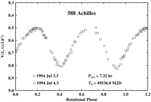
Figure 1. Composite light curve for 588 Achilles during the 1994 apparition.
Download figure:
Standard image High-resolution image659. Nestor
Four nights of observations in 1995 enabled us to measure a reliable rotation period of 15.98 ± 0.03 hr (see Figure 2). The previous estimate, reported by Binzel & Sauter (1992), and based on two nights in 1998, was inaccurate by almost an hour. Hartmann et al. (1988) reported only a light curve amplitude for the 1986 apparition. Quite surprisingly, our determination appears to be the first accurate period measurement published for this comparatively bright object.
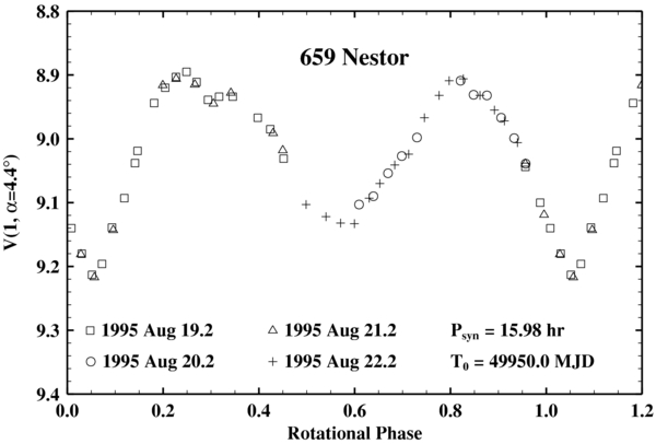
Figure 2. Composite light curve for 659 Nestor during the 1995 apparition.
Download figure:
Standard image High-resolution image884. Priamus
We observed this object during the apparitions of 1993 and 2001. The good sampling and coverage of the light curves resulted in a reliable period determination of about 6.9 hr (see Figures 3 and 4). This object was previously observed photometrically by Hartmann et al. (1988) during four different apparitions between 1983 and 1987. However, the authors reported amplitude estimates but no rotation periods.
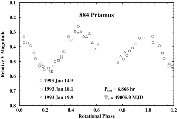
Figure 3. Composite light curve for 884 Priamus during the 1993 apparition.
Download figure:
Standard image High-resolution image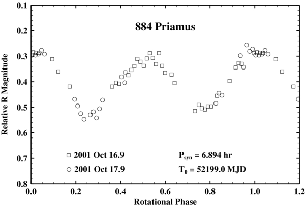
Figure 4. Composite light curve for 884 Priamus during the 2001 apparition.
Download figure:
Standard image High-resolution image911. Agamemnon
Early work by Dunlap & Gehrels (1969), Taylor (1971), and Binzel & Sauter (1992) suggested a rotation period of about 7 hr. More recently, Stephens (2009) found a more precise value of 6.592 ± 0.004 hr, which agrees very well with our determination from 1997 (see Figure 5).

Figure 5. Composite light curve for 911 Agamemnon during the 1997 apparition.
Download figure:
Standard image High-resolution image1143. Odysseus
From our observations spanning four nights in 1994 June we determine a reliable rotation period of 10.111 ± 0.004 hr (see Figure 6), which is in agreement with the determination by Molnar et al. (2008).
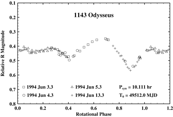
Figure 6. Composite light curve for 1143 Odysseus during the 1994 apparition.
Download figure:
Standard image High-resolution image1172. Aneas
Three nights of observations enabled us to determine an unambiguous rotation period of about 8.7 hr (see Figure 7). For this object only a previous amplitude estimation from the 1986 apparition was published (Hartmann et al. 1988).
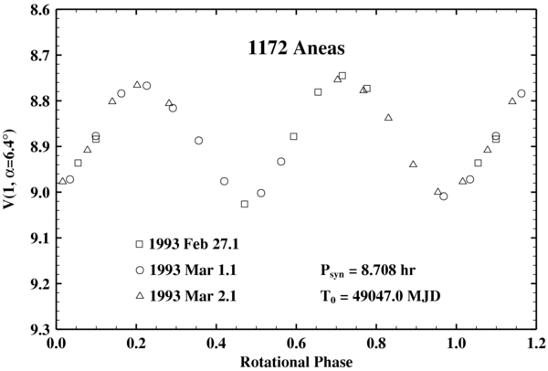
Figure 7. Composite light curve for 1172 Aneas during the 1993 apparition.
Download figure:
Standard image High-resolution image1437. Diomedes
We observed this object for a total of about 22 hr during three nights in 1994 and measured only a slight intensity variation. Sato et al. (2000), in the course of their coordinated occultation campaign in 1997, derived a rotation period of 24.46 hr, an amplitude of 0.70 mag, and a triaxial shape of 284 × 126 × 65 km. We used their period, later confirmed by Stephens (2009), to produce a composite of our data, as shown in Figure 8. Although our data cover as much as 40% of the rotation period, the maximum intensity variation displayed by the observations was only about 0.02 mag. From the shape of the light curve we subjectively estimate that the maximum amplitude during the 1994 apparition had not exceeded 0.1 mag.

Figure 8. Composite light curve for 1437 Diomedes during the 1994 apparition.
Download figure:
Standard image High-resolution image1749. Telamon
Four nights of observations in 1995 August resulted in a reliable rotation period of about 11.12 hr (see Figure 9). No previous period determinations are reported in the literature.
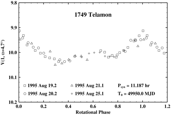
Figure 9. Composite light curve for 1749 Telamon during the 1995 apparition.
Download figure:
Standard image High-resolution image1867. Deiphobus
Earlier observations by French (1987) suggested a rotation period longer than 24 hr. From seven nights in 1994 February we were able to pin the period of this slow rotator down to 58.66 ± 0.18 hr (see Figure 10). Although the period is firmly constrained, the determination of the light curve amplitude is more uncertain, as the shape of one maximum relies on the observations taken on February 9, which are not overlapping with any other.
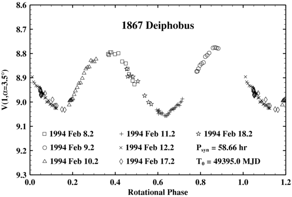
Figure 10. Composite light curve for 1867 Deiphobus during the 1994 apparition.
Download figure:
Standard image High-resolution image1868. Thersites
Three nights in 1994 resulted in a reliable period of 10.4 hr, which is the first value published for this object (see Figure 11).

Figure 11. Composite light curve for 1868 Thersites during the 1994 apparition.
Download figure:
Standard image High-resolution image1873. Agenor
We observed this object during five nights in 1994 February (see Figure 12). The good accuracy and sampling of the measurements enabled us to determine an accurate rotation period notwithstanding the small amplitude and the comparatively long period.
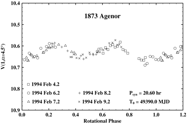
Figure 12. Composite light curve for 1873 Agenor during the 1994 apparition.
Download figure:
Standard image High-resolution image2207. Antenor
Observations during the 1989 and 1996 apparitions show very irregular light curves, characterized by four maxima and four minima in 1989 (see Figure 13), and three maxima and three minima in 1996 (see Figure 14). In Gonano et al. (1991) we listed a preliminary determination of Antenor's rotation period and light curve amplitude based the 1989 observations, which are shown here for the first time. An earlier estimate of the light curve amplitude was published by Hartmann et al. (1988) from the data taken in 1983.
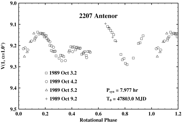
Figure 13. Composite light curve for 2207 Antenor during the 1989 apparition.
Download figure:
Standard image High-resolution image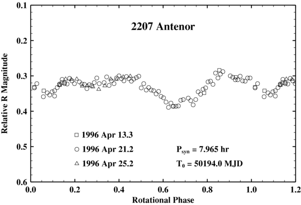
Figure 14. Composite light curve for 2207 Antenor during the 1996 apparition.
Download figure:
Standard image High-resolution image2223. Sarpedon
Observations from the 1994 and 1996 apparitions allowed us to derive a reliable rotation period of about 22.7 hr (see Figures 15 and 16). The near-commensurability with the duration of the Earth day required careful planning of the observations in order to achieve a complete coverage of the light curve. A lower bound for the amplitude, given by Hartmann et al. (1988) based on their unpublished observations of 1984, was the only previous literature information available for this object.

Figure 15. Composite light curve for 2223 Sarpedon during the 1994 apparition.
Download figure:
Standard image High-resolution image
Figure 16. Composite light curve for 2223 Sarpedon during the 1996 apparition.
Download figure:
Standard image High-resolution image2241. Alcathous
Observations from the 1991 apparition reveal a unique rotation period of about 7.7 hr (see Figure 17). An earlier estimation of 9.41 hr published by De Sanctis et al. (1994), based on six nights in 1992 December and 1993 January, corresponds to an alias of the correct period. Hartmann et al. (1988) reported an amplitude estimation for the 1994 apparition.
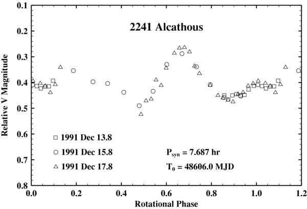
Figure 17. Composite light curve for 2241 Alcathous during the 1991 apparition.
Download figure:
Standard image High-resolution image2260. Neoptolemus
From the apparitions of 1995 and 2002 we determined a unique rotation period of 8.18 hr (see Figures 18 and 19). Binzel & Sauter (1992) had guessed a period longer than 12 hr from their 1988 observations, while Angeli et al. (1999) suggested a period of 8.5 ± 0.1 hr, which, though outside their formal error, is closer to the correct period.
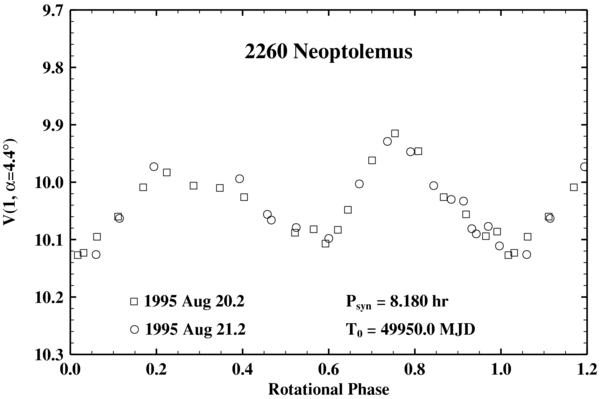
Figure 18. Composite light curve for 2260 Neoptolemus during the 1995 apparition.
Download figure:
Standard image High-resolution image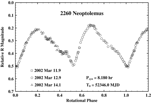
Figure 19. Composite light curve for 2260 Neoptolemus during the 2002 apparition.
Download figure:
Standard image High-resolution image2357. Phereclos
Four nights of observations in 1994 revealed an irregular light curve with a low amplitude (see Figure 20), which made it difficult to estimate the number of cycles elapsed between subsequent nights, and resulted in multiple possible solutions. We observed this object again for seven nights in 2010, which enabled us to identify unambiguously a synodic period of about 14.4 hr (see Figure 21). Hartmann et al. (1988) report an amplitude of 0.14? [sic] for the 1987 apparition, possibly meaning that their determination is either noisy, or derived from an incomplete light curve coverage.
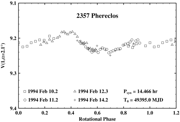
Figure 20. Composite light curve for 2357 Phereclos during the 1994 apparition.
Download figure:
Standard image High-resolution image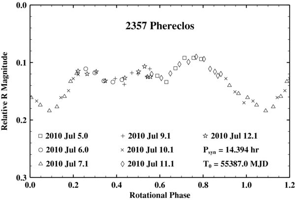
Figure 21. Composite light curve for 2357 Phereclos during the 2010 apparition.
Download figure:
Standard image High-resolution image2363. Cebriones
Five nights of observations in 1994 resulted in a reliable rotation period of 20.05 hr for this object (see Figure 22). Galad & Kornos (2008) report a period of 20.081 hr from their measurements acquired during the 2008 apparition, which is compatible with our determination.
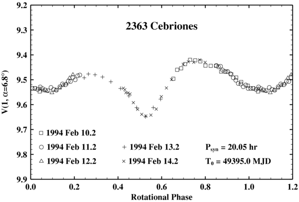
Figure 22. Composite light curve for 2363 Cebriones during the 1994 apparition.
Download figure:
Standard image High-resolution image2456. Palamedes
Our observations during four nights in 1995 June yield a synodic rotation period of 7.258 ± 0.004 hr, with an amplitude of only 0.05 mag (see Figure 23). Stephens (2010) published two nights of observations taken during the 2009 apparition, from which he determined a period of 7.24 ± 0.01 hr, which is in good agreement with our determination.
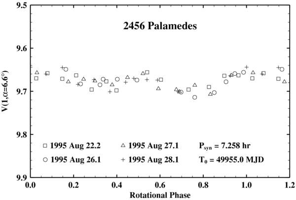
Figure 23. Composite light curve for 2456 Palamedes during the 1995 apparition.
Download figure:
Standard image High-resolution image2674. Pandarus
French (1987) published a period of 8.4803 ± 0.0019 hr and a large light curve amplitude of 0.58 mag from three nights in 1986. Our observations spanning 8 hr with 105 data points from one night in 2001 October revealed virtually no light curve variation (see Figure 24), which implies a near polar view at the time of the observations. We used the French (1987) rotation period to plot our data versus rotational phase.
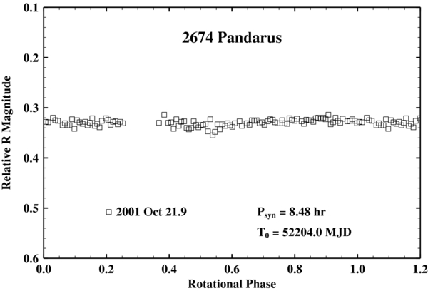
Figure 24. Composite light curve for 2674 Pandarus during the 2001 apparition.
Download figure:
Standard image High-resolution image2759. Idomeneus
Our first data of Idomeneus date back to the apparitions of 1991 and 1992, when we followed this object for a total of seven nights. The individual-night observations revealed a comparatively slow rotation. For this reason, the observations provided only an incomplete coverage of the rotation period and limited overlap among different nights. At that time, we searched for the rotation period that best fitted both sets of observations under the assumption of a double sine-wave light curve, which resulted in a tentative value of about 32 hr. On 2010 December we had again the opportunity to observe Idomeneus, which allowed us to unambiguously confirm and refine its period to Psyn = 32.38 hr (see Figure 27). The observations of 1991 and 1992 are also folded with this period (see Figures 25 and 26).

Figure 25. Composite light curve for 2759 Idomeneus during the 1991 apparition.
Download figure:
Standard image High-resolution image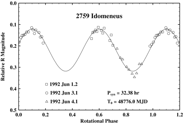
Figure 26. Composite light curve for 2759 Idomeneus during the 1992 apparition.
Download figure:
Standard image High-resolution image
Figure 27. Composite light curve for 2759 Idomeneus during the 2010 apparition.
Download figure:
Standard image High-resolution image2895. Memnon
Our observations during three nights in 1990 November yield a reliable rotation period of 7.502 ± 0.010 hr (see Figure 28). Binzel & Sauter (1992) observed this object for 5 hr during a single night in 1990, from which they guessed a correct period of 7.5 hr.
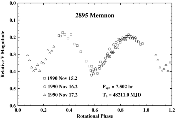
Figure 28. Composite light curve for 2895 Memnon during the 1990 apparition.
Download figure:
Standard image High-resolution image2920. Automedon
Four nights of observations in 1994 allowed us to determine an unambiguous rotation period of 10.220 ± 0.004 hr (see Figure 29), which is in excellent agreement with the determination by Molnar et al. (2008).
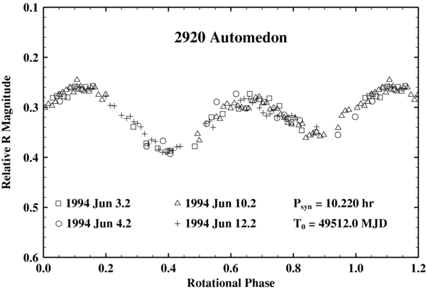
Figure 29. Composite light curve for 2920 Automedon during the 1994 apparition.
Download figure:
Standard image High-resolution image3063. Makhaon
We observed 3063 Makhaon in two apparitions, during which the asteroid displayed a small light curve amplitude. As it often happens in these cases, the light curve was very irregular, with multiple maxima and minima. We found a unique solution that best fits both apparitions with a rotation period of about 8.6 hr (see Figures 30 and 31). The resulting rotation coverage is complete and the reproducibility of the measurements on subsequent nights is good.

Figure 30. Composite light curve for 3063 Makhaon during the 1994 apparition.
Download figure:
Standard image High-resolution image
Figure 31. Composite light curve for 3063 Makhaon during the 2009 apparition.
Download figure:
Standard image High-resolution imageThis object was also observed by Binzel & Sauter (1992) in 1988, who collected light curves during two consecutive nights of observations. Based on these data, the authors suggested a period of 17.3 hr, under the assumption of a two-maximum two-minimum light curve. We have composited the data by Binzel & Sauter with our period and we obtained an excellent fit. At the time of their observations, 3063 was characterized by a prominent maximum–minimum feature, and displayed only a hint of a secondary maximum and minimum, which led the authors to derive a period double as long as the real one.
3240. Laocoon
We observed this object during two nights in 1996 April from which a reliable period of 11.312 ± 0.014 hr could be determined (see Figure 32). For this object only an amplitude estimate was previously available (Hartmann et al. 1988).

Figure 32. Composite light curve for 3240 Laocoon during the 1996 apparition.
Download figure:
Standard image High-resolution image3317. Paris
We observed Paris during three nights in 1990 November when the object displayed a low amplitude and a very irregular shape (see Figure 33). The anomalous number of maxima and minima made it difficult at that time to estimate the fundamental periodicity. For this reason, we observed the object again for five nights in 1998, from which we could determine an unambiguous synodic period of 7.082 ± 0.003 hr (see Figure 34). Behrend (2010) reports on his Web page independent observations by René Roy and by Federico Manzini, who derive a rotation period compatible with our determination.
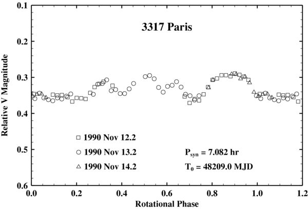
Figure 33. Composite light curve for 3317 Paris during the 1990 apparition.
Download figure:
Standard image High-resolution image
Figure 34. Composite light curve for 3317 Paris during the 1998 apparition.
Download figure:
Standard image High-resolution image3451. Mentor
We observed this object during the apparitions of 1993 and 1998, from which we derived a period of 7.7 hr (see Figures 35 and 36). A series of earlier period determinations, all compatible with our value, have been published (Sauppe et al. 2007; Duffard et al. 2008; Melita et al. 2010). In addition, light curves by several authors have been published online by Behrend (2010). An amplitude estimate from observations in 1987 can be found in Hartmann et al. (1988).

Figure 35. Composite light curve for 3451 Mentor during the 1993 apparition.
Download figure:
Standard image High-resolution image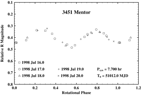
Figure 36. Composite light curve for 3451 Mentor during the 1998 apparition.
Download figure:
Standard image High-resolution image3548. Eurybates
We observed this object during the 1992 apparition for four nights and derived an unambiguous rotation period of 8.711 hr (see Figure 37). Stephens (2010) reports his own observations of 3548 Eurybates during two nights in the 2009 opposition that enabled him to independently determine a rotation period of 8.73 hr. The two determinations are in excellent agreement, within the respective uncertainties.

Figure 37. Composite light curve for 3548 Eurybates during the 1992 apparition.
Download figure:
Standard image High-resolution imageAt the time of Stephens' observations, the asteroid was located at an ecliptic longitude almost exactly 180° apart from that during our observations. This coincidence resulted in very similar viewing conditions, and consequently, similar light curve shapes and amplitudes.
3564. Talthybius
Six nights of observations in 1994 June resulted in a composite with a complete coverage for this comparatively slow rotator (see Figure 38). The unambiguous period of 40.59 ± 0.13 hr is in agreement with the recent determination by Stephens (2010).
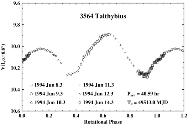
Figure 38. Composite light curve for 3564 Talthybius during the 1994 apparition.
Download figure:
Standard image High-resolution image3708. 1974 FV1
Three nights of observations in 1993 resulted in an unambiguous period of 6.55 hr (see Figure 39). No previous period determinations have been published for this object.
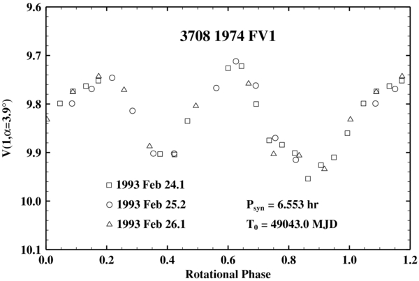
Figure 39. Composite light curve for 3708 1974 FV1 during the 1993 apparition.
Download figure:
Standard image High-resolution image3793. Leonteus
In 1994, this object displayed a regular two-maximum two-minimum light curve with a period of 5.62 hr and an amplitude of 0.24 mag (see Figure 40). In 1997, the object had a much smaller amplitude and a single maximum–minimum light curve (see Figure 41). Stephens (2010) reports his observations of 2009, during which the viewing geometry was very close to that of 1997. For this reason the one-maximum one-minimum appearance of the light curve led Stephens to estimate a wrong rotation period of 11.22 hr.
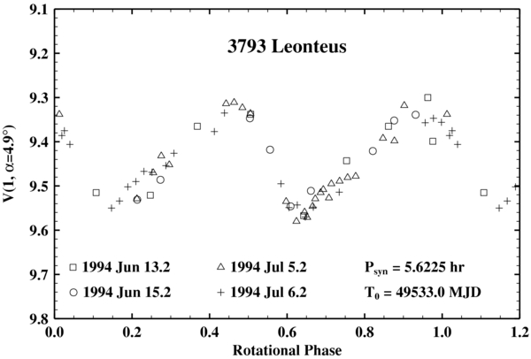
Figure 40. Composite light curve for 3793 Leonteus during the 1994 apparition.
Download figure:
Standard image High-resolution image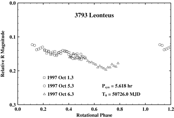
Figure 41. Composite light curve for 3793 Leonteus during the 1997 apparition.
Download figure:
Standard image High-resolution image3794. Sthenelos
Four nights of observations in 1995 August allowed us to determine the rotation period of this object (see Figure 42). Quick-look data reduction at the telescope allowed us to schedule the observations to cover the whole period, despite the near 2:1 commensurability with the length of the Earth day.

Figure 42. Composite light curve for 3794 Sthenelos during the 1995 apparition.
Download figure:
Standard image High-resolution image4007. Euryalos
We observed Euryalos in 1995 for four nights (see Figure 43). Despite the low amplitude displayed during that apparition, we could determine a reliable rotation period, which constitutes the first determination published for this object.
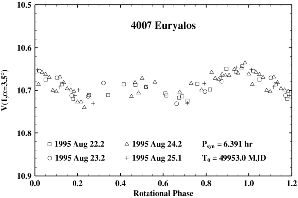
Figure 43. Composite light curve for 4007 Euryalos during the 1995 apparition.
Download figure:
Standard image High-resolution image4035. 1986 WD
We observed this object for the first time during two nights in 1991 May (see Figure 44). From these observations alone, however, an unambiguous rotation period could not be derived, due to the difficulty in the estimation of the elapsed cycles between the observations. In 2009, we had a second opportunity to observe 1986 WD, which finally resulted in a solid determination of 13.467 hr (see Figure 45). The object displays a peculiar light curve, with a bilobated secondary maximum. By chance, during the observations of 1991 and 2009 the object was visible from Earth from almost exactly opposite directions. For this reason, the shape of the light curve during the two apparitions is very similar. No previous period determinations are available in the literature for this object.
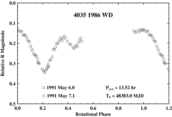
Figure 44. Composite light curve for 4035 1986 WD during the 1991 apparition.
Download figure:
Standard image High-resolution image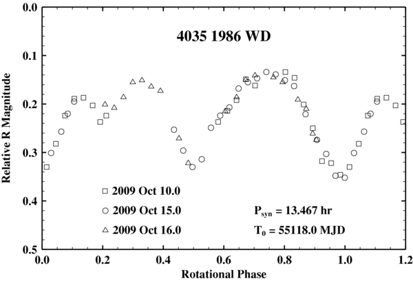
Figure 45. Composite light curve for 4035 1986 WD during the 2009 apparition.
Download figure:
Standard image High-resolution image4057. Demophon
We derive a period of 29.31 ± 0.07 hr from six nights of observations in 1994 (see Figure 46). The only previous published determination for this object is an amplitude estimation for the 1986 apparition by Hartmann et al. (1988).

Figure 46. Composite light curve for 4057 Demophon during the 1994 apparition.
Download figure:
Standard image High-resolution image4063. Euforbo
From two consecutive nights in 1992, showing two maxima and one minimum, and one maximum and two minima, respectively, we could determine a reliable period for Euforbo, which constitutes its first period determination published (see Figure 47).

Figure 47. Composite light curve for 4063 Euforbo during the 1992 apparition.
Download figure:
Standard image High-resolution image4086. Podalirius
We observed Podalirius on three consecutive nights in 1991 May, from which we derived a best-fit period of 10.43 hr (see Figure 48). Stephens (2009) reports his observations of this object during two consecutive nights in 2008 October, and on a third night one week later. From these data he derives a period of 14.51 hr, which corresponds approximately to a 3.5:5 alias of our period. We plotted R. D. Stephens' original data (2009, private communication) with our own period of 10.43 hr, and actually obtained a better solution than that published in the original reference. With our period, Stephens' composite displays only one maximum and one minimum, and perhaps for this reason, the author had rejected the correct solution.

Figure 48. Composite light curve for 4086 Podalirius during the 1991 apparition.
Download figure:
Standard image High-resolution image4348. Poulydamas
Three nights of observations in 1990 resulted in an unambiguous rotation period of about 9.9 hr (see Figure 49). No other determinations have been previously published for this object.
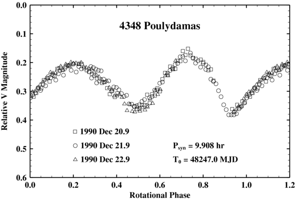
Figure 49. Composite light curve for 4348 Poulydamas during the 1990 apparition.
Download figure:
Standard image High-resolution image4489. 1988 AK
Four consecutive nights of observations in 1995 August revealed a light curve with an extremely low amplitude and an irregular shape. The Fourier analysis produced two possible periods around 16.2 hr and 12.6 hr, with the former having a slightly higher significance. Because of the very low amplitude, however, combined with the uncertainty about the number of maxima and minima, a certain period determination was not possible. For this reason, we re-observed this object for 10 nights during the 2010 apparition, when, due to a different viewing geometry, the object happened to display a larger amplitude. These latter observations (see Figure 51) allowed us to determine an unambiguous period of 12.582 hr, which represents the first published value for this object. This period was also used to produce the composite for the 1995 observations (see Figure 50), during which the object must have shown us a near polar view.

Figure 50. Composite light curve for 4489 1988 AK during the 1995 apparition.
Download figure:
Standard image High-resolution image
Figure 51. Composite light curve for 4489 1988 AK during the 2010 apparition.
Download figure:
Standard image High-resolution image4543. Phoinix
This object was observed from two stations for a total of 12 nights over a time span of about seven weeks during the winter of 2009 (see Figure 52). Even though due to the long rotation period and to bad weather we covered only about 74% of the light curve, the derived period solution is unique. This is partly due to the fact that, whenever possible, we made use of the same set of comparison field stars on consecutive nights, which, by reducing the number of parameters fitted, makes the solution more stable, especially for long rotation periods.
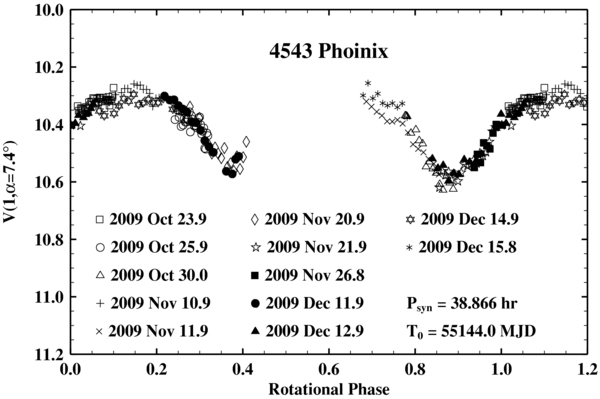
Figure 52. Composite light curve for 4543 Phoinix during the 2009 apparition.
Download figure:
Standard image High-resolution image4709. Ennomos
Five nights of observations in 1990 enabled us to determine an unambiguous rotational period for this object (see Figure 53). Because the period is close to 12 hr, near real-time data reduction was key to planning the following nights' observations, which helped us achieve a complete rotational coverage.

Figure 53. Composite light curve for 4709 Ennomos during the 1990 apparition.
Download figure:
Standard image High-resolution image4715. 1989 TS1
We observed this object during four nights in 1991 and unambiguously determined its rotation period (see Figure 54), which represents the first value published for this object.

Figure 54. Composite light curve for 4715 1989 TS1 during the 1991 apparition.
Download figure:
Standard image High-resolution image4722. Agelaos
From observations on two consecutive nights in 2002 December we determined a rotation period of about 18.6 hr. Although the composite covers only about 75% of the complete period (see Figure 55), and there is no overlap between the two nights, the solution is unique. During the two nights, the same set of in-field comparison stars was observed, so that no arbitrary magnitude shift was applied to compile the composite. No previous determinations have been published for this object.
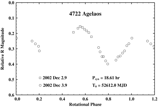
Figure 55. Composite light curve for 4722 Agelaos during the 2002 apparition.
Download figure:
Standard image High-resolution image4754. Panthoos
Seven consecutive nights of observations in 1994 February enabled us to determine and completely cover the rotation period of this comparatively slow rotator (see Figure 56). This is the first determination published for this object.
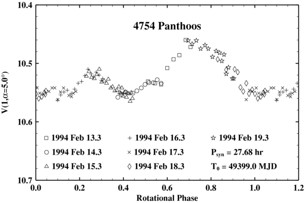
Figure 56. Composite light curve for 4754 Panthoos during the 1994 apparition.
Download figure:
Standard image High-resolution image4791. Iphidamas
From two runs, in 1991 and 1993, we could determine an unambiguous rotation period of about 9.73 hr. During the 1991 apparition, the object displayed only one maximum and one minimum in its light curve (see Figure 57), while in 1993 it showed two pairs of extrema (see Figure 58).
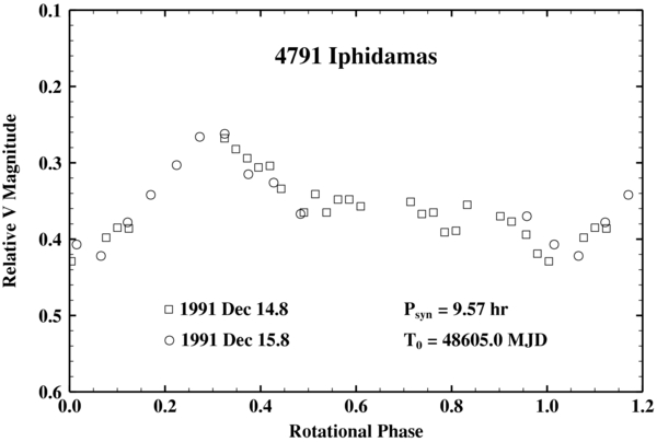
Figure 57. Composite light curve for 4791 Iphidamas during the 1991 apparition.
Download figure:
Standard image High-resolution image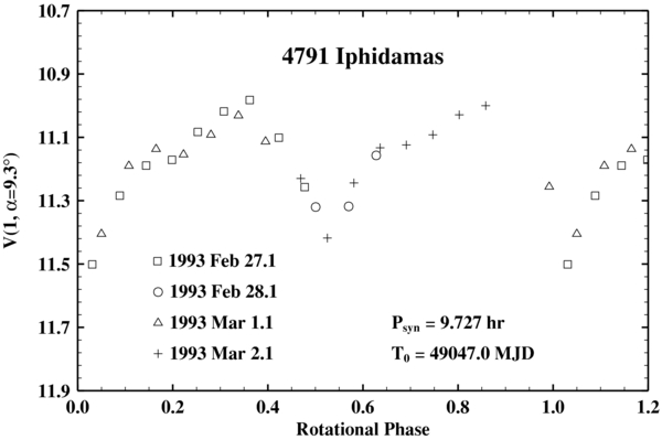
Figure 58. Composite light curve for 4791 Iphidamas during the 1993 apparition.
Download figure:
Standard image High-resolution image4792. Lykaon
A total of six nights of observations allowed us to determine a rotation period of about 40 hr for this object, under the assumption of two maxima and two minima per rotation cycle (see Figure 59). The observations taken during the night of 1996 April 19, which cover the secondary maximum of the light curve, do not overlap with observations from any other nights. For this reason, the amplitude of the secondary maximum is not well constrained. No previous photometric measurements are reported in the literature for this object.
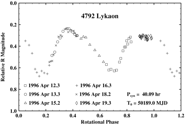
Figure 59. Composite light curve for 4792 Lykaon during the 1996 apparition.
Download figure:
Standard image High-resolution image4805. Asteropaios
Four nights of observations in 1994 February provided full coverage of the rotational cycle of this object, enabling us to determine an unambiguous period of about 12.4 hr (see Figure 60). This represents the first determination published for Asteropaios.
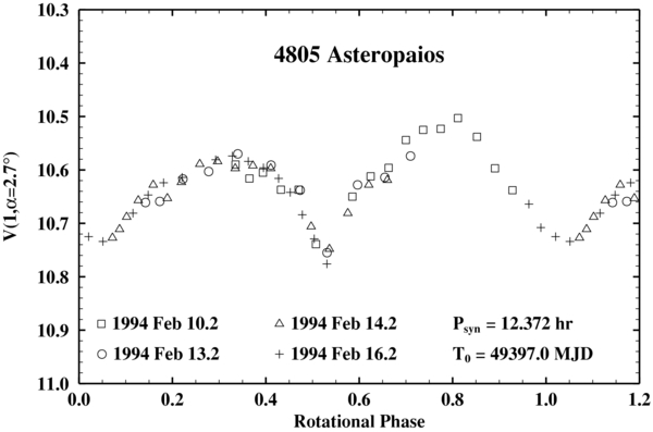
Figure 60. Composite light curve for 4805 Asteropaios during the 1994 apparition.
Download figure:
Standard image High-resolution image4827. Dares
Five nights of observations resulted in multiple coverage of the rotation period of nearly 19 hr (see Figure 61), which represents the first determination published for Dares.
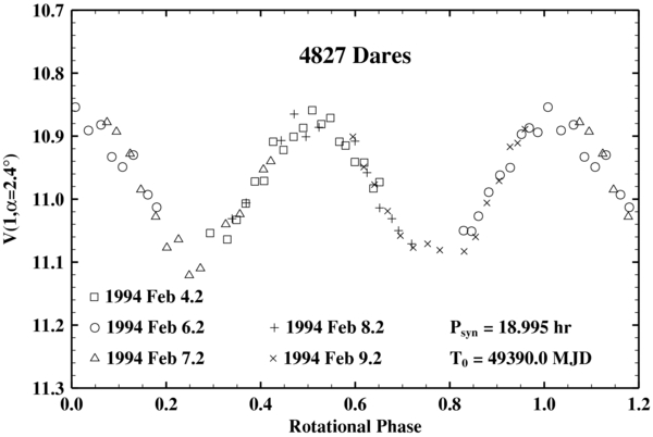
Figure 61. Composite light curve for 4827 Dares during the 1994 apparition.
Download figure:
Standard image High-resolution image4828. Misenus
We observed Misenus for three nights in 1995. From a well-sampled light curve we could determine an unambiguous period of about 12.9 hr (see Figure 62), which represents the first estimate published for this object.

Figure 62. Composite light curve for 4828 Misenus during the 1995 apparition.
Download figure:
Standard image High-resolution image4832. Palinurus
We observed this object during eight consecutive nights of observations in 2010 (see Figure 63). However, due to the comparatively low amplitude of the light curve, and to the rather noisy data set due to the object being located in a crowded field, it was difficult to estimate the number of cycles elapsed per night. Therefore, the resulting best-fit period of about 5.3 hr should be regarded as tentative.
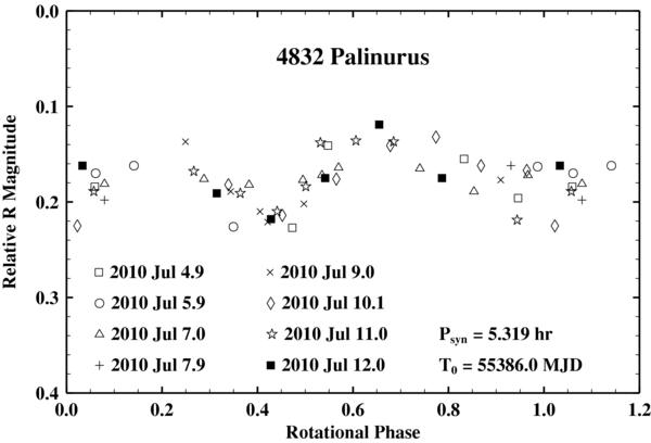
Figure 63. Composite light curve for 4832 Palinurus during the 2010 apparition.
Download figure:
Standard image High-resolution image4833. Meges
Four nights in 1995 August resulted in a reliable period of 14.25 hr (see Figure 64). No other photometric measurements have been published for this object to date.

Figure 64. Composite light curve for 4833 Meges during the 1995 apparition.
Download figure:
Standard image High-resolution image4834. Thoas
During four nights of observations in 1996 September the object displayed an asymmetric light curve with a subdued secondary minimum (see Figure 65). An unambiguous period of about 18.2 hr represents the first determination published for this object.

Figure 65. Composite light curve for 4834 Thoas during the 1996 apparition.
Download figure:
Standard image High-resolution image4836. Medon
We observed this object for the first time during its 1991 apparition. The asteroid displayed an irregular light curve with the presence of additional maxima and minima (see Figure 66), which made it difficult to estimate the fundamental periodicity. Two solutions were equally likely. In order to resolve this ambiguity we re-observed this object during two more apparitions, that of 1992 (see Figure 67) and of 2009–2010 (see Figures 68 and 69), which confirmed the 9.84 hr period. No previous observations of this object are reported in the literature.

Figure 66. Composite light curve for 4836 Medon during the 1991 apparition.
Download figure:
Standard image High-resolution image
Figure 67. Composite light curve for 4836 Medon during the 1992 apparition.
Download figure:
Standard image High-resolution image
Figure 68. Composite light curve for 4836 Medon during the 2009 apparition.
Download figure:
Standard image High-resolution image
Figure 69. Composite light curve for 4836 Medon during the 2010 apparition.
Download figure:
Standard image High-resolution image4946. Askalaphus
Askalaphus was observed during its 1992 apparition. After the first few nights it became apparent that the rotation period was close to 24 hr (see Figure 70). As a consequence, the following observations were carefully planned to allow for a complete coverage of the light curve. The resulting period is unambiguous and represents the first determination for this object published in the literature.

Figure 70. Composite light curve for 4946 Askalaphus during the 1992 apparition.
Download figure:
Standard image High-resolution image5023. Agapenor
We observed this object for five nights in 2009 September. The best-fit period is 5.4 hr, and the resulting light curve is characterized by the presence of very subtle secondary maxima, in addition to the primary ones (see Figure 71). A solution with exactly half the period, although formally less probable, could also be possible. This solution would result in a light curve with a primary maximum and a subdued secondary maximum. In order to resolve this ambiguity, observations from different geometries would be desirable, in order to monitor the evolution of the shape of the light curve as a function of the viewing direction. Should the shorter period be confirmed, this would represent the fastest rotator among the Trojans observed so far.
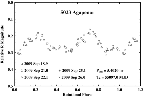
Figure 71. Composite light curve for 5023 Agapenor during the 2009 apparition.
Download figure:
Standard image High-resolution image5025. 1986 TS6
This object was observed for eight nights during its 2009 apparition. During each night, mostly constant slopes were observed, with significant brightness variations from night to night, which was suggestive of a long period (see Figure 72). In order to estimate the rotation period, we fitted the data to a sine wave. We divided the observations into three groups of adjacent nights, where the observations within each group were referenced to the same set of in-field comparison stars. The fit, which involved solving for three parameters (two magnitude offsets and the period), results in a rotation period exceeding 10 days. Although this period requires confirmation, we believe that this object is among the slowest Trojans observed so far. In the case where 5025 has no companion, its rotation state might be excited, as the damping times for an object of this size are of the order of a few billion years (Harris 1994).

Figure 72. Composite light curve for 5025 1986 TS6 during the 2009 apparition.
Download figure:
Standard image High-resolution image5027. Androgeos
Androgeos was observed for three nights during its 1992 apparition, which resulted in an unambiguous rotation period of 11.355 hr (see Figure 73). No other photometric measurements are reported in the literature for this object.

Figure 73. Composite light curve for 5027 Androgeos during the 1992 apparition.
Download figure:
Standard image High-resolution image5028. Halaesus
A reliable rotation period just under 25 hr was measured for this object in six nights of observations in 1996 (see Figure 74). This represents the only period determination available for this object in the literature.
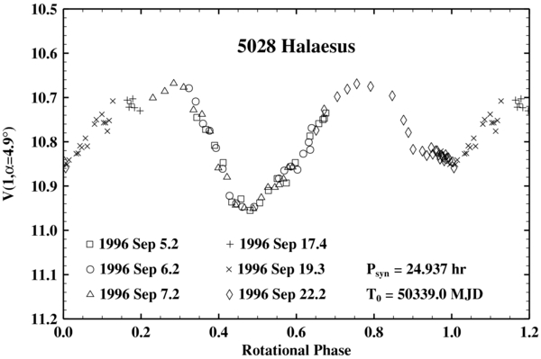
Figure 74. Composite light curve for 5028 Halaesus during the 1996 apparition.
Download figure:
Standard image High-resolution image5119. 1988 RA1
A literature search revealed no previous period determinations for this objects, for which we measured an unambiguous period of 12.807 hr during three nights of observations in 1992 (see Figure 75).

Figure 75. Composite light curve for 5119 1988 RA1 during the 1994 apparition.
Download figure:
Standard image High-resolution image5120. Bitias
We observed Bitias during four consecutive nights in 1993 and derived a period of 11.58 hr. Since the period is close to 12 hr, however, we could only cover about 70% of the light curve (see Figure 76).
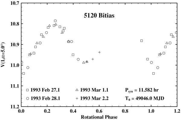
Figure 76. Composite light curve for 5120 Bitias during the 1993 apparition.
Download figure:
Standard image High-resolution image5130. Ilioneus
Five nights of observations in 1994 completely sampled the object's light curve multiple times, providing an unambiguous rotation period of about 14.8 hr (see Figure 77). No previous results have been published for this object.
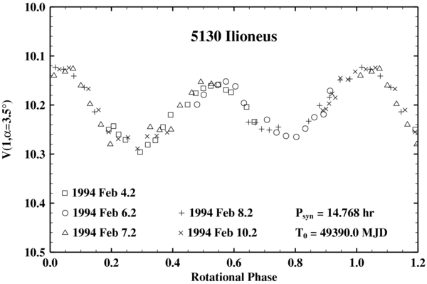
Figure 77. Composite light curve for 5130 Ilioneus during the 1994 apparition.
Download figure:
Standard image High-resolution image5144. Achates
From three nights in April 1996 we derived a period of 5.949 ± 0.014 hr (see Figure 78), in good agreement with the recent determination by Molnar et al. (2008).
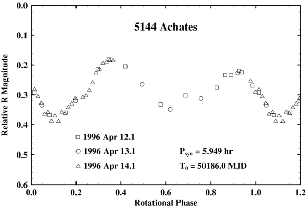
Figure 78. Composite light curve for 5144 Achates during the 1996 apparition.
Download figure:
Standard image High-resolution image5254. Ulysses
Five nights of observations in 1996 completely covered its light curve, despite the relatively slow rotation (see Figure 79). We determine an unambiguous period of 28.72 hr, which represents the first period determination published for this object.

Figure 79. Composite light curve for 5254 Ulysses during the 1996 apparition.
Download figure:
Standard image High-resolution image5259. Epeigeus
Five consecutive nights of observations in 1995 August resulted in a best-fit period of 18.51 hr for this object, which displays an irregular light curve with a comparatively low amplitude (see Figure 80).
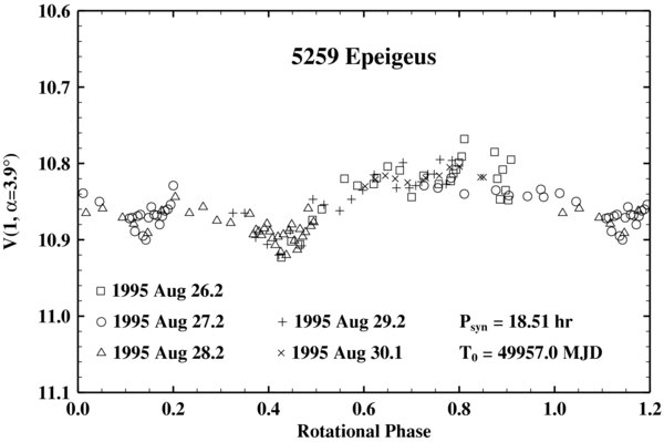
Figure 80. Composite light curve for 5259 Epeigeus during the 1995 apparition.
Download figure:
Standard image High-resolution image5264. Telephus
Telephus was observed for four nights in 1994, yielding a reliable rotation period of 9.518 hr (see Figure 81), which represents the first period determination published for this object.

Figure 81. Composite light curve for 5264 Telephus during the 1994 apparition.
Download figure:
Standard image High-resolution image5283. Pyrrhus
We first observed this object during one night in 1996, when it showed very little light curve variation (see Figure 82). For this reason, we observed it again at our next opportunity, in 2002 March, when we could determine a reliable period of 7.323 hr (see Figure 83). We also used this period, which represents the first published determination for Pyrrhus, for plotting our observations of 1996, which turned out to cover the whole rotation in one night.

Figure 82. Composite light curve for 5283 Pyrrhus during the 1996 apparition.
Download figure:
Standard image High-resolution image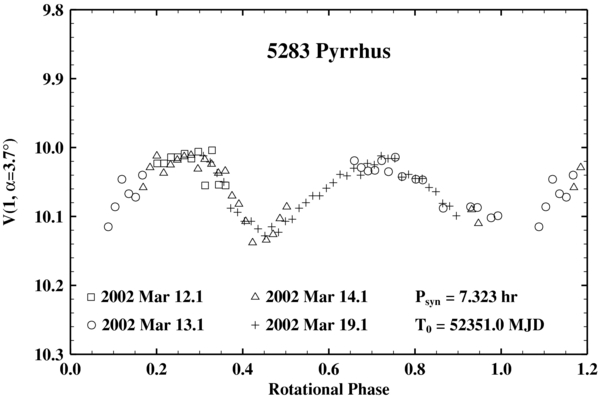
Figure 83. Composite light curve for 5283 Pyrrhus during the 2002 apparition.
Download figure:
Standard image High-resolution image5476. 1989 TO11
Four nights of observations in 1994 revealed a regular light curve with moderate amplitude and an unambiguous period of 5.78 hr (see Figure 84), which represents the first period determination published for this object.

Figure 84. Composite light curve for 5476 1989 TO11 during the 1994 apparition.
Download figure:
Standard image High-resolution image5511. Cloanthus
Observations during the 2010 apparition revealed only minor intensity variations during each individual night. The object, however, displayed large night-to-night variations, which hinted at a long rotation period. Thanks to the large detector field of view, it was possible to observe the same sets of in-field comparison stars during consecutive nights, which enabled us to accurately refer all of the observations to the same magnitude scale. Fitting a sine wave to the data results in a rotation period of about 14 days (see Figure 85). This object represents an interesting target for follow-up observations, being a potential complex rotator.

Figure 85. Composite light curve for 5511 Cloanthus during the 2010 apparition.
Download figure:
Standard image High-resolution image5638. Deikoon
From six nights of observations in 1994 we derived a reliable rotation period of 9.137 ± 0.003 hr (see Figure 86). The object displays an irregular light curve with an amplitude of only 0.07 mag. Our determination rules out the tentative period published by Molnar et al. (2008).

Figure 86. Composite light curve for 5638 Deikoon during the 1994 apparition.
Download figure:
Standard image High-resolution image5648. 1990 VU1
We observed this object for eight nights in 2009, which allowed us to determine an unambiguous period of 37.56 hr (see Figure 87). Despite the long rotation period, we covered about 80% of the rotation. Groups of two consecutive nights referred to the same in-field comparison stars. As a consequence, all observation groups share some overlap, and no arbitrary magnitude shift was used. Behrend (2010) reports on his Web page observations by Federico Manzini during three nights in the 2005 apparition; Manzini derived a rotation period of about 16 hr, which is incompatible with our determination.
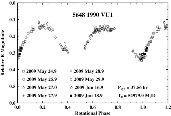
Figure 87. Composite light curve for 5648 1990 VU1 during the 2009 apparition.
Download figure:
Standard image High-resolution image6002. 1988 RO
Three nights of observations in 1993 February provided full coverage of the rotation of this object (see Figure 88). The period of 12.918 hr represents its first determination published in the literature.
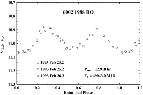
Figure 88. Composite light curve for 6002 1988 RO during the 1993 apparition.
Download figure:
Standard image High-resolution image6090. 1989 DJ
Our first observations of this object, which were performed during five consecutive nights in 1994, revealed a very tortuous light curve with multiple features having a small amplitude (see Figure 89). The best-fit period of about 18.6 hr produced excellent residuals, but was considered ambiguous because of the uncertain number of extrema occurring per cycle. Further observations, acquired during our next opportunity in 2009, captured a light curve with a higher amplitude, where the multiple features were easily identifiable across different cycles (see Figure 90). These observations allowed us to confirm our first determination of the rotation period.
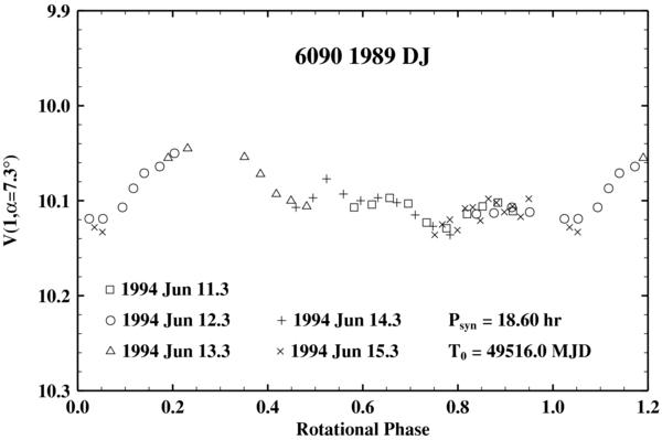
Figure 89. Composite light curve for 6090 1989 DJ during the 1994 apparition.
Download figure:
Standard image High-resolution image
Figure 90. Composite light curve for 6090 1989 DJ during the 2009 apparition.
Download figure:
Standard image High-resolution image7119. Hiera
We observed Hiera for five consecutive nights in 2009. The object displayed only very little variation during each single night. The night-to-night intensity, however, showed a gentle, systematic decreasing trend of about 0.1 mag over five days (see Figure 91), which was measured by referring the solar phase-corrected observations to the same sets of in-field comparison stars. We cannot completely rule out that such a trend of a few percent per day may be due to instrumental effects (as a systematic gradient in the flat fields would cause). However, should the observed light curve variation be confirmed to be solely due to the body's rotation, this would imply a rotation period longer than about 400 hr.

Figure 91. Individual light curves for 7119 Hiera during the July 2009 apparition.
Download figure:
Standard image High-resolution image7641. 1986 TT6
Six nights of observations in 2009 completely covered the comparatively long rotation of this object (see Figure 92). A reliable period of about 27.8 hr represents the first determination published for this object.
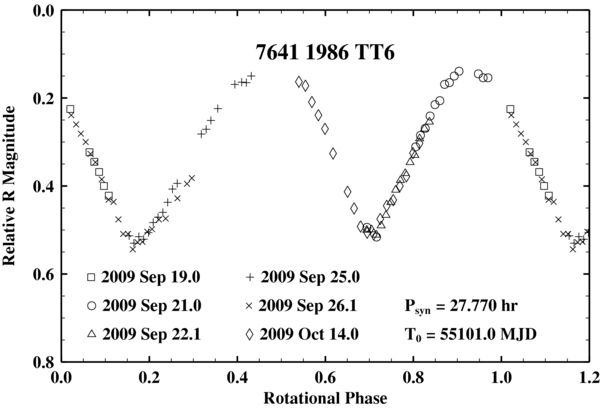
Figure 92. Composite light curve for 7641 1986 TT6 during the 2009 apparition.
Download figure:
Standard image High-resolution image9799. 1996 RJ
We determined a reliable period of about 21.5 hr for this object from six nights of observations in 2009 (see Figure 93). The complete and multiple coverage of its single-peaked light curve makes the determination unambiguous.

Figure 93. Composite light curve for 9799 1996 RJ during the 2009 apparition.
Download figure:
Standard image High-resolution image11395. 1998 XN77
We first observed this asteroid for three consecutive nights in 2009 December. A first period search gave a result of 17.5 hr as the shortest possible period with a two-maximum, two-minimum light curve. Due to the low amplitude and the marginal overlap, however, we considered the period to be tentative. For this reason, this object was assigned a high priority on our target list, and was re-observed during the next opportunity in 2010 November for a total of seven nights (see Figure 95). The latter observations enabled us to determine an unambiguous synodic rotation period of about 13.7 hr. Re-analysis of the 2009 observations (see Figure 94) also showed the correct 13.7 hr solution, which was, however, previously discarded because it resulted in a single maximum–minimum light curve.

Figure 94. Composite light curve for 11395 1998 XN77 during the 2009 apparition.
Download figure:
Standard image High-resolution image
Figure 95. Composite light curve for 11395 1998 XN77 during the 2010 apparition.
Download figure:
Standard image High-resolution image11509. Thersilochos
Six nights of observations in 2010 (see Figure 96) produced a well-sampled composite which resulted in an unambiguous synodic period of about 17.4 hr and which represents the first period determination published for this object.
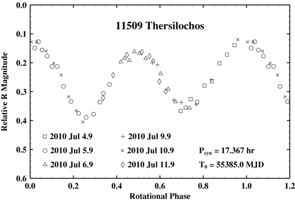
Figure 96. Composite light curve for 11509 Thersilochos during the 2010 apparition.
Download figure:
Standard image High-resolution image12929. 1999 TZ1
From seven nights in 2009 May–June we derived a unique rotation period of 9.2749 ± 0.0016 hr (see Figure 97). Moullet et al. (2008) report previous optical observations for this object. From their sparse data set the authors suggest a period of 5.2 hr or 10.4 hr, under the assumption of a single or double-peaked light curve, respectively. Neither period is, however, compatible with our data.

Figure 97. Composite light curve for 12929 1999 TZ1 during the 2009 apparition.
Download figure:
Standard image High-resolution image16974. 1998 WR21
Seven nights of observations in 2009 October unveiled a slow rotator with a period of about 3.3 days (see Figure 98). When compiling the composite, we linked consecutive nights which shared the same sets of in-field comparison stars. For this reason, although the composite covers about 75% of the whole rotation, all linked groups overlap, making arbitrary magnitude shifts unnecessary. This rotation period, which represents the first determination published for this object, is unambiguous.
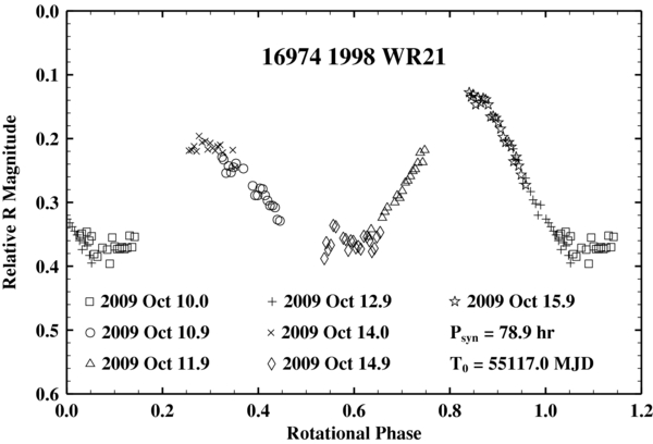
Figure 98. Composite light curve for 16974 1998 WR21 during the 2009 apparition.
Download figure:
Standard image High-resolution image20729. 1999 XS143
This object was observed for five nights on 2009 October. During this apparition the light curve displayed a moderate amplitude and was characterized by a subdued secondary maximum and minimum (see Figure 99). From these observations we derive an unambiguous period of 7.631 hr.
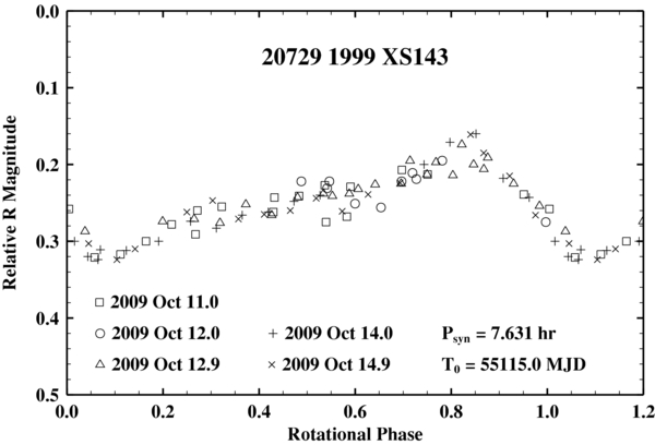
Figure 99. Composite light curve for 20729 1999 XS143 during the 2009 apparition.
Download figure:
Standard image High-resolution imageMelita et al. (2010) report observations of this object performed for two consecutive nights in 2008 when the object showed a much higher amplitude. The authors reported a rotation period of 5.72 hr which is incompatible with our observations, and corresponds exactly to three fourths of the correct period. The probable reason for the disagreement is that the observations by Melita and coauthors, by covering only two time series of about 4.5 hr each, provide only incomplete coverage of the whole rotation. This led the authors to misjudge the number of rotation cycles between the two nights. By using the correct number of elapsed cycles (4), the observations by Melita et al. produce the correct period.
21900. 1999 VQ10
Two consecutive nights totaling about 18 hr of observations result in a rotation period of 13.44 ± 0.08 hr under the assumption of two maxima and two minima per cycle (see Figure 100). No previous observations of this object are reported in the literature.

Figure 100. Composite light curve for 21900 1999 VQ10 during the 2009 apparition.
Download figure:
Standard image High-resolution image
5. SUMMARY
We have carried out a photometric survey of the rotational properties of Jupiter Trojan asteroids. The survey was designed to maximize the reliability of the determinations and to minimize observational bias. The latter was achieved by prioritizing observations of objects for which only inconclusive results were achieved. As a result, out of 80 Trojans observed, we derived new rotational periods for 56 objects, confirmed 13 previously published values, refined one period, and ruled out nine erroneous determinations. Although a thorough analysis of the rotational properties of the Trojans is the subject of a companion paper, we note that during our observations we recorded no extreme light curve amplitudes, with the largest being that of 3240 Lacoon with 0.55 mag. Furthermore, none of our objects showed a rotation faster than about 5.3 hr, a result that might have implications for the density, internal strength, and collisional evolution of these bodies. On the other hand, for about 5% of the objects we measured a period longer than 2 days, with two objects possibly showing a period longer than 14 days. Notwithstanding the considerable effort needed for observing these objects, it is fundamental to continue to follow up these slow rotators in order to understand the causes of their rotation state (Mann et al. 2007; Pravec & Harris 2000).
As a side note, we would like to mention that about 35% of the literature periods that we independently observed proved to be wrong. One possible way to improve this situation would be to re-establish an internet-based repository of light curve data similar to the Standard Asteroid Photometric Catalogue (Torppa 2008) with a user-friendly interface that would enable individual researchers to easily access and share light curve data and cross-check results (Stephens et al. 2010).
The authors are indebted to the many individuals who provided assistance over the years for the observations presented in this paper. In particular, we thank E. Braatz, E. Koldewey, E. Nagel, A. Nathues, G. Pupillo, and S. Hellmich for their help at the telescope. R. D. Stephens is gratefully acknowledged for providing us with his published observations of 4086 Podalirius in digital form.