
ABSTRACT
This article describes a novel calibration method developed for the All Sky Infrared Visible Analyzer (ASIVA). This instrument is principally designed to characterize sky conditions for purposes of improving ground-based astronomical observational performance. Calibration and detection performance of the ASIVA's mid-infrared camera subsystem with particular emphasis on data products that are being developed to quantify photometric quality are described in detail. This analysis allows for the determination of a sky quality metric that can serve as a consistent and reliable metric for telescope scheduling purposes.
Export citation and abstract BibTeX RIS
1. INTRODUCTION
The mid-infrared (mid-IR) atmospheric window from 8 to 13 microns ( μm) has long been known to hold great promise in characterizing sky conditions for the purposes of improving astronomical observational performance (Anderson et al. 2002). A thermal IR imager has the distinct advantage of directly detecting emission from clouds rather than relying on scattered light or obscured starlight, thus providing consistent and reliable information under a wide variety of conditions. The primary functionality of the All Sky Infrared Visible Analyzer (ASIVA) instrument is to provide radiometrically-calibrated imagery across the entire sky in the mid-IR. Unique to the ASIVA instrument is the utilization of an up-looking all-sky lens as compared to the traditional down-looking systems such as the sky monitor currently in operation at Apache Point Observatory. The advantage of this configuration is a more straightforward and robust calibration procedure, which is described in this article.
Figure 1 shows the clear-sky downwelling radiance as simulated using MODTRAN4 (Berk et al. 1999) for a standard mid-latitude summer atmosphere at an altitude of 2,400 m pointed at the zenith for 1 and 5 mm of precipitable water vapor (PWV), typical of conditions found at astronomical observatories. Absorption and therefore thermal emission is dominated by water vapor at wavelengths less than 8 μm, by carbon dioxide at wavelengths greater than 13 μm, and by ozone near 9.5 μm. Water vapor absorption lines are present throughout this spectral interval but are least prevalent in the 10.2–12.2 μm region. For this reason, a custom 10.2–12.2 μm filter for optimizing clear-sky/cloud contrast was fabricated for the ASIVA instrument. The spectral response of this filter (shown in red) as well as the 8.25–9.25 μm filter (shown in blue) used in this research are presented in Figure 1.
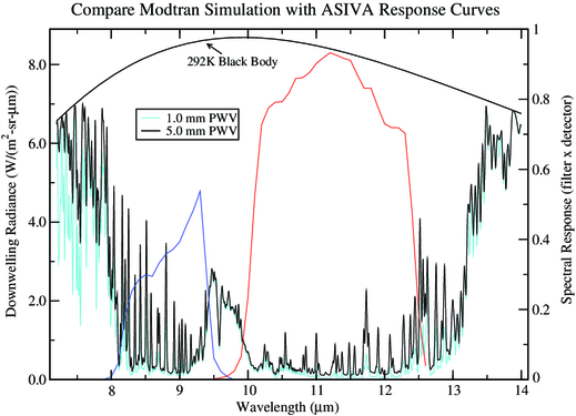
Fig. 1.— Simulated clear-sky downwelling spectral radiance for 1 and 5 mm PWV and filter response for two ASIVA filters (blue and red) used in this study.
This article will discuss the ASIVA instrument with particular emphasis on the novel calibration procedures that have been developed to improve mid-IR radiometric performance. Data presented here were gathered with the Large Synoptic Survey Telescope (LSST) project's ASIVA instrument. The LSST-ASIVA has been operationally tested on Kitt Peak, AZ and at the University of New Mexico's campus observatory located in Albuquerque, NM. Ultimately, the LSST-ASIVA will be permanently installed on Cerro Pachón in Chile where its objective will be to provide the LSST scheduler with real-time measured conditions of the sky/clouds, including high cirrus to better optimize the observing strategy. Data analysis procedures have precipitated the creation of a sky quality metric designed to quantify the photometric quality of the sky, which is presented in this article.
2. DESCRIPTION OF ASIVA INSTRUMENT
The ASIVA instrument has been described in detail elsewhere (Sebag et al. 2008, 2010). The IR camera subsystem features a 640 × 512 uncooled microbolometer array sensitive to 8–14 μm radiation, a 180-degree (all sky) custom designed hard carbon coated waterproof lens, and a six-position filter wheel. The IR camera provides image data at 14-bit resolution at a 30 Hz rate. Sixteen of these images are coadded to produce a single frame with an effective exposure time of 0.53 s. Up to eight of these frames are then bundled to produce a three-dimensional FITS file (data cube) that is stored to disk for further processing. The ASIVA instrument features a unique Hatch/Radiation Shield subsystem used for image calibration and protection from precipitation. This subsystem provides the following relevant features: (1) IR blackbody reference remains in the same protected orientation (pointed downward) as the hatch is opened and closed. (2) Temperature sensors and a heater are embedded in the IR blackbody reference for accurate in situ radiometric image calibration. (3) Radiation shield allows the blackbody reference to equilibrate with the ambient air temperature.
The LSST-ASIVA also features a high-sensitivity (but uncooled) 1392 × 1040 monochrome CCD camera coupled with an off-the-shelf 180-degree lens. The camera is fitted with a longpass filter (cutoff at 550 nm) and is capable of exposures of up to 2 minutes in length. The visible subsystem has been primarily used to show the advantages of using infrared over visible technology in the detection of thin clouds at night (Sebag et al. 2010). Radiometric calibration of the visible subsystem is the subject of future research. New ASIVA instruments are now being fabricated with a cooled 2048 × 2048 CCD camera coupled with a filter wheel for the purposes of conducting precision UBVRI photometry. A schematic of the LSST-ASIVA instrument is shown in Figure 2.
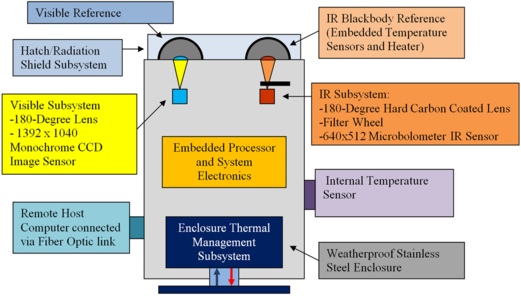
Fig. 2.— Functional schematic of the LSST-ASIVA instrument.
An acquisition script governs which data are acquired during an observing sequence. Each sequence begins with the hatch closed wherein IR blackbody reference images are acquired in each of the selected filters. The hatch is then opened and sky images are acquired until the next sequence begins (typically chosen to be a 5-minute interval). A process script analyzes the acquired images as is described in this article and creates a series of data products that are stored into a single web database, which can be used by observatory operations.
3. INFRARED RADIOMETRIC CALIBRATION
The ASIVA instrument incorporates a two-step calibration process in determining the spectral radiance for IR images. The first step is to determine the instrument response of the array and the second step is to perform a final calibration of the spectral radiance image based on analysis of the instantaneous observations. These steps are described in detail below.
3.1. Determination of Instrument Response Coefficients
The first step in this calibration procedure is to determine the instrument response coefficients Gλ for every pixel in the array in each filter. These coefficients are generated using equations (1) and (2).
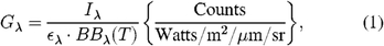
where Iλ = Instrumental Counts for the Blackbody reference in a specific filter,  λ = Emissivity of the Blackbody for a specific filter, and
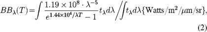
where tλ = system response as a function of wavelength for a specific filter.
The blackbody spectral density BBλ(T) above assumes a wavelength λ given in units of microns ( μm) and is averaged over the system response tλ (which includes the combined effect of filter/lens transmission and nominal IR detector sensitivity as a function of wavelength) for a particular temperature T in kelvin. The emissivity λ of the blackbody depends on the coating and design of the calibration reference used to cover the IR lens. The ASIVA reference has a series of ridges cut into it and was painted with an ultra-flat black paint. The emissivity is assumed to be constant for a given filter but can be adjusted from one filter to the next if necessary. As will be shown later in this section, the exact value of the emissivity is not particularly critical. A value of 0.98 was used throughout this study.
To eliminate instrumental offsets, Gλ is determined by calculating a least squares linear fit to the Iλ versus λ·BBλ(T) data for a range of temperatures T. The built-in blackbody reference located inside the hatch cover is used to determine the instrumental response of the system and also eliminate the fixed pattern components in the image during normal operation. Three temperature sensors are bonded within the blackbody reference near the emissive surface and the temperature data are written into the FITS header when acquiring images. A heater is also attached to the back surface of the blackbody to control its temperature during calibration.
During the calibration procedure, the hatch is opened and the blackbody is heated to ∼80°C. The blackbody is then allowed to cool passively to near ambient temperature. During the cool-down period, the hatch is periodically closed ( ∼5 minute intervals) to take calibration data in each of the desired filters. Data are acquired in this fashion for approximately 60 minutes wherein the hatch stays open for the majority of the time to prevent heating of the IR lens during the calibration procedure. The data is analyzed as described above and a calibration image file containing the Gλ values for each pixel is created. An example of a calibration data set used to establish the Gλ value for the central pixel in the 10.2–12.2 μm filter is provided in Figure 3. The response is very linear over this radiance range. We have found that Gλ does not vary significantly over time and therefore this calibration procedure need only be performed once or twice a year.
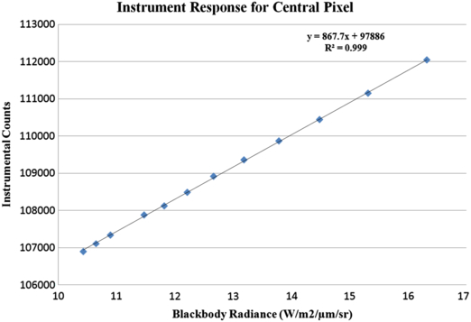
Fig. 3.— Instrument response versus integrated radiance for central pixel in 10.2–12.2 μm filter.
A primary advantage of ASIVA's up-looking lens is that it views the uniform blackbody reference through the same optical path in which it views the sky, thus eliminating any need to compensate for optical path differences. In addition, the calibration procedure accounts for differences in the solid angle per pixel, one of the attributes of a wide-angle lens. In general, the Gλ values are seen to be relatively constant over the field-of-view (FOV) as the reduced effective aperture is balanced by the increased solid angle as one moves from the center to the edge of the field.
Using the Gλ values established in the procedure discussed above, the spectral radiance ( Fλsky) of each individual observation is computed using equation (3):
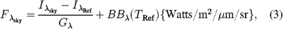
where Iλsky = Instrumental Counts measured for the sky image, IλRef = Instrumental Counts measured for the Reference Blackbody image, Gλ = Instrument response coefficients derived from equation (1), BBλ(TRef) = Integrated blackbody radiance derived from equation (2) for temperature TRef.
Here the blackbody reference temperature ( TRef) is that which is acquired at the time of the observation.
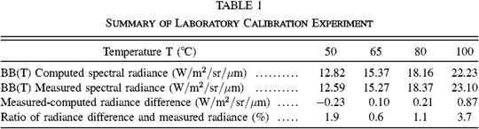
A commercial external blackbody was set up in the lab alongside the ASIVA instrument to verify this procedure (Sebag et al. 2010). The external blackbody was placed at a distance so that its circular aperture created a 10-pixel diameter spot on the focal plane. The external blackbody temperature was stepped between 50 and 100°C and a series of images were acquired. The spectral radiance of these images was computed according to equation (3) and the spectral radiance values within the 10-pixel diameter spot were compared to the spectral radiance values computed from the external blackbody temperature. The results for the 10.2–12.2 μm filter data are given in Table 1. Good agreement ( ∼1–2%) was obtained for temperatures between 50 and 80°C with a trend to larger errors as one departed further from the ambient radiance ( ∼9.0 W/m2/sr/μm). Possible sources of error for this trend include: errors in determining the instrument response coefficients, errors in the absolute temperature measurement of the blackbody reference temperature sensors, and a departure from sensor response linearity at higher temperatures.
 |
3.2. Calibration of Spectral Radiance Images
Our research has revealed that a second calibration step is required, as the laboratory experiment described above did not properly emulate typical observing conditions. In the lab, the radiation environment experienced by the imaging system was essentially identical whether the hatch was opened or closed, whereas during typical observing the infrared lens is exposed to clear transmitting sky when the hatch is opened. This causes the lens (more specifically its hard carbon coating) to radiatively cool when exposed to the sky and warm when exposed to the blackbody reference. This introduces a systematic offset in the IλSky - IλRef term in equation (3) that is not accounted for in the determination of the instrument response coefficients discussed in § 3.1. In general, errors in determining Fλsky are largest when observing clear-sky conditions where IλSky - IλRef is greatest and Fλsky is near zero radiance. This is the region for which the ASIVA instrument nominally operates and where the calibration is required to be most precise. To correct for any systematic offsets along with other possible errors that may creep into the calibration process, we introduce an offset term ΔOffset to equation (3) to represent all potential offsets. The novel calibration method we present here explains how the all-sky capability of the ASIVA instrument is invoked to yield additional information for determining the value of ΔOffset and therefore more accurately determine Fλsky. With this offset term, the sky's spectral radiance ( FλSky) for a given filter is determined using equation (4).
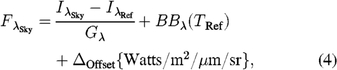
where ΔOffset = Potential offsets introduced in the calibration and observation procedure.
The ΔOffset term is subject to the instantaneous radiation environment at the moment of sky and reference image acquisition and therefore must be determined for every sky image. In general we expect to apply the largest offset correction during clear-sky conditions with low PWV levels where the downwelling radiance onto the lens is at a minimum when the hatch is open. The downwelling radiance is also subject to the zenith angle (i.e., airmass) and it is this fact that is exploited using ASIVA's all-sky capabilities to determine ΔOffset. A useful quantity in the analysis presented below is the normalized spectral radiance  given by equation (5). The dimensionless normalized spectral radiance can be thought of as a proxy to the sky's emissivity.
  is generally an underestimate of the true emissivity since the ambient temperature given by TRef is nominally greater than the mean temperature of the emitting sky.

A series of MODTRAN simulations were run to provide a parameterization of the normalized clear-sky downwelling radiance as a function of PWV and airmass. Simulations were run for a standard mid-latitude summer atmosphere at a base altitude of 2,400 m with zero haze and a nominal value for the lapse rate. Different PWV values were attained by adjusting the relative humidity, which was assumed to be constant as a function of altitude above the base. For each simulation the integrated normalized downwelling radiance was determined in each of ASIVA's filters. A second-order polynomial given by equation (6) was then used to fit the simulated data as a function of airmass for a variety of PWV values ranging from 0 to 24 mm.

The coefficients A0, A1 and A2 of equation (6) were then determined by their own second-order polynomial equation as a function of PWV as described by equations (7a), (7b), and (7c).


where HC10–12 μm = Multiplicative factor used to vary the amount of contributing Haze.
Note that the HC10–12 μm multiplicative term applies to the zero-order terms in equations (7a), (7b), and (7c) and therefore represents an adjustment of the PWV = 0.0 mm contribution to the normalized radiance. The results of this parameterization with no haze ( HC10–12 μm = 1.0) for selected values of PWV are shown in Figure 4. A similar parameterization was computed for the 8.25–9.25 μm filter. Additional MODTRAN simulations for PWV = 0.0 mm and varying visibility were run to establish the relationship between HC10–12 μm and HC8.25–9.25 μm yielding the surprisingly simple relation expressed in equation (8).

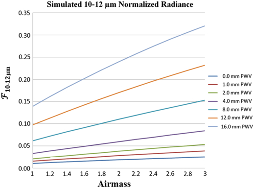
Fig. 4.— Simulated normalized clear-sky downwelling radiance as a function of airmass for selected values of PWV and no haze utilizing the 10.2–12.2 μm filter.
Therefore the haze correction is essentially common to both filter parameterizations and is not varied independently. The motivation for using normalized radiance was to produce a model that is largely insensitive to the ambient temperature. Future research investigations will vary the lapse rate as well as the water vapor profile in an effort to extend the model and quantify its robustness.
Results of from these simulations are then compared to  versus airmass data in order to determine the best possible fit as a function of PWV. This is accomplished by first binning the
  data into 29 airmass bins ranging from 1.0 to 3.0 airmasses. Each bin was selected to contain a similar number of pixels ( ∼6,000) in the IR array. This approach allows one to select the lower envelope of
  values and avoid contamination of the clear-sky data due to clouds and other obstructions in the field-of-view. This lower envelope is best fit to the overall shape (not the overall level) of the MODTRAN data described in equation (6) and the value for PWV is determined. Using this value of PWV one can then determine ΔOffset/BBλ(TRef) (i.e., the normalized offset) value, which is simply the constant offset between the observed and modeled data. At present we assume the offset to be independent of airmass; however, this may not be correct due to emissivity variations from the center to the edge of the lens. This possibility will be explored in future research.
A second-order polynomial is also fit to the lower envelope of data values (adjusted by ΔOffset/BBλ[TRef]) and serves as a model of the underlying clear-sky normalized radiance. Figures 5a and 5b show the results of this analysis for clear-sky conditions utilizing the 10.2–12.2 μm filter. The clear-sky envelope is clearly evident in Figure 5b with the data values departing from this lower envelope beginning at ∼1.8 airmasses corresponding to buildings and other obstructions in the field-of-view. The standard deviation of the normalized radiance in the 1.0 airmass bin is measured to be ∼0.004 and increases to ∼0.008 at 1.8 airmasses. This is a factor of 5–10 times greater than the measured sensitivity of the instrument suggesting that these variations are due to true normalized radiance variations in the airmass bins.

Fig. 5.— (a) 10.2–12.2 μm calibrated  image for clear-sky conditions acquired at the University of New Mexico's campus observatory on 2010, November 22. Image truncated at 6.0 airmasses. (b)
  vs. airmass plot for image shown in Fig. 5a. Red line indicates best fit MODTRAN model for PWV = 7.8 mm and gold plus symbols indicate average
  value in lower envelope ( ∼100 data points) in each airmass bin.
We have found that varying the HC10–12 μm factor (and therefore HC8.25–9.25 μm) described in equations (7a), (7b), and (7c) can be used to achieve consistency between the 10.2–12.2 μm and the 8.25–9.25 μm data. The data shown in Figure 5b as well as its companion data acquired in the 8.25–9.25 μm filter are best fit by a MODTRAN model with a PWV value of 7.8 mm and an HC10–12 μm factor of 2.62 ( ∼10 km visibility). Figure 6 shows the sensitivity of the fit in determining this PWV value from the 10.2–12.2 μm data. The best fit at 7.8 mm should not be interpreted as an absolute measure of PWV as further calibration of this technique is required. By using data from two filters, this analysis technique allows for both the determination of PWV and the contributing haze. As an independent verification of the PWV estimate, a value of 6.7 ± 1.5 mm was obtained for this time period using ground-based GPS meteorology analysis provided by NOAA's Earth System Research Laboratory. In the future we will be using independent PWV measurements such as these to further calibrate this technique.
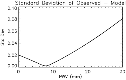
Fig. 6.— Standard deviation of the difference of the lower envelope of data points in each airmass bin compared with MODTRAN simulation data of varying PWV.
A value of ∼0.25 for ΔOffset/BBλ(TRef) is required for consistency between the model and measured data shown in Figure 5b. As discussed above, this positive offset value is consistent with the fact that the radiation environment onto the imaging system is significantly lower when viewing the sky as opposed to viewing the reference blackbody. Note that without this offset, unphysical negative radiance values would result. Also note that with this offset, normalized radiance values of the obstructing buildings are near 1.0, consistent with the fact that they are at or above ambient temperature. Future observations will utilize a blackbody source placed in the FOV to help verify the calibration procedures discussed in this section.
Figures 7a and 7b show the results of a similar analysis for cloudy sky conditions. The clear-sky envelope is still clearly evident in Figure 7b. As can be seen by the lower envelope of data values in each airmass bin, this methodology is very robust to the presence of clouds and other obstructions.
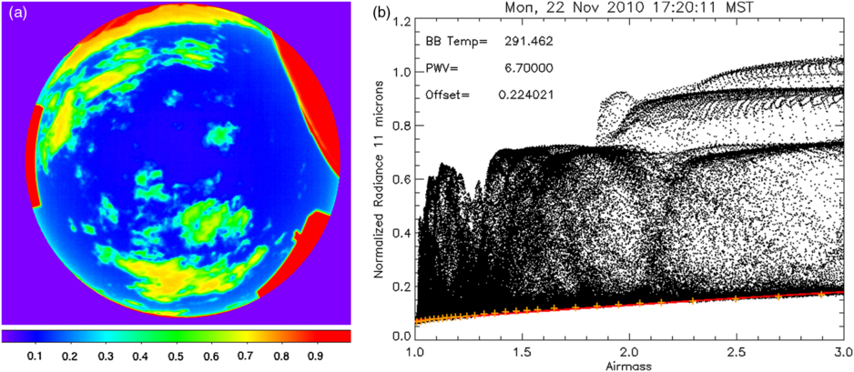
Fig. 7.— (a) 10.2–12.2 μm calibrated  image for cloudy-sky conditions acquired at the University of New Mexico's campus observatory on 2010, November 22. (b)
  vs. airmass plot for image shown in Fig. 7a. Red line indicates best fit MODTRAN model for PWV = 6.7 mm and gold plus symbols indicate average
  value in lower envelope ( ∼100 data points) in each airmass bin.
4. CLOUD DETECTION AND SKY QUALITY
Three data products are currently generated from the radiance-calibrated and raw images to determine the presence of clouds and the photometric sky quality. The first of these data products is referred to as the temporal standard deviation image. This image is generated by computing the standard deviation of the eight individual images stored in the data cube. The second data product is referred to as the spatial standard deviation image. This image is generated by computing the difference between the first and last image in the data cube and then replacing each pixel value with the standard deviation of pixel values within a box centered on that pixel. Finally, a clear-sky subtracted image is generated by subtracting the clear-sky normalized radiance determined by the fit to the lower envelope of  values in each of the airmass bins from the calibrated normalized radiance image. Note that the clear-sky subtracted image is independent of the MODTRAN simulations and analysis discussed above. Figures 8a, 8b, and 8c show the resulting images from this analysis using the data presented in Figure 7b.
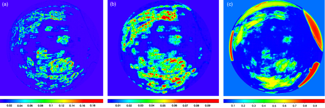
Fig. 8.— (a) Temporal standard deviation image generated from data presented in Fig. 7. (b) Spatial standard deviation image. (c) Clear-sky subtracted normalized radiance image.
Though there is considerable overlap, the images shown in Figures 8a, 8b, and 8c are also complimentary. These data products are therefore combined with different weighting factors to produce a single metric image characterizing the photometric quality of the sky on a scale of zero to one. The sky quality map is also smoothed which essentially extends the boundaries of cloud structures. In practice, this will help avoid the selection of photometric skies that are too close to those that are not. Results of this analysis are shown in Figure 9.
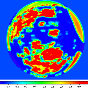
Fig. 9.— Sky quality map generated from data presented in Fig. 7.
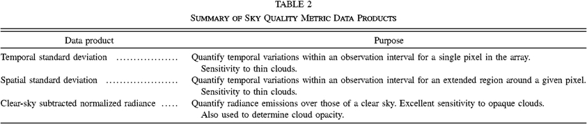
The clear-sky subtracted image is given a weighting factor of unity and therefore reveals variations in the sky's emissivity. However, as mentioned above, some variability is expected due to variations in temperature and PWV at a given airmass. To distinguish the presence of thin clouds the temporal and spatial standard deviation images are utilized. These images are given appropriate weighting factors to bring their clear-sky variability on par with that of the clear-sky subtracted image. In Figure 9, photometric conditions are seen to lie in the 0.02–0.03 range on this scale. Refining and interpreting this metric is the subject of ongoing research. Table 2 provides a summary of the data products that go into the sky quality metric. This metric can ultimately be used by the observatory scheduler to make appropriate telescopic observation decisions.
 |
5. CLOUD TEMPERATURE DETERMINATION
Two cloud temperature data products can be derived from spectral radiance calibrated images. The brightness temperature of the sky ( TλBrightness) for a given filter can be determined by equating the sky's spectral radiance ( FλSky) with a blackbody whose temperature yields this same spectral radiance. For clouds that are optically thick, TλBrightness yields a temperature close to that of the cloud base. The color temperature of the sky ( TColor) can be inferred by taking the ratio of the sky spectral radiance acquired in the 8.25–9.25 μm and 10.2–12.2 μm filters and equating this to the blackbody radiance ratio of these two filters at temperature Tcolor Color temperature has the distinct advantage of being largely indifferent to the optical depth of the cloud and therefore can yield a better measure of the true temperature for clouds. Both temperature measurements are subject to dilution by the clear-sky emission along the path. Results of this temperature analysis are shown in Figures 10a and 10b. Temperature values are reported only for pixels whose normalized radiance is greater than 0.03 above the clear-sky normalized radiance.
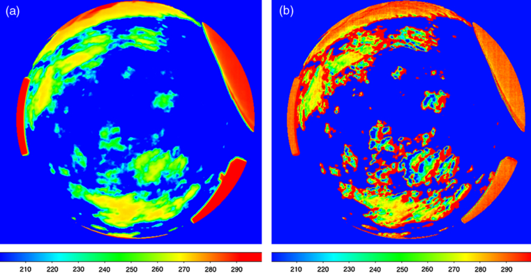
Fig. 10.— (a) Brightness temperature (K) image generated from data presented in Fig. 7. (b) Color temperature (K) image.
Both images in Figure 10 show similar temperatures in the optically thick regions of the clouds. As expected, the TλBrightness image shows lower temperatures at the periphery of clouds due to the lower optical depth there. The TColor image is much more varied due to the motion of the clouds over the data acquisition period but is essentially uniform across the cloud. In future research we will investigate summing over the radiance of cloud structures to obtain a more accurate measure of TColor. In addition, sky images in the 8.25–9.25 μm and 10.2–12.2 μm filters will be acquired at a faster cadence to reduce cloud motion between the acquisition of each image. Using the cloud temperature as determined from TColor, the optical depth of a cloud can be determined by comparing the radiance of the cloud with that of a blackbody at TColor. Ultimately the goal is to compare this optical depth with the extinction in the optical spectrum. This is a subject of ongoing research.
6. SUMMARY
In this article we have discussed a novel radiometric calibration and data analysis procedure for the ASIVA instrument. The analysis appears to be very robust and allows for the determination of several key data products relevant to ground-based astronomical telescopes. Most importantly this analysis allows for the determination of a sky quality image that can serve as a consistent and reliable metric for telescope scheduling purposes. Future research will concentrate on correlating the infrared data with the extinction found in the visible spectrum.