

ABSTRACT
The quality of astronomical images obtained with the 3 m liquid‐mirror telescope (LMT) of the NASA Orbital Debris Observatory (NODO) and with the University of British Columbia 6 m Large Zenith Telescope (LZT) is assessed and compared to that of conventional instruments. Analysis of star images in long‐exposure drift‐scan data indicates that the profile of the image core is primarily set by atmospheric turbulence. Defocused star images reveal the presence of low‐amplitude waves on the surface of the mercury, also seen in laboratory tests. The effect of these waves is to diffract light into the wings of the point‐spread function. Analysis of the intensity profiles of stellar images can therefore probe the structure of the mirror surface on scales smaller than the atmospheric coherence length, which is about an order of magnitude larger that the characteristic wavelengths of the surface waves. It is found that the rms surface height error produced by these waves was approximately 37 nm for the NODO LMT. Improvements to the rotational speed stability of liquid mirrors, reduction of the thickness of the mercury layer, and use of a protective Mylar cover have allowed the LZT to reduce this source of error to approximately 9 nm rms, thereby achieving an image quality approaching that of conventional telescopes.
Export citation and abstract BibTeX RIS
1. INTRODUCTION
Over the past decade, LMTs (Borra 1982) have come into use in astronomy, space research, and atmospheric physics (Hickson et al. 1994; Sica et al. 1995; Potter & Mulrooney 1997; Wuerker 2002). One of these, the 3 m LMT of the NODO (Potter & Mulrooney 1997; Mulrooney 2000), was built to study space debris during times near twilight. This instrument has also been used to conduct a series of drift‐scan astronomical observations using a set of narrow and broadband filters (Hickson & Mulrooney 1998). Recently, a 6 m astronomical LMT, the LZT (Hickson et al. 1998, 2006), has seen first light. The success of these telescopes has spurred interest in the possibility of employing liquid mirrors in future very large telescopes (Hickson & Lanzetta 2003, 2004).
The principal attraction of LMTs is their relatively low cost: liquid mirrors in the 3–6 m range cost approximately $10,000 per square meter, about an order of magnitude less than glass mirrors. For survey‐type programs in which the restriction to near‐zenith pointing is not a significant limitation, dedicated LMTs can provide new research opportunities.
The optical properties of rotating mercury mirrors have been studied extensively in the laboratory (Borra et al. 1985a, 1985b, 1989, 1992, 1993). Interferometric tests reveal these mirrors to have a parabolic surface, accurate to within a fraction of a wavelength. Surface waves on the mercury, produced by vibration and wind, are evident in these tests. The amplitude of these waves depends on the level of disturbance and the thickness of the mercury layer (Girard & Borra 1997; Tremblay & Borra 2000).
The performance of liquid mirrors under actual observing conditions is less well documented. It is reasonable to ask whether a rotating mercury mirror—when exposed to wind, temperature extremes, humidity, dust, vibration, etc.—can perform as well as one in a controlled laboratory environment. The ultimate test of any telescope is of course its ability to deliver scientifically useful data.
Laboratory mirrors can be tested directly by interferometric techniques that illuminate the mirror from, and analyze images at, their center of curvature. However, it is rarely the case that the center of curvature is accessible in an astronomical telescope. Furthermore, the use of stars as reference sources is problematic with telescopes that do not point and track. Because of this, the characterization of LMTs must necessarily rely on less direct methods. One of these methods is the quantitative analysis of intensity profiles of star images obtained by drift‐scan observations. This type of analysis is particularly useful in assessing the optical quality of the liquid‐mirror surface on small scales: those less than the atmospheric coherence length. These are precisely the scales that are of the most importance in telescopes that employ adaptive optics to reduce the effects of atmospheric seeing.
2. DATA
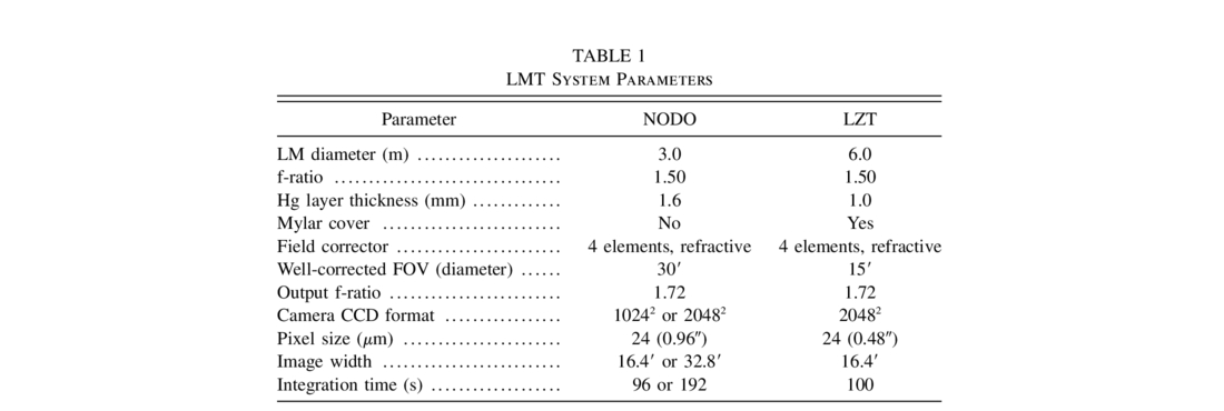
The primary data for this analysis consist of drift‐scan observations obtained with the NODO LMT and the LZT. Some details of the design and construction techniques employed for these liquid mirrors are given by Hickson et al. (1993). The LZT is described in detail by Hickson et al. (2007). Broadband interference filters were employed, giving passbands roughly equivalent to the Johnson R and I band. The parameters of the systems are given in Table 1. Of particular note is the sheet of 12 μm thick Mylar stretched over the mercury container of the LZT to protect it from contamination (insects, mostly) and to eliminate rotation‐induced wind over the fragile optical surface. The benefits from this measure are discussed below.
 |
The refractive prime‐focus correctors, designed by E. H. Richardson, provide well‐corrected images with very low distortion, as required for drift‐scan imaging. The CCDs are thinned back‐illuminated devices produced by SITe and integrated by PixelVision, Inc. The CCDs were oriented with their columns in the east‐west direction and operated in time‐delay integration (TDI) mode at the sidereal rate for the declination of the zenith. Data were recorded line by line, using Hickson's TDI software, then preprocessed and assembled into 1024 × 1024 or 2048 × 2048 pixel images for further analysis.
An image of a star field at mid‐Galactic latitude, obtained with the LZT, is shown in Figure 1. This field was selected for its saturated star images that allow the diffuse halo to be seen. A faint diffraction ring may be seen that arises from concentric waves at the edge of the mirror. An image of a high‐Galactic‐latitude field is displayed in Hickson et al. (2007).
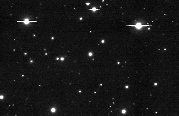
Fig. 1.— Image of a star field obtained in the R band with the LZT. The picture covers an area of 10' × 7' and has an integration time of 100 s. The image contains several heavily saturated stars (the horizontal lines result from charge bleeding along the columns of the CCD), for which the faint halo is just visible. Most of the faint objects seen in this field are galaxies.
At the NODO LMT, a second camera was used to obtain defocused images of bright stars in order to provide qualitative information about the liquid‐mirror surface. This camera employs a commercial video camera optically coupled to a microchannel intensifier. It was the primary camera used by NASA for space debris observations. When not in use, the camera was offset from the telescope axis and would occasionally record highly defocused images of bright stars that happen to illuminate it. An image from this camera is shown in Figure 2. It clearly reveals waves propagating on the mercury surface. Such waves have also been detected and studied in the laboratory tests of liquid mirrors cited earlier. Two types of waves are present: concentric waves created by vibrations propagate inward from the outer rim of the mirror, and less regular "spiral" waves are likely caused by rotation‐induced vortices in the air above the mirror, imprinting themselves on the mercury surface. Of particular interest is the characteristic wavelength, which ranges from ∼1 cm for the concentric waves to ∼5 cm for the spiral waves.
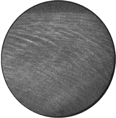
Fig. 2.— Portion of a defocused stellar image from the NODO LMT. Waves propagating on the mercury surface are clearly visible. These waves diffract light, forming diffuse halos around bright stars (courtesy M. Mulrooney).
To provide a comparison for the LMT data, representative images obtained with the MDM 2.4 m and Mayall 4 m telescopes were kindly provided by Arlin Crotts, and with the Palomar Hale 5 m telescope by Brett Gladman. Images from the Blanco 4 m telescope were obtained from the NOAO Web site.
3. ANALYSIS AND RESULTS
Composite intensity profiles were generated from isolated stellar images seen in the drift‐scan data. For each star, the fluxes in a series of concentric rings were computed. The radial increment for these rings was 1.0 pixel, and the rings were centered on the centroid of the image core. For each ring, the median value of the intensities of pixels whose centers fell on or within the circular region bounded by the ring—but outside that of the previous, smaller ring—was determined. The median value was used, as it is insensitive to the presence of other faint stars that would otherwise contaminate the intensity profile. The outer regions of the composite profile were determined from bright stars whose inner regions were necessarily saturated. The inner regions were determined from fainter, unsaturated star images. Profiles obtained from different stars were scaled in order to minimize the squared intensity differences in the overlap region.
The profile samples for each LMT camera system were made sufficiently large to ensure robust statistics for the resulting image quality parameters. A total of 121 profiles obtained over 25 nights spread over 13 months between 1999 and 2006 were thus examined.
The resulting profiles cover typically 5 orders of magnitude in intensity and extend to radii of 1.5'. The outer portions are particularly well defined, thanks to the relative ease of flat‐field calibration and sky subtraction of drift‐scan data. The inner portion of the NODO point‐spread functions (PSFs) lacks resolution because of the relatively large (0.96'') pixel size. It is, however, quite adequate for our purposes.
Data from the LZT were divided into three groups: 2004 semester 2 (04S2), 2005 semester 1 (05S1) and 2005 semester 2 (05S2). This allows us to track the performance from the commissioning to operations phase, during which engineering tests were carried out and refinements made.
In Figure 3 we show a comparison of model fits to the PSFs of the 3 m NODO LMT, the 6 m LZT, and a composite PSF derived from stellar profiles measured on images taken with the MDM, Mayall, Blanco, and Hale telescopes. In order to compensate for differences in atmospheric seeing, the atmospheric (Kolmogorov) component has been scaled to a common FWHM of 1.4'', the mean FWHM of the conventional telescope PSFs. In order to do this, it was first necessary to resolve the profiles into atmospheric and diffraction components as described in § 3.1. The LMTs show an excess intensity above the Kolmogorov profile that becomes apparent at a radius of approximately 3'' and drops off roughly as r-3. The conventional telescopes also show an excess intensity beginning at about the same radius, but at a lower level. Because of this, stars seen in images from LMTs have more noticeable halos than do those seen in images from conventional telescopes.
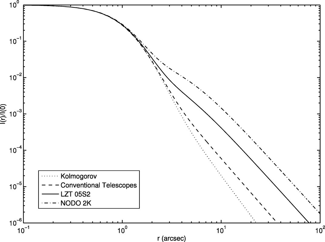
Fig. 3.— Comparison of stellar intensity profile fits derived from images with LMTs and conventional telescopes. The solid curve shows the PSF of the 6 m LZT, derived from drift‐scan images obtained in 2005 October. The dashed curve shows a composite of PSFs from the MDM 2.5 m telescope, the Mayall and Blanco 4 m telescopes, and the Hale 5 m telescope. For comparison, the dotted curve is the atmospheric Kolmogorov profile. To compensate for variations in seeing, the Kolmogorov component (only) of the PSFs has been normalized to a common FWHM of 1.4'' (the mean FWHM of the conventional telescope PSFs).
The presence of diffuse light over and above the seeing profile in these images is an important issue. It means that light has been removed from the core of the image, thus reducing the sensitivity and increasing the background light in crowded fields. Our aim is to determine the fraction of light that is scattered or diffracted into these halos, both for LMTs and for conventional telescopes, and thereby assess the relative performance. To do this requires a quantitative analysis of the PSF, which we now discuss.
3.1. Point‐Spread Function
We chose to model these PSFs as the sum of a Kolmogorov‐seeing disk and of a diffraction halo convolved with pixel sampling. Following Racine (1996), we used a convenient analytical model composed of Moffat (1969) functions whose form is
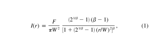
where F is the flux, W the HWHM, and β an index that controls the shape at large radii.
For a Kolmogorov profile falling off as r-11/3 in intensity at large r (Roddier 1981), β = 11/6. We established by numerical experiments that the seeing profile can be represented to accuracy better than 1% at all r by the sum of two Moffat functions having the same W = WK, and β = 4 and 11/6, respectively, with the core term containing 82.2% of the total flux.
The diffraction halo is represented by a Moffat function having β = 3/2, since it falls off with a power law of index −3. Indeed, for circular features such as the concentric waves, the Fraunhoffer diffraction kernel is the Bessel function J0(kr) whose integral over any finite radial interval falls asymptotically as r-3/2. Therefore, the diffraction pattern of random, circularly symmetric features falls asymptotically as r-3. For linear features, the diffracted intensity falls as r-2 in the direction orthogonal to the feature. Averaging over all angles, performed by the rotation of the mirror, changes the depencence to r-3.
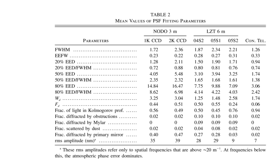
For each profile, the fitting algorithm iteratively minimizes the χ2 of the residuals by adjusting the relative fluxes and the widths of the seeing and diffraction profiles. The Kolmogorov+diffraction model fits the data very well, with typical errors less than 2%. The output from the algorithm also includes the FWHM of the resulting composite profile; the encircled fractional energy within that width (EEFW); the encircled energy diameters that contain 20%, 50%, and 80% of the total flux; the width Wd of the diffraction profile; and the fraction Fd of the total flux scattered in the diffraction halo. The results of the fits for all profiles are given in Table 2 and analyzed in § 3.1. Histograms for various PSF parameters are displayed in Figure 4.
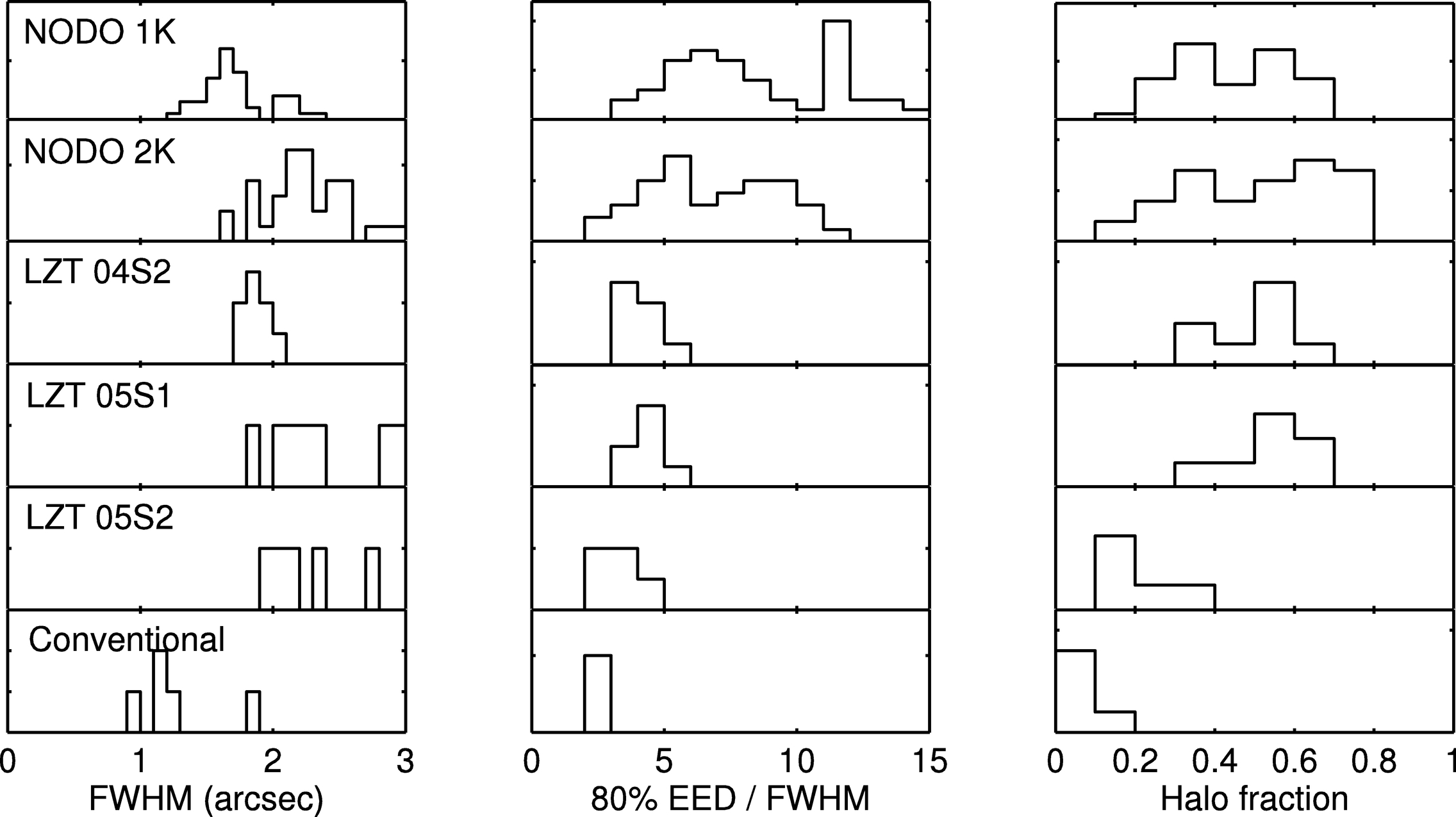
Fig. 4.— Statistics of PSF parameters for different data subsets.
 |
Several components of image degradation have been ignored in the analysis that follows. Drift‐scanned images suffer a degree of blurring due to star‐trail curvature and variation of the sidereal rate with declination. For a square or circular detector, the resulting image blur increases in proportion to the square of the angular field of view. It can be effectively eliminated by an appropriate corrector (Hickson & Richardson 1998), but such a corrector was not available. For the relatively small field of view (FOV) of the NODO 1K detector and of the LZT (16' × 16'), the rms contribution to image blur is only ∼0.3'', considerably less than the atmospheric seeing. For the NODO 2K FOV (33' × 33'), the effect is more severe and contributes to the systematically larger FWHMs obtained with this system, as shown below.
A further component of image blur results from the discrete nature of the shifting of charge in the CCD (Gibson & Hickson 1992). The images drift at a constant speed, but the electrons in the CCD are shuffled in discrete steps. This produces a rms image spread of 2/ 3 pixels (∼0.27'') in the east‐west direction. This also is ignored in the analysis.
3.2. PSF Parameters
A useful measure of image quality is the encircled energy–diameter (EED) relation. Figure 5 shows, for the various data subsets, the fraction of light from the star contained within a circle, centered on the star image, as a function of the diameter of the circle measured in FWHM. The EED relation for a pure Kolmogorov‐seeing disk is shown for comparison.
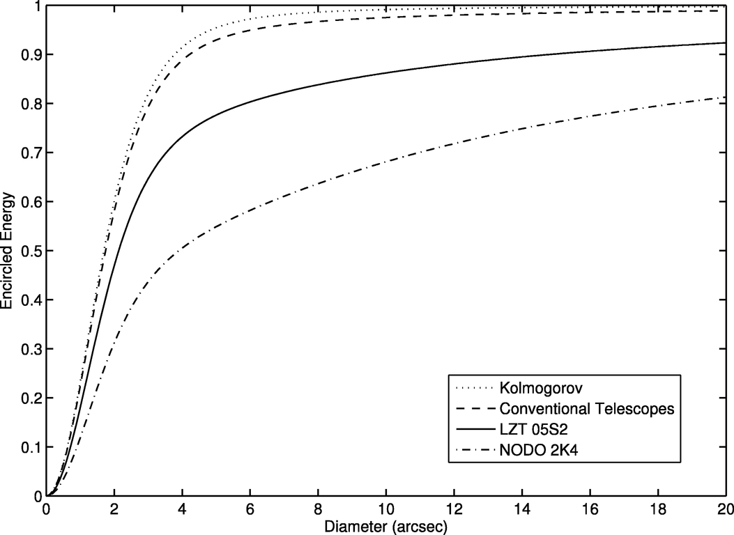
Fig. 5.— Encircled energy relations. The curves show, for the identified data subsets, the fraction of the total energy that is contained within a circle of specified diameter, centered on the star image. As in Fig. 3, the Kolmogorov component has been scaled to a common FWHM of 1.4''.
For the NODO LMT PSF, the encircled energy within a 2 × FWHM diameter circle is ∼50%, or 2/3 that for a Kolmogorov‐seeing disk. One‐third of the light reflected by the liquid mirror is scattered in a diffraction halo of FWHM∼6'' and a full width containing half the total power (FWHP) of 14''. With a high‐order adaptive optics system, a Strehl ratio of ∼0.65 in R would be possible.
The 1K and 2K NODO cameras yield similar EED relations. The image core is slightly broader with the 2K camera, probably because of the stronger aberrations in the outer regions of the wider FOV. The NODO images have a significant halo. This is in part due to atmopsheric seeing and scattering by dust and other small particles. However, the bulk of this light is due to diffraction from waves on the mercury surface, as is demonstrated in § 3.3.
For the LZT PSFs, the encircled energy within a 2 × FWHM diameter is ∼60%, or 3/4 that for a Kolmogorov‐seeing disk. One‐quarter of the light is scattered in a diffraction halo of FWHM 4'' and FWHP 9''. The LZT yields significantly better image quality than the NODO LMT while being of much larger aperture. This important finding is discussed further, after the analysis of the mirror structure functions in § 3.3.
In order to assess the performance of the liquid mirror, one must take into account other factors that contribute to diffraction or scattering out of the Kolmogorov component of the PSF. These include diffraction by obstructions, scattering by dust on the optical surfaces, and diffraction due to imperfections in other optical elements (such as the Mylar cover). Obstructions in the beam diffract an amount of light equal to the fraction of light obscured. Narrow objects diffract light to large angles. For wider objects such as the LZT hexapod legs, much of the diffracted light remains near the image core. Dust scatters light to large angles, effectively removing it from the image core. Imperfections in the LZT Mylar cover introduce an rms path error of 30 nm on scales of order 1 cm. The fraction of light diffracted out of the Kolmogorov component by such errors is 1 - exp (- k2σ2w)≃k2σ2w, where k = 2π/λ and σw is the rms wave‐front error. Thus, in the R band, the Mylar diffracts approximately 9% of the light to angles of order 10'' or more. To determine the performance of the liquid mirrors, one should first subtract these other components. What remains is then due to waves on the mirror. In Table 2, we estimate the contributions to the diffracted/scattered light for these other factors, and the resulting rms surface wave amplitude.
3.3. Structure Function
A complementary quantitative assessment of the quality of liquid mirrors and of the contributions to image degradation from atmospheric seeing and diffraction is the analysis of structure functions. In this section, we develop and apply the analysis to data from the NODO telescope. This telescope has no Mylar cover, so the images are affected by surface waves induced by vortices in the turbulent boundary layer above the mercury surface. The statistical properties of these waves can be investigated by examining the structure functions.
The phase structure function  ϕ(r) is defined to be the ensemble average of the squared phase difference between two points on the wave front separated by the two‐dimensional vector r (referred to the entrance pupil of the telescope),
In most cases, the structure function is isotropic and depends only on the scalar separation r = |r|.
The PSF is directly related to the structure function. For a long‐exposure image (i.e., averaged over atmospheric phase fluctuations), the modulation transfer function (MTF) is given by
where = ϕ + χ is the total structure function, the sum of phase and log amplitude fluctuations caused by scintillation (Fried 1966). For a large astronomical telescope, the latter is negligible (Hickson 1994). Hence,

Now, from Fourier optics theory, the MTF is proportional to the two‐dimensional Fourier transform of the PSF. For the case of circular symmetry, we have
where k = 2π/λ is the wavenumber. Therefore, one can determine the MTF and the structure function from the PSF.
The structure functions that describe various contributions to image degradation add to form the total structure function of the system. To see this, recall that independent effects, such as seeing and diffraction, all contribute in the form of convolutions applied to the PSF. By the Fourier convolution theorem, the MTFs of the various effects are therefore multiplied to obtain the system MTF. The additive property of structure functions then follows from equation (3).
For an LMT, the important contributions to image degradation are atmospheric seeing, diffraction by the aperture and obstructions, imperfections of the liquid mirror (LM), optical aberrations produced by the corrector, misalignment and defocus, and image spread due to the finite size of the CCD pixels.1 We proceed by quantifying all these effects, except that of the liquid mirror, and determining their contribution to the measured structure functions. In this way, we can determine the structure function of the LM alone. Once the LM structure function has been determined, one can readily predict the performance of the telescopes under other conditions, including the use of adaptive optics to compensate for atmospheric seeing.
The observed structure function is analyzed by first subtracting the structure functions due to diffraction and the finite pixel size (determined from the known MTFs using eq. [4]). What remains is a combination of the atmospheric structure function and that of the LM. The decomposition of these two is not unique. However, we are aided by the fact that structure functions must increase monotonically or remain constant. Furthermore, the structure function is related to the covariance function ℬϕ(r) = 〈ϕ(x)ϕ(x + r)〉. From the definition (eq. [2]), it is evident that
This shows that for disturbances that are uncorrelated on large scales, the structure function approaches the constant value 2ℬϕ(0). Disturbances on the mercury surface should be uncorrelated over distances much greater than their wavelength, so we expect a flattening of the LM structure function. Finally, we have some prior knowledge of the atmospheric structure function. Assuming Kolmogorov turbulence, it is given by
The Fried parameter r0 (Fried 1966) can be estimated from the FWHMs of the PSF. In fact, the main result of the analysis, the surface height variance, is not strongly affected by the choice of r0.
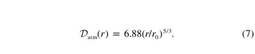
The results of the analysis are shown in Figure 6, in which the total structure function and its constituent parts are plotted. As expected, the LM structure function flattens. It can be fit quite well by the simple two‐parameter relation
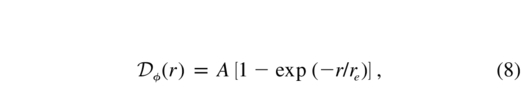
where A = 4.1 and re = 0.028 m. Since the phase error φ produced by fluctuations of height z on the mirror is 2kz, the rms surface height error is σz = A1/2/25/2k = 36 nm. This agrees very well with the results in Table 2, obtained by the PSF fitting method. Equation (8) indicates that unprotected LMs have a covariance that drops exponentially with distance, with a scale length of approximately 3 cm—a distance comparable to the observed wavelength of vortex‐induced spiral waves on the mercury. We discuss the implications of these results, and ways in which the performance of LMs can be improved, in § 4.
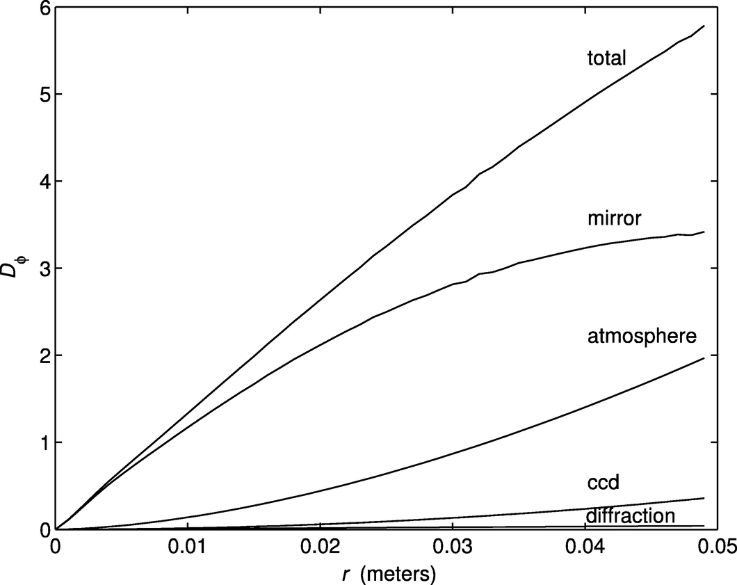
Fig. 6.— Structure functions and their components. The upper curves are the structure functions derived from the median stellar profiles for each data subset. The lower curves show the contributions due to diffraction. The curve marked "atmosphere" assumes a Kolmogorov turbulence spectrum and a Fried parameter calculated from the seeing FWHM. What remains after subtracting these components from the total is shown by the curves labeled "mirror," representing the contribution from disturbances on the liquid primary mirrors.
4. DISCUSSION
The principal conclusion of this study is that astronomical liquid‐mirror telescopes can and do provide images of scientific quality. These images are much like those produced by conventional telescopes. Like for other telescopes, the images have a core, with resolution limited by atmospheric seeing, and a halo. The main difference between the images produced by existing astronomical LMTs and conventional telescopes is that the halo contains a contribution produced by light diffracted from waves on the mercury surface.
How can we be sure that the resolution of these images is in fact limited by atmospheric seeing and not by some other effect? Misalignment of the rotation axis can give rise to long‐wavelength waves on the mirror (Borra et al. 1992). The Coriolis acceleration due to the Earth's rotation can have the same effect. However, both can be completely eliminated by proper alignment of the rotation axis: a small axis tilt serves to completely cancel the Coriolis effect (Hickson 2001, 2006). Any wobble of the axis would result in periodic motion of the star images. Such a wobble is evident for mechanical bearings due to coning error (Tremblay & Borra 2000), but is negligible for air bearings (Girard & Borra 1997). With the NODO telescope, wobble can be induced by mirror imbalance. This results from flexure of the air‐bearing support system and telescope pier. This wobble can be, and has been, eliminated by proper balancing of the mirror. The NODO mirror was balanced by adding small weights to the perimeter and observing the effects on star trails. Such images are easily generated by setting the CCD scan rate lower than the sidereal rate. Any wobble manifests itself as periodic oscillations in the trailed stellar images. These were evident before balancing but were removed with the correct position and weight of the balance mass. This was done once, and it has not been necessary to rebalance.
Figure 7 shows transverse position as a function of time, measured from a star trail. For clarity, the plot has been smoothed with a boxcar filter of width 0.1 s. The random fluctuations that can be seen are consistent with atmospheric seeing. The tip‐tilt components of seeing, which contain most of the phase variance, produce excursions in the image position both perpendicular and parallel to the direction of the trail. The former causes transverse excursions of the star trails; the latter causes variations in apparent intensity. What is significant in these images is the absence of any periodic component that would arise from errors in the mirror alignment or balance, or coning error of the bearing. Such effects would have an 8.5 s period, corresponding to the rotation of the mirror.
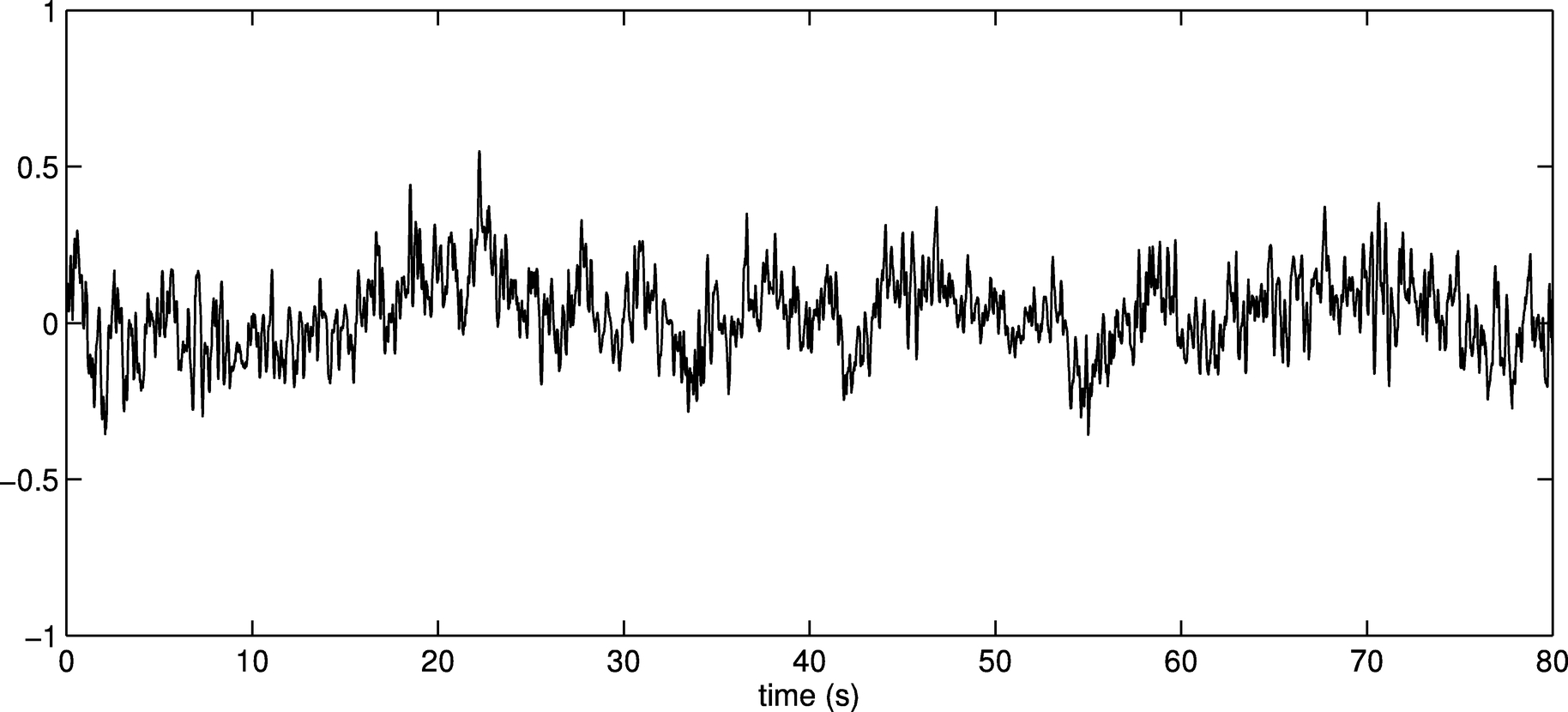
Fig. 7.— Transverse position of the centroid of a star trail, smoothed over a 0.1 s time interval, plotted vs. time. The random motion is consistent with atmospheric seeing. The rotation period of the LM is 8.5 s. There is no evidence of any periodic motion that might arise from errors in the primary mirror alignment or balance.
The rms transverse image displacement for the (unsmoothed) star trail is σα = 0.31'', and the mean FWHM is ε = 1.638''. For Kolmogorov turbulence, these two parameters are related by
and
(Sarazin & Roddier 1990); hence
If the image motion is due entirely to atmospheric seeing, the image FWHM predicted by equation (11) would be 1.42''. This is only slightly smaller than the measured FWHM. The small difference could easily be due to a focus error. This supports the conclusion reached in § 3 that the dominant cause of blur in the image core is atmospheric seeing.
Can the performance of liquid mirrors be improved further? It has been convincingly demonstrated in laboratory tests that a good way to reduce the amplitude of the surface waves, and thereby reduce the amount of light in the halo, is to make the mercury layer as thin as possible (Girard & Borra 1997; Tremblay & Borra 2000). These tests show a dramatic decrease in wave amplitude and improvement in surface quality as the mercury thickness is reduced from 2.8 to 0.8 mm. The thickness of the mercury film on the NODO mirror was 1.6 mm. It was not possible to easily reduce it, as the telescope had no provision for pumping mercury from the mirror while it was rotating. The mirror could not be started with a thin layer because the high surface tension of mercury prevented it from covering the mirror surface. New LMTs, such as the 6 m LZT and others being planned, include a system for pumping the mercury down to a thickness of 1 mm or less.
A second factor affecting LM image quality is rotational speed stability. All LMs to date, with the exception of the LZT, are run with open‐loop speed control. The NODO telescope, for example, used a three‐phase brushless DC motor integrated into the air bearing. An oscillator and linear amplifier providing current to the field windings generated a magnetic field that rotated at the desired rotation speed of the mirror. The permanent‐magnet rotor of the motor rides in the potential wells of this field, turning the mirror at the same average speed. Such a system is quite sensitive to disturbances, caused primarily by wind.
For the NODO telescope, period fluctuations of several parts per million (ppm) were observed in stable air with the dome closed. With the dome open, fluctuations increase from approximately 10 ppm with no wind to as much as 100 ppm in strong winds. Such fluctuations inevitably disturb the equilibrium of the mercury film, degrading the image quality. One can obtain a rough estimate of the magnitude of the effect by noting that a 10 ppm change in angular rate would, over several rotation periods, result in a 20 ppm change in focal length. This would produce about 90 μm of defocus and an image blur diameter of 60 μm (2.4'') with the NODO telescope. There is a clear correlation between mirror period fluctuations and image FWHM. Typically, the FWHM increases from approximately 1.6'' to 2.3'' as the fluctuations increase from 10 to 25 ppm (Mulrooney 2000).
This problem has been successfully addressed with the LZT. For this telescope, the mirror rotation period can be determined very precisely by gating a stable high‐resolution frequency counter by a once‐per‐revolution encoder index pulse. (This technique avoids all errors due to encoder nonconcentricity or optical mask inaccuracy.) The 6 m primary mirror of this telescope is not well protected from the wind, and period fluctuations as high as 1000 ppm were observed with open‐loop operation, even in light wind. The telescope now employs a closed‐loop servo control system that achieves 1 ppm period stability under all conditions.
The LZT has also achieved thin layers. It operates with a stable mercury film of ∼1 mm thickness. Even so, waves induced by the spiral vortices were clearly visible to the eye. These surface waves diffracted much light into the halo of the PSF. This problem was solved by the installation of a Mylar cover (Hickson et al. 2007). This cover consists of Mylar sheets held in a frame that is attached to the mirror and rotates with it. Once this cover was installed, the waves dissapeared.
The LZT's Mylar cover is effective at eliminating rotation‐induced waves, but the present 12 μm Mylar introduces significant phase errors. Mylar film is available as thin as 1.4 μm. Samples of the 12 and 1.4 μm film have been measured interferometrically (B. Truax 2006, private communication), and the latter was found to have a rms optical path error of 0.006 waves, 6 times smaller than the 12 μm material. This thinner Mylar would diffract a negligible amount of light, so there are plans to install it on the LZT, replacing the thicker Mylar currently in use.
It is clear from Figures 3 and 4 that much progress was made with the LZT during the engineering phase. The best results are from the most recent data (05S2), which were taken over a period of 3 months after improvements were made to the alignment of the mirror, and shortly after the Mylar surface had been cleaned for the first time since its installation more than a year earlier. Tests conducted at the United Kingdom Infrared Telescope (UKIRT) for the Gemini Project indicate that a horizontal surface in a typical observatory environment accumulates dust at a rate of 0.0011% hr−1. This corresponds to ∼5% coverage after 6 months. Since light passes through the Mylar twice, such an accumulation would scatter ∼10% of the light into the diffuse halo—a considerable amount. Clearly, it is important to clean or replace the Mylar frequently.
The possibility of LMTs pointing and tracking, using either active optical correctors (Hickson 2002) or tiltable viscous rotating mirrors (Borra & Ritcey 2000) opens new opportunities for these telescopes. One interesting aspect is the feasibility of employing adaptive optics (AO). As with conventional telescopes, atmospheric phase compensation would be provided not by the primary, but by one or more deformable mirrors in the optical train. The tracking capability would allow natural guide stars to be used for phase reference. Concepts for future extremely large telescopes, including those employing liquid primary mirrors (Hickson & Lanzetta 2003), rely heavily on AO technology.
It is therefore of interest to ask how well LMs might perform when working near the diffraction limit in an adaptive telescope. If atmospheric turbulence were to be effectively compensated by an AO system, what would be the effect of the small‐scale waves seen on the surface? These have wavelengths considerably smaller than r0, and would not be significantly compensated by a conventional AO system.
Images near the diffraction limit are best characterized by the Strehl ratio, S, which is the ratio of the achieved central intensity of the PSF to that of a perfect telescope of the same aperture, limited only by diffraction. The Strehl ratio can be estimated from the relation S≃exp (- ℬϕ(0)). The phase variance is related to the rms surface height error σz by ℬϕ(0) = 4k2σ2z. From the most recent LZT measurements in Table 2, the rms surface error of the LM is only 9 nm. This corresponds to a Strehl ratio of 98.7% at a wavelength of 1 μm. The diffraction introduced by the present Mylar cover and obstructions reduces this, but even so, the results reported in § 3 indicate that a Strehl ratio of ∼0.75 in the R band would be achieved if the atmosphere is fully compensated. This is much larger than what has been achieved to date by AO systems in compensating the atmosphere. From this, we conclude that for an adaptive telescope employing a liquid mirror similar to that of the LZT, the performance will be limited more by the atmosphere than by waves on the mirror.
We are indebted to NASA, specifically the Orbital Debris group at the Johnson Space Center, which built and operated the NODO telescope, for allowing access to the telescope for astronomical observations and tests, and the Project Scientist, Mark Mulrooney, for many valuable discussions and for providing the image shown in Figure 2. The National Solar Observatory provided hospitality and technical assistance. We thank Arlin Crotts and Brett Gladman for providing images from the MDM, Mayall, Blanco, and Hale telescopes, and Ermanno Borra for his helpful comments on a draft of the manuscript. Financial support from the Natural Sciences and Engineering Research Council of Canada is gratefully acknowledged.
Footnotes
- 1
We include the effect of pixel size here for completeness only, since our PSF fitting algorithm yields profile parameters that are compensated for this convolution.