
ABSTRACT
We have developed the Mid‐Infrared Camera and Spectrometer (MICS), which is optimized for ground‐based observations in the N‐band (7.6–13.6 μm) atmospheric window. The MICS has two observing capabilities: imaging and long slit low‐resolution spectroscopy. The major characteristics of the MICS are nearly diffraction‐limited performance, both in imaging and in spectroscopy and the capability to take a spectrum of the whole N‐band range with a spectral resolving power of 100. The MICS employs a state‐of‐the‐art two‐dimensional array of 128 × 128 Si:As BIB detector, an aberration‐corrected concave grating, and a high‐speed readout system, which allows a compact design with high sensitivity.
In this paper, we describe the design of MICS, including optics, cryogenics, and electronics, and its performance when used on the United Kingdom Infrared Telescope (UKIRT). We also discuss sky noise in the N band and observational techniques for efficient mid‐infrared observations.
Export citation and abstract BibTeX RIS
1. INTRODUCTION
Mid‐infrared wavelengths provide valuable and unique information for astronomical research. There are many spectral features of interstellar/circumstellar dust grains. For example, amorphous silicate and crystalized silicate have peaks at 9.8 and 11.2 μm, respectively. The unidentified infrared (UIR) band emissions also have peaks at 7.7, 8.6, 11.3, and 12.7 μm. Therefore, mid‐infrared observations, especially spectroscopic ones, are a powerful tool to study the dust grains. In addition, mid‐infrared radiation suffers relatively small extinction, and thus it is useful in investigating deeply embedded objects, such as compact H ii regions and the centers of galaxies.
As the spatial resolution in the mid‐infrared region is almost limited by diffraction of telescopes, observations with larger telescopes have higher spatial resolution. Although space observations with cooled telescopes can achieve high sensitivity, their spatial resolution is limited by the small diameter of their primary mirrors. High spatial resolution with large ground‐based telescope allows us to make detailed studies of complex objects.
Quite a few spectrometers have so far been developed for ground‐based mid‐infrared observations (e.g., CGS3, Cohen & Davis 1995; GLADYS, Sloan, Grasdalen, & Le Van 1993; and Spectro‐Cam10, Hayward et al. 1993). Most of them use either discrete detectors or small format arrays with small electron wells.
In the last decade substantial progress has been made in the fabrication of two‐dimensional array detectors for the mid‐infrared. For example, the Block Impurity Band (BIB) detector, using the impurity band conduction (IBC) phenomenon, provides good performance in the mid‐infrared range (cf. Bharat 1994). BIB array detectors with a format of 128 × 128 or larger are now available for astronomical observations. These two‐dimensional arrays enable us to simultaneously use a small pixel scale and a large field of view.
We have developed a new mid‐infrared instrument, the Mid‐Infrared Camera and Spectrometer (MICS), with a state‐of‐the‐art two‐dimensional (128 × 128) BIB array. It is an instrument for ground‐based observations in the N band and has two observing modes; an imaging mode and a long slit spectroscopy mode. The diffraction‐limited spatial resolution is achieved both in imaging and spectroscopy.
We also discuss the sky fluctuation in the N band based on measurements with MICS. In mid‐infrared observations from the ground, there is a large background radiation from the telescope and the sky. The fluctuation of the background radiation is not well understood. Kaeufl et al. (1991) measured the sky fluctuation in the N‐ and Q‐band regions with wide‐band filters and suggested that the sky noise in the N band is dominant below 8 Hz. Since the N band includes a number of telluric lines, further spectroscopic studies of the sky noise are required.
In § 2, the optics, cryogenics, detector, and electronics of the MICS are described. The system performance, both in the laboratory and on the United Kingdom Infrared Telescope (UKIRT), is given in § 3. In § 4, the sky noise and the optimization of the observing technique in the N band are discussed.
2. INSTRUMENT DESIGN
2.1. Overview
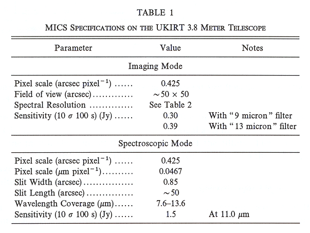
In the spectroscopic mode of the MICS, we can obtain the whole N‐band spectrum with a resolving power of 100 in one exposure. The pixel scales of both imaging and spectroscopy modes are set to achieve a diffraction‐limited spectral resolution. When it is attached to the UKIRT at the Mauna Kea observatory, the design goal of the spatial resolution is about 0 8. The specifications of the MICS are summarized in Table 1.
 |
2.2. Optics
The MICS optics were designed to achieve the diffraction limited spatial resolution both in imaging and spectroscopy modes. A final focal ratio of 10.5 was chosen. The optics for spectroscopy were designed to cover the whole N band (7.6–13.6 μm) in one exposure.
The optical components are illustrated in Figure 1, and the optical configurations are shown in Figure 2. The optics consist of three blocks: the pre‐optics, the spectroscopic optics, and the imaging optics.
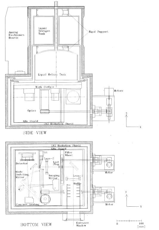
Fig. 1.— Structural configuration (the UKIRT version). The upper drawing is a cutaway view from the side, and the lower from the bottom. The dashed line in the lower drawing shows the optical axis.
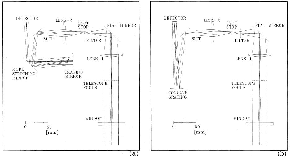
Fig. 2.— Optical design of the spectroscopy (a) and imaging (b) modes. All optics except for the entrance window are put in the cryostat and cooled with liquid helium.
The spectroscopic and the imaging optics employ reflecting mirrors. All mirrors are made of the same aluminum alloy as the baseplate, and thus the thermal contraction should not affect the image quality. The optical alignment was adjusted at room temperature.
The observing mode can be switched from imaging to spectroscopy (and vice versa) by extracting (inserting) a flat mirror and inserting (extracting) a slit.
2.2.1. Pre‐Optics
The pre‐optics package converts the incident beam from the telescope into a beam with the focal ratio of 10.5, the same as the final one. It consists of a germanium (Ge) entrance window, two Ge lenses, a filter wheel, and a Lyot stop. The incident focal ratios are F/36 for UKIRT, F/18 for the ISAS 1.3 m telescope (The Institute of Space and Astronautical Science, Sagamihara, Japan), and F/45 for the Mount Bigelow 61 inch telescope (Steward Observatory, Arizona). The configuration can be easily changed by exchanging one of the Ge lenses. At UKIRT, the ISAS telescope and the Mount Bigelow telescope, the pixel scales are 0.425, 1.24, and 1.04 arcsec pixel−1, respectively.
The telescope focus is located between the entrance window and the first lens (Lens‐1). The ray enters the Dewar through the window and passes through the first Ge lens, the filter wheel, the Lyot stop, and the second Ge lens (Lens‐2), and it makes an image on the slit position. The Lens‐1 also makes an image of the secondary mirror of the telescope on the Lyot stop to suppress unwanted thermal emission. The beam between Lens‐1 and Lens‐2 is nearly collimated with a diameter of 3.2 mm.
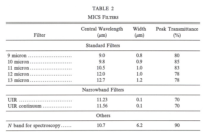
The filter wheel has seven one inch holes. One of them is for a wide N‐band filter for spectroscopy and another is blind for taking a dark image. The other five are used for imaging observations. The filters in use at present are listed in Table 2. Five of them ("9 micron," "10 micron," "11 micron," "12 micron," and "13 micron") are the N‐band standard "silicate" filters manufactured by Optical Coating Laboratory, Inc. All filters are tilted about 2° against the optical axis in order to avoid ghost images by surface reflection of the filters. The filter wheel is driven by a stepper motor mounted on the outside of the Dewar.
 |
2.2.2. Spectroscopic Optics
The dispersing element of the spectroscopic optics is a concave grating made of aluminum alloy. The surface is coated with gold. The focal ratio of the reflected light is the same as that of the incident light from the pre‐optics.
The concave grating allows us to make the optics small and compact, since collimator and camera optics are not necessary. The grating groove separation was varied to minimize astigmatism and distortion. A similar grating was used for the Mid Infrared Spectrometer (MIRS; Roellig et al. 1994) on the Infrared Telescope in Space (IRTS; Murakami et al. 1996). A detailed description about this type of grating can be found in Harada et al. (1980) and Onaka (1995).
The beam size on the grating is 14.3 mm in diameter and the groove spacing at the center is 10.67 mm−1. The resolving power of the grating is about 100, and the plate scale is 0.047 μm pixel−1 on the detector.
The slit is inserted at the position of the image made by the pre‐optics. The slit width is 150 μm, corresponding to 2 pixels on the detector, and the slit length is 9.6 mm. The slit is driven by an electromagnetic coil. Since the repeatability of the slit position is quite good (<15 μm, corresponding to 0.2 pixel) and there is no other movable component in the spectroscopic optics, the wavelength assignment to each pixel can be regarded as being fixed throughout observations. Therefore, we can minimize the number of wavelength calibrations, allowing efficient observations.
2.2.3. Imaging Optics
A toroidal mirror is used as an imaging element. Its surface figure is an ellipse whose two foci are located at the center of the detector and the center of the slit position. The plate scale of the reflected light is the same as that of the incident light. This mirror is made of aluminum alloy coated with gold. This is driven by a stepper motor via gears and shafts and they have free gaps. To reduce the gaps and fix the switching mirror position accurately, a pointing mechanism with a spring is employed. When the switching mirror is set into the imaging position, a spring‐loaded stop like a finger pushes the mirror back and removes the free gaps.
2.3. Cryogenics
All optical components except for the entrance window are mounted on the baseplate attached to the liquid helium tank and are cooled to 4 K. The temperature is cool enough to avoid excess noise by thermal radiation from the optical components. They are enclosed by an inner radiation shield at liquid helium temperature, which is also enclosed by an outer radiation shield at liquid nitrogen temperature to minimize a light leak and extend the holding time of liquid helium.
The detector is mounted on the cold baseplate. However, the temperature changes with its heat generation, which depends on the integration time. To keep the detector temperature stable, we apply a small amount of extra heat to the detector module by a resistive heater. The heater is controlled by a temperature controller manufactured by Lakeshore, and the lowest stable temperature is 6 K.
The holding time of liquid helium is 20 hours or more, and that of liquid nitrogen is 24 hours without running the detector. The heat load from the running detector and the heater makes the holding time of liquid helium to about 16 hours. This is still long enough for observations over one night.
2.4. Electronics
2.4.1. Detector and Driver Electronics
The MICS employs a Si:As Block Impurity Band (BIB) array for moderate flux manufactured by Rockwell International. The BIB detector is one of the best detectors in the mid‐infrared (cf. Bharat 1994; Noel 1992). The array format is 128 × 128 with a pixel size of 75 μm. This was the largest format detector for the mid‐infrared when this project started. The characteristics of the detector are summarized in Table 3.
 |
The signals can be read without resetting the signal integration (nondestructive readout), which allows us to apply a multiple sampling method. We usually use subtractive double sampling in which a signal for each pixel is sampled twice, before and immediately after the reset, and the difference between the sampled signals is regarded as the count for the pixel. This method is effective for canceling out fluctuation of reset bias and reducing readout noise.
To read out the detector signals, four clocks and 10 DC biases are required. A block diagram of the electronics system and a schematic drawing of the driver electronics are shown in Figures 3 and 4, respectively. The detector clocks are generated by the Clock Pattern Generator (CPG) board as TTL signals in the VME rack. The CPG board also generates timing clocks for the Analog‐to‐Digital (A/D) converters, the co‐adder circuits, and the secondary chopper controller. The voltages of the detector clocks are shifted to the suitable level of the detector (+3/+7 V) on the detector‐driver board in the analog electronics box which is attached on the Dewar. All DC biases are generated on the same detector‐driver board.
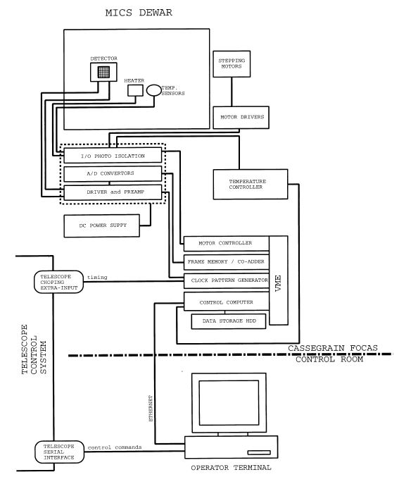
Fig. 3.— Block diagram of the MICS control system. All components above the dot‐dashed line are mounted at the Cassegrain focus of the telescope, and the others are located in the control room. The dashed box shows the analog electronics box attached on the Dewar.
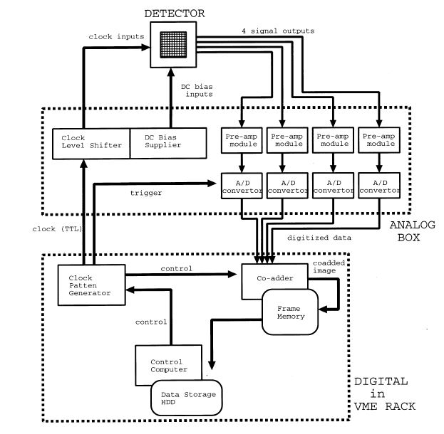
Fig. 4.— Schematic drawing of the control and readout system of MICS
2.4.2. Data Acquisition System
In mid‐infrared observations, a large number of background photons usually falls into each pixel of the detector. The background flux of the imaging with a bandpass filter (Δλ∼1 μm) in the N band is about 2 × 10⁸ e s−1 pixel−1. The full well of the MICS detector is 107 e− pixel−1 and the saturation level of the A/D converters is set as about 7 × 10⁶ e− pixel−1. Therefore, we adopt 40 Hz as the typical frame rate.
The data acquisition system is shown in Figure 4. The detector has four outputs, and the signal from each output is led into each preamplifier. The amplified signals are digitized by four 1 MHz sampling 16‐bit A/D converters.
The preamplifiers and the A/D converters are installed in the analog electronics box with the bias suppliers and the clock level shifters.
The digitized data are led into the digital board, co‐added in the hardware co‐adder circuits, and stored as 32 bit pixel−1 data in the frame memory. The frame memory can be read directly by the control computer. When an integration is completed, stored data in the frame memory are transferred into a storage hard disk of a control computer. The production rate of the data is 66 kbyte per frame and 2.5 Mbyte s−1.
The data are stored in the FITS format, and observational parameters (frame rate, observing mode, detector temperature and so on) are written in the file header.
2.4.3. Control Software
The whole system is controlled by the computer, which is a Sun‐workstation compatible machine, Force Computer CPU‐5V, and is mounted on a VME rack on the telescope. Observers can control this computer via ethernet from the console of the second computer in the control room.
The MICS control software consists of short programs written in the C language. These programs run in the control computer, and each program makes a simple task as a command line. This method has a great advantage for developers to make and revise the programs. At actual observations, however, command‐line operation may not be convenient. Therefore, a managing software running in the second computer is used for convenient operations. The observers can generate a series of basic commands and send them to the control computer only by inputing the observational parameters, such as the integration time and the chopping frequency, into the management software via a graphical user interface.
3. PERFORMANCE
3.1. System Efficiency
System efficiency including the optical throughput and the detector efficiency was measured to be 13% [electron/photon] in the imaging mode with the "10 micron" filter (Δλ∼1 μm) and 9% in the spectroscopy mode.
The quantum efficiency of the detector is about 30%, and thus, the throughput of the optics, including the entrance window, two Ge lenses, mirrors, and filters is estimated as approximately 45%. This value agrees with the throughput estimated from the measurements of each optical component at room temperature. The ratio of the spectroscopic efficiency to the imaging efficiency is 70%, in agreement with the efficiency of the grating itself.
3.2. Response Linearity and Readout Noise
The linearity of the detector response was obtained from the relation between the integration time and the output count. The result is shown in Figure 5 and demonstrates a good linearity. The deviation from the fitted line is 0.3% or less in the output range of less than 6 × 10⁶ e−.
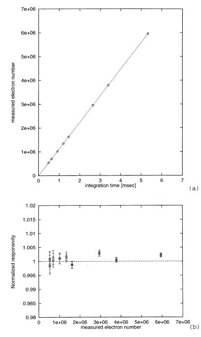
Fig. 5.— Linearity of the MICS detector. (a) Relation between the integration time (vertical axis) and the output count (horizontal axis) for a constant flux level. The dashed line shows the fitting result. (b) Normalized responsivity of each output count. It is clearly indicated that the deviation from the linearity is less than 0.3%.
The readout noise is 770 electrons per readout in the subtractive double sampling mode. This noise value is about a quarter of the shot noise caused from the full well. Thus, the readout system achieves the shot noise limited performance.
3.3. Dark Current
The dark current was measured as a difference between the output count of short (∼25 ms) and long (∼500 ms) exposure under complete dark condition of the array. The measured dark current was 4 × 10⁵ e− s−1 pixel−1 at the detector temperature of 6 K.
For comparison, the background radiation generates about 2 × 10⁷ e− s−1 pixel−1 in spectroscopic observations and 2 × 10⁸ e− s−1 pixel−1 in imaging observations. The dark current generates less than 2% extra noise in excess of the background noise.
The dark current strongly depends on the detector temperature. It becomes larger by about 10 times at 8 K than at 6 K. We use a temperature controller and keep the detector clocks running during observations. With this method the detector temperature is kept stable at 6 K within 0.01 K. Any extra noise attributable to the temperature fluctuation has not been detected.
3.4. Radiation Shielding
Twofold radiation shields kept at the liquid helium and the liquid nitrogen temperatures, as described in § 2.3. The thermal radiation from emitters at liquid nitrogen temperature might be detected as excess "dark current," because the spectral response of the detector extends to about 26 μm.
In order to evaluate stray radiation, we measured the dark current with a blind filter on and the cooled cover in front of the detector off. The measured value is twice the pure dark current, indicating that the incomplete shielding causes photo current as high as the pure dark current, about 4 × 10⁵ e− s−1 pixel−1. This is still small compared to the background photon and we conclude that the stray radiation from liquid nitrogen temperature does not affect the performance. We have also confirmed that the stray radiation pattern was quite stable and did not produce extra noise in the observations.
3.5. Performance on UKIRT
In order to evaluate the performance of the MICS when mounted on a telescope, we carried out test observations with the Mount Bigelow 61 inch telescope and UKIRT during 1996 and 1997. In the rest of this paper, we will discuss the data taken at UKIRT during 1997 September 17–19. We note that the humidity was less than 7% and the sky condition was very good at the observing time.
3.5.1. Point Spread Function
Figures 6a, 6b, and 6c show stellar images taken by the MICS to obtain the point spread function (PSF). They are the images of β Peg obtained in the imaging mode with the 9 micron, 10 micron, and 13 micron filters, respectively. Each image is the sum of 39 frames and the integration time of each frame is 25 ms. These data were taken by using the tip‐tilt secondary system of UKIRT.
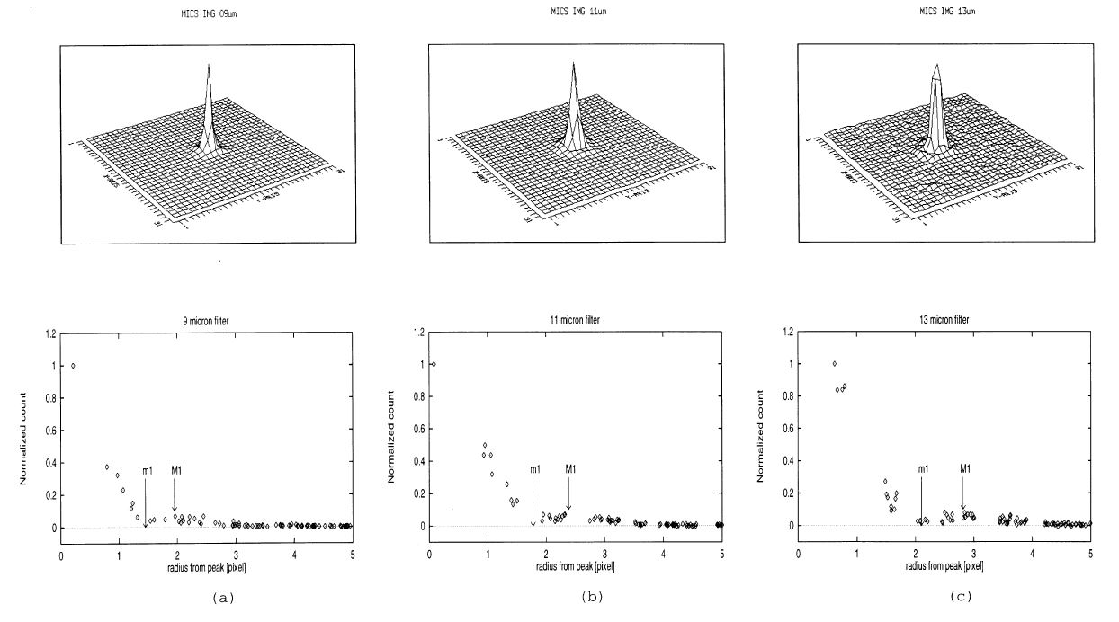
Fig. 6.— Surface brightness maps (upper panels) and the radial energy distributions (lower panels) of β Peg obtained in the imaging mode. The integration time of each image was 975 ms. The spatial scale is in units of pixel, and 1 pixel corresponds to 0425. The labels "m1" and "M1" in the lower panels indicate the position of the first dark and the first bright rings of the Airy function, respectively. (a) With the "9 micron" filter; (b) "11 micron" filter; (c) "13 micron" filter.
The first Airy rings are visible in all images, which demonstrates that the diffraction‐limited performance has been achieved. The full widths at half‐maximum (FWHM) are estimated to be 1.7, 2.0, and 2.4 pixels (1 pixel = 0425) for 9, 10, and 13 micron images, respectively.
The PSFs of the spectroscopy mode at three wavelengths are shown in Figure 7. These are obtained by slicing a observed spectrum of β Peg along the slit direction. The estimated FWHMs are 2.0, 1.8, and 1.9 pixels at 9, 11, and 13 μm, respectively. These values correspond to the spatial resolution of about 08.
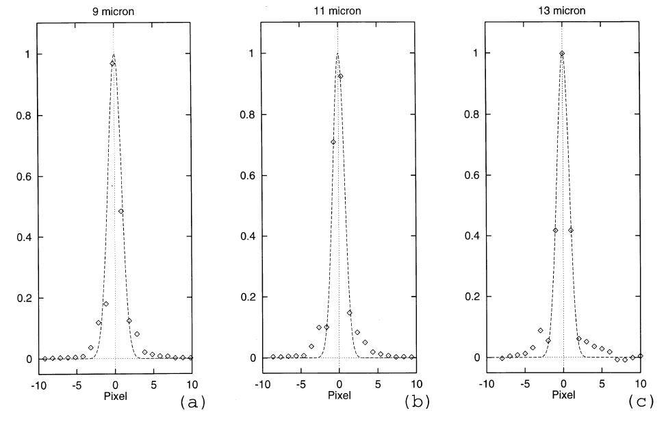
Fig. 7.— Point spread functions (PSFs) in the spectroscopy mode. The object was β Peg and the integration time was 2.51 s. Each panel shows the count along the slit direction at each wavelength. The counts are co‐added for 2 pixels along the dispersing direction (Δλ∼0.1 μm) and normalized at the peak. The broken lines show the results of Gaussian fit for the central 5 pixels. (a) PSF at 9.0 μm; (b) PSF at 11.0 μm; (c) PSF at 13.0 μm.
We conclude that the MICS has achieved the diffraction‐limited spatial resolution of the telescope diameter in imaging as well as in spectroscopy.
3.5.2. Spectral Resolution
The performance in the spectral resolution was estimated from the line profiles of astronomical objects. Figure 8a shows a spectrum of a massive star‐forming region, W51 IRS2 East, obtained by the MICS (Okamoto et al. 1999). Three fine‐structure lines, [Ar iii] 8.99 μm, [S iv] 10.51 μm, and [Ne ii] 12.81 μm can be seen in the spectrum. Figures 8b–8d display the line profiles. The FWHMs of these lines are less than 2 pixels (∼0.093 μm). Since the intrinsic profiles should be much narrower than 0.093 μm, the instrumental spectral resolution can be derived as 90 at 9 μm and 130 at 13 μm. These values agree well with the designed values.
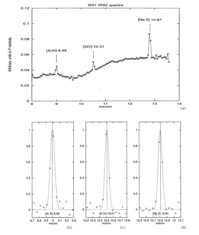
Fig. 8.— Spectrum of a massive star‐forming region, W51 IRS2 East. The on‐source integration time was 9.74 s. The slit width was 085 and the spectrum was co‐added for 62 along the slit. (a) The spectrum between 8.0 and 13.6 μm is shown. Three fine‐structure lines, [Ar iii] at 8.99 μm [S iv] at 10.51 μm and [Ne ii] at 12.81 μm can be clearly seen. (b) Detailed profile of the [Ar iii] line. Because the line width is intrinsically much narrower, it directly indicates the spectral resolution of the MICS. (c) Same as (b), but of [S iv]; (d) same as (c), but of [Ne ii].
3.5.3. Sensitivity
The sensitivity of the MICS when mounted on UKIRT was derived from the observed images and spectrum of β Peg. We adopted the absolute flux of β Peg provided by M. Cohen (private communication).
In the imaging mode, we evaluated the absolute flux scale, based on the measured counts and the stellar absolute flux. The noise was derived from the fluctuation in the count of blank sky region and converted into flux. The noise equivalent flux (NEF) estimated from the fluctuation of the blank sky in imaging mode with the "9 micron" filter is 170 mJy pixel−1 for 1 s integration, or 0.40 Jy arcsec−2, and thus the NEF for a point source is estimated as 0.30 Jy. This agrees well with the signal‐to‐noise ratio estimated from the fluctuation of the stellar count of each image.
The sensitivity in the spectroscopy mode was derived in the same way as that in the imaging mode. The slit throughput depends on the wavelength, because the slit width (150 μm) is very close to the diffraction limited size. The throughput was estimated as the ratio of the stellar spectrum obtained with the slit to that obtained without the slit, being 61 ± 3% at 9 μm, 58 ± 3% at 11 μm and 56 ± 6% at 13 μm. They can be fitted as (76 - 1.54 × λ)%, where λ is the wavelength in microns.
Using this relation, we estimate that the NEF is 0.49 Jy pixel−1 at 11.0 μm with the bandwidth of 0.1 μm, where the telluric absorptions are minimum in the N band. The sensitivity in the spectroscopy mode for a diffuse source is typically 1.5 Jy arcsec−2, and that for a point source is 1.4 Jy. The estimated sensitivities are summarized in Table 1.
4. SKY NOISE AND OBSERVING TECHNIQUES IN THE N BAND
Because of the enormous background emission in the N band, it is very important to subtract the background flux accurately. The background emission comes from the sky and the telescope. The emission from the sky has a large time variation both in the amount and the spatial pattern. Inaccurate cancellation of the background emission results in extra noise called "sky noise."
In this section, we will describe the sky noise based on observations by the MICS and discuss effective observing methods in the N band. All the data used in this section were obtained in the test observations on UKIRT in 1997 September.
4.1. Sky Noise
The sky noise was evaluated from the blank sky spectra obtained at an interval of 50 ms. We calculated the Fourier power spectrum of the fluctuation at seven wavelengths. The results are shown in Figures 9. Each panel shows the Fourier power of the noise at each wavelength. A broken line in each panel shows the shot noise power, which is estimated from the absolute count.
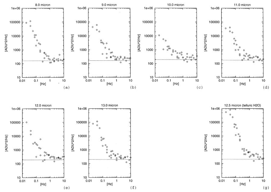
Fig. 9.— Power spectra of the noise evaluated from the fluctuations of the blank sky spectra obtained in the spectroscopy mode. The count was co‐added for 50 pixels along the slit direction, which corresponds to 213, and for 2 pixels along the dispersing direction, which corresponds to Δλ∼0.1 μm. The horizontal axis indicates the frequency (Hz) and the vertical axis indicates the Fourier power of the noise (arbitrary units). (a) Noise power at 8.0 μm; (b) 9.0 μm; (c) 10.0 μm; (d) 11.0 μm; (e) 12.0 μm; (f) 13.0 μm; (g) 12.5 μm (including the strong atmospheric water emission).
Figure 9 demonstrates that the noise power is almost constant above 0.5 Hz and becomes larger below 0.5 Hz. The constant level above 0.5 Hz is roughly equal to the power of the shot noise, and the excess below 0.5 Hz was not seen when the system is blanked off. Therefore, the excess can be attributed to the sky noise.
Figure 9 also indicates that dependence of the noise on the frequency is different at different wavelengths. The noise power at the center of the N band (10 or 11 μm) is lower than that of the edges of the N band (8 and 13 μm). At the wavelength range where an atmospheric water vapor line (12.5 μm) is present, the noise power is much higher than any other wavelengths (see Fig. 9g).
The dependence of the sky noise on the wavelength is clearly demonstrated as shown in Figure 10. The noise power is much higher at particular wavelengths, 11.8 and 12.5 μm. These wavelengths correspond to the positions of atmospheric water vapor lines (Figs. 10d and 10e). In contrast, there is no strong excess at the wavelengths of telluric ozone bands (9.5–10 μm). These facts indicate that the ozone emission is more stable than the water vapor emission.
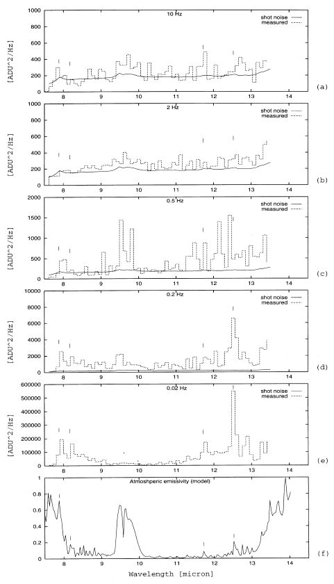
Fig. 10.— Noise power vs. wavelength. (a) Noise power at 10 Hz. The solid line shows the shot noise level expected from the count. The vertical short lines indicate the position of the atmospheric water vapor emissions, 7.882, 8.170, 11.722, and 12.522 μm. (b) at 2.0 Hz, (c) at 0.5 Hz, (d) at 0.2 Hz, (e) at 0.02 Hz. The shot noise level is drawn but cannot be seen. (f) The atmospheric emissivity calculated by the ATRAN software (Load 1992).
The water vapor emissions are thought to come mainly from invisible aerosols/cirrus clouds in the troposphere (Bensammar 1978), while the ozone emissions come from the higher (∼25 km) layer of the atmosphere, stratosphere. The stratosphere is more stable than the troposphere, which may result in the observed difference in spectral dependence of the noise power.
The frequency at which the sky noise is roughly equal to the shot noise is 0.5 Hz and constant in the N band. Kaeufl et al. (1991) measured the fluctuation of the background radiation and concluded that the sky noise in the N band was dominant in the frequency range below 8 Hz. Their measurements were carried out at the ESO‐site of La Silla (2400 m altitude) by using the photometric data taken with a wide‐band filter. The present results are derived from the spectroscopic data obtained at the Mauna Kea Observatory (4200 m altitude). The narrower bandwidth may be attributed to the weaker fluctuation of the background radiation, or, the higher altitude of the observing site may lead to the different result. Further observations are needed to investigate the dependence of the sky condition.
4.2. Effective Observing Methods in the N Band
4.2.1. Self‐Sky Subtraction
When a two‐dimensional array is used, many pixels usually observe blank sky. Therefore, the background could be subtracted by the blank sky around the targets in principle. This is so‐called "self‐sky subtraction," and seems effective because the sky is simultaneously measured when the targets are observed.
However, in practice, the background cannot be subtracted by this method accurately in the N band, because of inaccuracy of the flat‐fielding. The background radiation of imaging observations generates 2 × 10⁸ e− s−1 pixel−1, which corresponds to 100 Jy pixel−1 when the MICS is attached on UKIRT. The NEF of imaging observation is 170 mJy pixel−1 (see § 3.5.3). Therefore, the accuracy of the flat‐fielding is required to be better than 0.2%.
The flat‐fielding is made using the blank sky images, which are obtained at different airmass positions. The flat‐field error becomes up to 3% in maximum. This is less accurate than required. Therefore, the self‐sky subtraction is not useful and the measurement of background by the same pixels as that of targets is needed for sensitive observations in the N band. The secondary mirror chopping is one of the most effective methods for it.
4.2.2. "Chop and Nod" Technique
To cancel the effect of sky variation, we subtract the sky image obtained immediately before and/or after the target image by using the secondary mirror chopping. The frequency of the chopping must be faster than frequency of the time variation of the sky background pattern. The measurement of the blank sky discussed in the previous section (Fig. 9) suggests that the sky noise is dominant below 0.5 Hz for all wavelengths. Thus, the chopping frequency should be faster than 0.5 Hz.
To demonstrate the effect of the chopping, we took blank sky spectra with various chopping frequencies and derived the noise at each wavelength. The chopping throw was 108. The results are shown in Figure 11. The measured noise almost equals to the shot noise in the range of the frequency above 0.5 Hz, while it is about 3 times larger than the shot noise at the frequency of 0.2 Hz. These results give good agreement with the measurements of the sky noise discussed in the previous section.
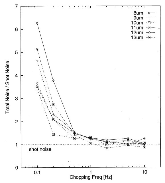
Fig. 11.— Relation between the chopping frequency and the noise. The noise is measured from the blank sky spectra and normalized by the shot noise expected from the count at each wavelength (for 8 μm, diamonds and solid line; 9 μm, crosses and dashed line; 10 μm, squares and short‐dashed line; 11 μm, crosses and dotted line; 12 μm, triangles and dot‐dashed line; 13 μm, stars and dot‐short‐dashed line). Strong excess noise appears below 0.5 Hz.
Because the chopping is performed by wobbling the secondary mirror, different patterns of the background emission from the telescope could appear. This yields a residual pattern after the chopping subtraction is made. The absolute amount and pattern of the residuals depend on the telescope and the chopping throw. In case of UKIRT, the flux of the residuals is about 1 Jy pixel−1, which is almost 6 times larger than the shot noise generated by 1 s integration in the imaging mode. To cancel out these residuals, the nodding of the primary mirror must be carried out. Consequently, this observing process we adopted is so‐called the "chop and nod" technique.
The effectiveness of the nodding depends on its time interval. No residual pattern was detected when an interval of 30 s and a throw of 208 was used. At this time interval, the nodding removes the residuals almost completely (<10 mJy pixel−1). The nodding with intervals of 1, 3, and 5 minutes left the residuals of about 20, 50, and 70 mJy pixel−1, respectively. The interval of the nodding should be shorter than 30 s. This value may vary with telescope, observing condition, and chopping throw.
While the background‐noise limited sensitivity is almost achieved with the chop and nod technique, the observing efficiency is another concern. If the object is compact enough, it is possible to put all images obtained in four beams of the chop and nod on the detector and to avoid the loss of net integration time. This produces four images of the objects, two positive and two negative ones. One can observe objects without the loss in efficiency if they are smaller than 25'' × 25'' in imaging mode and 12'' in spectroscopy mode. If the object is larger, the chopping throw and/or the nodding throw should be larger than the object size. In this case, some of the four images will be put off the detector, and the efficiency will be decreased by a quarter in the worst case.
5. SUMMARY
We have developed the Mid‐Infrared Camera and Spectrometer (MICS) for ground‐based observations. This is an instrument optimized for observations in the N‐band (7.6–13.6 μm) atmospheric window, and it has two observing modes: imaging and long‐slit spectroscopy. In the spectroscopy mode, the MICS covers the whole N band with a resolving power of 100 in one exposure. The spatial resolution of the diffraction limited performance has been achieved both for imaging and spectroscopy.
We evaluated the sky noise in the N band from the MICS observations. The sky noise was dominant below 0.5 Hz, implying that the chopping frequency should be faster than 0.5 Hz. The sky noise has excess at the positions of atmospheric water vapor lines than those without water vapor lines, while it does not show excess at the positions of the atmospheric ozone feature.
We confirmed that the background‐noise limited sensitivity can be achieved when chopping with 0.5 Hz or faster and nodding with an interval of 30 s or shorter. The noise equivalent flux of 1 s on‐source integration in imaging and spectroscopic observations is 0.3 and 1.2 Jy, respectively.
We wish to acknowledge Prof. T. Geballe and Dr. A. Chrysostomou at Joint Astronomy Centre for their support in the UKIRT observing run. We thank the UKIRT staff, particularly S. Arakaki for his help in preparing the run. We also acknowledge Prof. T. Nishimura for continuous support, the staffs of Advanced Technology Center of National Astronomical Observatory of Japan in the development of the MICS, Dr. T. L. Roellig for latest information on the mid‐infrared array detectors, Dr. M. Cohen for providing the calibrated spectrum of β Peg, and Dr. M. Ruitz and Dr. A. Harrison for useful comments to this paper.
This work was supported in part by Grants‐in‐Aid from the Ministry of Education, Science, Sports and Culture in Japan, special grant from University of Tokyo, and the National Astronomical Observatory of Japan. T. M. was supported by the JSPS fellowships for Japanese Junior Scientists.