
ABSTRACT
The Antarctic Fiber Optic Spectrometer (AFOS) is one of a suite of instruments of the Automated Astrophysical Site Testing Observatory (AASTO) installed at the South Pole in 1996 December. In 1998, the AFOS will be attached to an altitude‐azimuth mount and commence regular astronomical observations. In the years 1998–2000, the AASTO will be moved to other remote locations, high on the Antarctic plateau, in order to complete the site testing campaign. The AFOS experiment consists of a 30 cm Newtonian telescope injecting light into a 45 m length of optical fibers that feed a UV‐visible (200–840 nm) grating spectrograph inside the warm shelter. In this paper we describe the instrument and the first results. The main requirement of the design was reliable operation in an extremely cold environment, without maintenance, for 12 months. This has been achieved despite the very low power (approximately 7 W) available to run the instrument.
Export citation and abstract BibTeX RIS
1. INTRODUCTION
The Antarctic plateau offers very favorable conditions for certain kinds of astronomical research (Burton et al. 1994). These conditions are now being quantified by the Automated Astrophysical Site Testing Observatory (AASTO) experiment. The AASTO itself is based on technology developed by Lockheed for the US Automated Geophysical Observatory (AGO) program (Doolittle 1986) but incorporates a number of significant improvements.
The AASTO is basically a propane‐powered well‐insulated shelter that keeps itself warm and generates 50 W of continuous electrical power, shared by several instruments, for a full 12 months.
The AASTO will eventually be equipped with a full suite of astronomical instruments (Storey, Ashley, & Burton 1996). Three of these are currently in operation: the AFOS (this paper) and near‐ and mid‐infrared sky monitors (NISM and MISM). The AFOS consists of a 30 cm telescope that injects light into a 45 m length of optical fibers. The fibers lead back to the AASTO shelter, in which is located an imaging grating spectrometer with a CCD detector.
It was decided to locate the telescope on a tower, about 35 m upwind from the AASTO, in order to minimize snow drifting and locally generated air turbulence problems. A photograph of the installation at the South Pole is shown in Figure 1. These requirements are also partly imposed by the second instrument to be mounted on the tower (in 1997–1998): a Differential Image‐Motion Monitor being built by Mount Stromlo and Siding Spring Observatories (Dopita, Wood, & Hovey 1996).
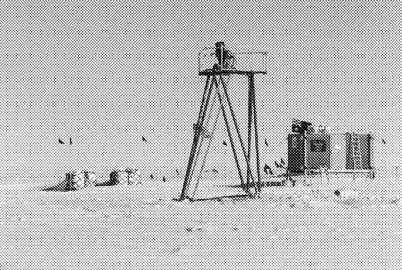
Fig. 1.— Installation at the South Pole, 1997 January
As with all the AASTO instruments, the AFOS is constrained to consume an average power of less than 7 W and to operate unattended for 1 yr in conditions of extreme cold (down to −90°C), wind (up to 20 m s−1), and accumulation of snow and ice. A considerable number of interesting technological challenges are presented by this severe environment.
2. SCIENTIFIC GOALS
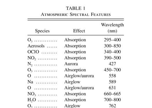
The AFOS is a UV‐visible site testing instrument optimized to obtain data on the quality of the sky for astronomical observations. A similar instrument (Roscoe et al. 1994) dedicated to stratospheric measurements is in operation at Halley, the British Antarctic base. Our goals are to observe the UV cutoff wavelength of the atmosphere, the depth of various molecular absorption bands affecting the atmosphere's transmission, and the strength of airglow and auroral emission lines. Table 1 summarizes the atmospheric constituents that contribute to these phenomena.
 |
All radiation at wavelengths below 295 nm is absorbed by atmospheric gases, mainly the Hartley band of ozone. In the near‐ultraviolet (295–400 nm), the radiation is partially absorbed by the Huggins band of ozone (mainly in the region λ<320 nm); part is backscattered into space, but a significant amount still reaches the Earth. The lower column density of ozone over Antarctica should result in a substantial decrease in the UV cutoff wavelength.
Atmospheric transmission measurements are usually made by observing the same star at different elevations: any differences can be attributed to the additional air mass through which the light has passed. However, this cannot be achieved at the geographic South Pole where the stars have the same elevation all night long. We will instead observe different stars of the same spectral class.
3. TELESCOPE
3.1. Optical Characteristics
3.1.1. Configuration
We chose a Newtonian configuration as a good compromise between possible telescopes types. A prime focus system would have been too long, and a Cassegrain telescope unnecessarily complex and expensive. The telescope has been built with the supporting mount specifications in mind and, in particular, a maximum allowed swing radius of 600 mm and weight of 80 kg.
3.1.2. Optics
The primary parabolic mirror has a diameter of 318 mm and a focal ratio of 3.35. It is made from Astrositall, a glass with a low thermal expansion coefficient1 of α = 0.15 × 10⁻⁶ K−1. It was given a UV‐enhanced aluminum coating of Al‐MgF2 (yielding 85% reflectivity from 300 to 850 nm). The secondary is an elliptical flat mirror at 45° with a major axis of 108 mm and produces 6% obscuration. It is a commercial Pyrex product (α = 3.2 × 10⁻⁶ K−1) with a UV‐enhanced coating. The telescope tube is closed by a front window (which is also the aperture stop) with a diameter of 290 mm. It is 10 mm thick and is made from fused silica with a transmission of 92% over the range 300–850 nm; an antireflection coating was not used.
3.1.3. Adjustments
The telescope is designed neither to require nor to offer any degree of adjustment, thus avoiding any long‐term instability. Careful manufacturing and the use of shims under the primary mirror were used to align all the optics. The primary mirror is held in a standard cell with three fixed points of contact, three lateral supports (one is removable), and three retaining pads on the mirror surface (spring plungers). After several disappointing tests of glues (which, although rated for low‐temperature applications, proved inadequate), the secondary mirror was simply glued with RTV silicone directly onto the spider subassembly. It is worth noting that RTV silicone becomes quite hard at temperatures below −30°C but does not become brittle and so is a suitable glue for many low‐temperature applications. The entrance window was compressed onto an O‐ring by an external holder.
3.2. Mechanical Characteristics
3.2.1. Material Used
A critical requirement of the telescope was its ability to remain focused and collimated over a temperature ranging from + 20°C to −90°C. An athermalized design was therefore essential. We chose materials with very low thermal expansion coefficients. All the mechanical parts (including the fiber optics injection module) were made from Invar 36 (α = 0.9 × 10⁻⁶ K−1). A further advantage of this method of athermalization is that the differential thermal expansion among the materials used (Invar, Astrositall, Pyrex) is negligible and does not create any significant mechanical stress on the optics.
We also investigated the alternative approach of using an all‐aluminum design for the mechanical and optical components. This would have resulted in a light and easy‐to‐machine structure, but the preparation of aluminum mirrors for UV applications is difficult and expensive. An all‐Pyrex design was also considered, but a large Pyrex telescope tube would be too heavy for the mount.
3.2.2. Tube Fabrication
The tube (Fig. 2) was made from a rolled Invar sheet (1.6 mm thick), which was TIG welded. A closed square box section holds it in the middle and presents an interface to bolt the telescope onto the mount. External reinforcing webs were welded longitudinally to the tube to increase stiffness. Two flanges were bolted at each extremity of the tube, the bottom one for locating the primary mirror support plate, and the upper one for mounting the window holder. Finally, the structure was stress relieved prior to final machining and optical alignment by heat treatment for 1 hr at 400°C followed by air cooling.
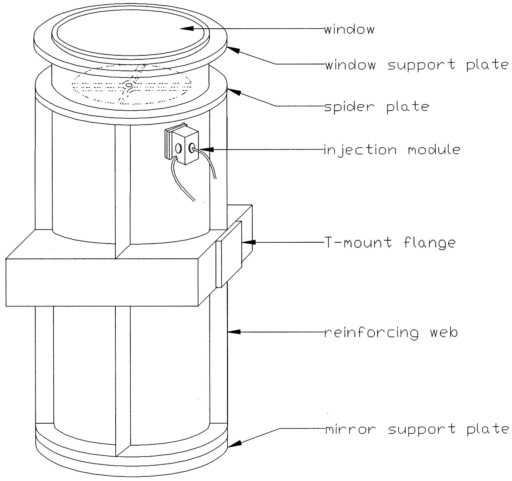
Fig. 2.— General view of the telescope structure
3.2.3. Spider
The small field of view (100 μm ≈ 20 '') of the optical fibers at the focus of the telescope makes the design of the spider critical. This structure must be rigid enough to avoid bending or twisting with gravity. The spider (four arms, each 6 mm wide) and secondary mirror holder were cut as one single piece from an Invar plate (7 mm thick). A water‐jet cutter was used in order to avoid introducing stress. NASTRAN modeling of the telescope indicated that the maximum deflection of the tube, in going from the zenith to the horizon, creates a displacement of the optical axis of only 15 μm in the focal plane.
3.2.4. Seals
A major problem with all instruments operated in the cold is frosting of the optical surfaces. This is a constant challenge, and it requires a lot of care to implement an effective solution. Good practices include careful sealing using O‐rings on all removable parts, then flushing the inside volume with High Purity Grade dry nitrogen (which nevertheless still has 10−4% water content) before sealing (with a small positive pressure in the volume), and using an internal desiccant to remove any remaining water vapor (at least to a final partial pressure of water lower than the vapor pressure of ice at −90°C). If this process is not perfect, the remaining water will freeze on the coldest surface, which, in a telescope, is usually the entrance window.
We used fluorosilicone O‐rings (which stay flexible at low temperatures) and a canister filled with about 50 g of finely ground calcium hydride (CaH2), attached to the AFOS telescope tube with a standard vacuum KF flange. CaH2 was chosen because the equilibrium water vapor pressure above it is only 10−5 mm Hg, well below the 7 × 10⁻⁵ mm Hg vapor pressure of ice at −90°C (Schriver 1969, p. 194). The CaH2 powder was placed behind a Gortex membrane to allow water vapor to pass and to keep the powder in one place. Reaction of CaH2 with the residual water vapor generates hydrogen gas. However, the quantities involved in this application are very small and should not create problems.
"Diamond dust," composed of micron‐sized cylindrical crystals of ice, is a common phenomenon in Antarctica. It can penetrate any small gaps and rapidly fill large volumes. To prevent this problem, and more generally to avoid accumulation of snow, all the external surfaces of the telescope must be as flat and smooth as possible and properly sealed.
Finally, we used a Brownell bidirectional pressure relief valve, set to open at a differential of 0.15 psi (at −80°C), in order to prevent dangerous pressures from building up. This allows some "breathing" of the telescope air space, which effectively increases the volume of air that the CaH2 desiccant has to process during the year. We calculated the importance of this effect by using historical atmospheric pressure/temperature data from the 1995 South Pole records. As Figure 3 shows, this additional volume of air is small enough that the desiccant should easily be able to cope.
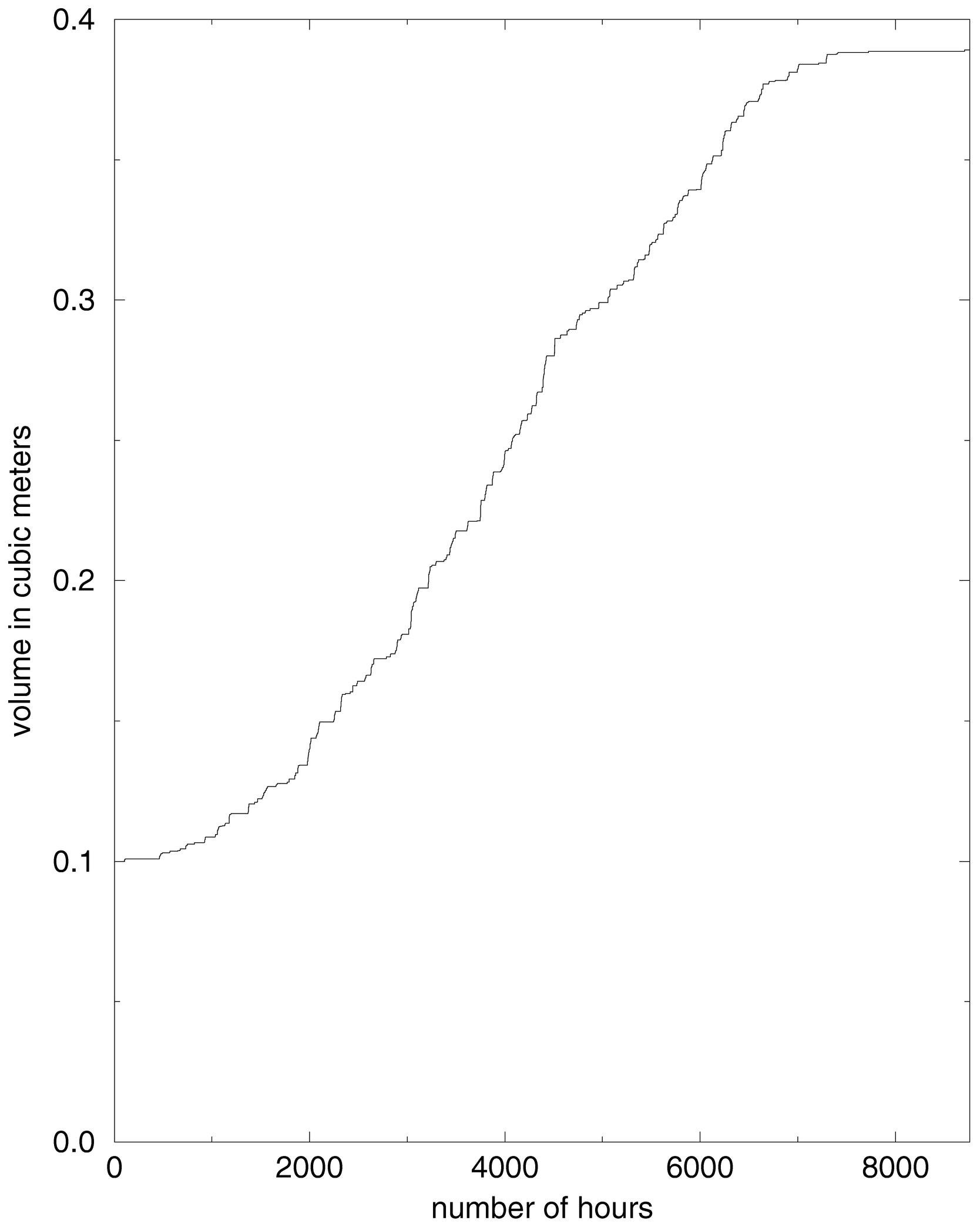
Fig. 3.— Cumulative volume of air that the desiccant within the AFOS telescope has to process as a function of time during the year, based on South Pole meteorological data for 1995. The enclosed volume of the AFOS is assumed to be 0.1 m3.
3.2.5. Deicing System
We have designed a system that allows the detection of ice formation on the entrance window and removes it if necessary. The ice sensor is formed by a ring of four LEDs in series, attached to the internal walls of the tube and illuminating the window from an oblique angle. Any formation of ice will create backscattering of the light into the optical system and will produce increased signal onto the detector. By comparing with a stored reference signal from a clear window, we can determine if the deicing system needs to be activated or if astronomical observations can continue.
After considering many possibilities, it appeared that the best approach to deice the entrance window was a heated aluminum plate placed in close proximity to the glass. Usually, a temperature differential of 5°C–10°C above ambient is sufficient to sublimate ice.
The heating cover is attached to the mount platform on a pivot axis and is balanced by a counterweight. When the telescope is parked and pointing toward the nadir, the front surface of the window is brought within 1 mm of the heater. The heater consists of 12 resistors, capable of dissipating a total of 20 W, bolted to a 6 mm thick aluminum plate insulated on the side away from the window.
A platinum temperature sensor is glued with RTV silicone to the center of the window on the inside surface. The window itself is mounted on a thin‐walled stainless steel structure welded to the top flange of the Invar tube. This was done in order to create a large thermal impedance and to minimize transfer of heat from the window to the Invar structure.
The window itself has a step machined around the edge and is compressed onto an O‐ring by a retaining ring. The resulting external surface is flat, and a ring of felt has been inserted between the glass and the holder to break the thermal path and to seal against ice crystals.
4. FIBER OPTIC LINK
4.1. Choice of the Optical Fibers
4.1.1. Fiber Type
A special UV‐enhanced fiber (high OH content) is necessary to achieve a reasonable transmission in the UV. These fibers have a deep OH absorption band at 730 nm. We would degrade the performance of our instrument in the red if we used only this fiber. In particular, we would have had to increase the integration time (as we need a very high signal‐to‐noise ratio) for the measurements of atmospheric H2O between 700 and 800 nm.
A second problem arises from the necessity to filter out second‐order light at wavelengths below 400 nm when observing between 600 and 800 nm. With a single fiber we would be unable to observe simultaneously in the blue and red regions of the spectrum.
Hence, we decided to use two types of fibers (see Table 2): a "blue" one (FV series from Polymicro Technologies 1994) and a "red" one (FI series from Polymicro Technologies 1994, ultra–low OH, without absorption in the red but with poor UV transmission). A dichroic beamsplitter (ideally with R = 100% from 300–550 nm and T = 100% from 550–850 nm) directs the light to the respective fibers. The separation at 550 nm is chosen because this is the wavelength at which both the red and blue fibers reach the same transmission (and there are no special observational requirements at this wavelength). This concept allows us to optimize the transmission from 300 to 850 nm and to make simultaneous observations over the entire spectrum, which gives an effective gain in observing efficiency.
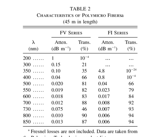 |
A 100 μm fiber core corresponds to a 19 6 of field of view (FOV) in the sky and 2.4 nm FWHM spectral resolution on the CCD. We chose it because, among the available fibers, that was our best compromise between decreasing core diameter resulting in difficulties centering the star image at the input of the fiber and putting more severe constraints on the 20
'' pointing accuracy of the mount, and increasing core diameter and losing spectral resolution (as the fibers themselves act as the entrance slit to the spectrometer).
6 of field of view (FOV) in the sky and 2.4 nm FWHM spectral resolution on the CCD. We chose it because, among the available fibers, that was our best compromise between decreasing core diameter resulting in difficulties centering the star image at the input of the fiber and putting more severe constraints on the 20
'' pointing accuracy of the mount, and increasing core diameter and losing spectral resolution (as the fibers themselves act as the entrance slit to the spectrometer).
4.1.2. Fiber Material and Cable Design
The optical fibers we used were a step‐index silica type with a standard numerical aperture of 0.22 ± 0.02.
We were concerned by two problems: minimizing focal ratio degradation (or FRD, caused by irregularities or microbends inside the fiber, scattering the light and decreasing the focal ratio of the guided beam) and achieving a good performance at low temperature. The first issue is solved by having a fast input beam (f/3–f/4) and choosing a high core/cladding ratio of 1.4. This choice does not affect the low‐temperature performance, for which a relatively thin buffer made of polyimide is recommended (for silica: α = 0.55 × 10⁻⁶ K−1 and for polyimide: α = 0.6–1 × 10⁻⁶ K−1).
The composition finally chosen was 100/140/170 μm (±7/5/8) of silica/doped silica/polyimide.
In order to subtract the sky brightness from the star spectrum, we observe the star and the sky with separate fibers. Two sky fibers are used to increase our precision and have a wider sky coverage for pointing purposes; i.e., there are two bundles (a red one and a blue one), with three fibers in each. The two sets of fibers are set at 90° from each other in an L‐shaped configuration.
Finally, we put each bundle of fibers in a Teflon tube (inside diameter = 1.07 mm, outside diameter = 1.89 mm) in order to protect them. The Teflon was etched in a hydrofluoric bath to facilitate the adhesion of glue. We required a cable design that did not stress the fibers through differential thermal expansion (hence the fibers are loose inside the tubing) and that remains flexible at low temperatures. The sections that were more exposed to manipulation on the telescope mount and inside the shelter were protected by another Teflon tube (inside diameter = 4.22 mm, outside diameter = 5.24 mm) that encloses the two bundles.
To avoid potential failure points and to simplify the system, we decided to use a single continuous fiber between the telescope and the spectrograph. Having several segments connected together would be feasible by using appropriate connectors and choosing a refractive index matching fluid that remains transparent at low temperature, but this introduces potential unreliability.
4.1.3. Image Scrambling
Watson & Terry (1995) have shown that for a star diameter far smaller than the fiber core (in our case, we have a ratio of ≈20), the radial scrambling in the fiber is poor, and the output intensity profile is not flat but centrally peaked. If the star is not centered on the fiber core, the output intensity profile becomes annular. The radius of this illuminated ring is equal to the offset of the star spot from the fiber center. Further investigations will have to be conducted to determine if this effect will adversely affect our data.
4.2. The Injection Module
4.2.1. Design
This module (Fig. 4) is mounted on a flange at the Newtonian focus at the side of the telescope. It is positioned at 45° from the telescope spider arms to avoid light from diffraction spikes entering the optical fibers. The module consists of a small Invar block (≈80 × 50 × 50 mm) incorporating a beamsplitter that directs blue and red light into the appropriate fiber bundle. Every component of the module is sealed with O‐rings where necessary and is attached with dowel pins to allow precise and reproducible positioning.
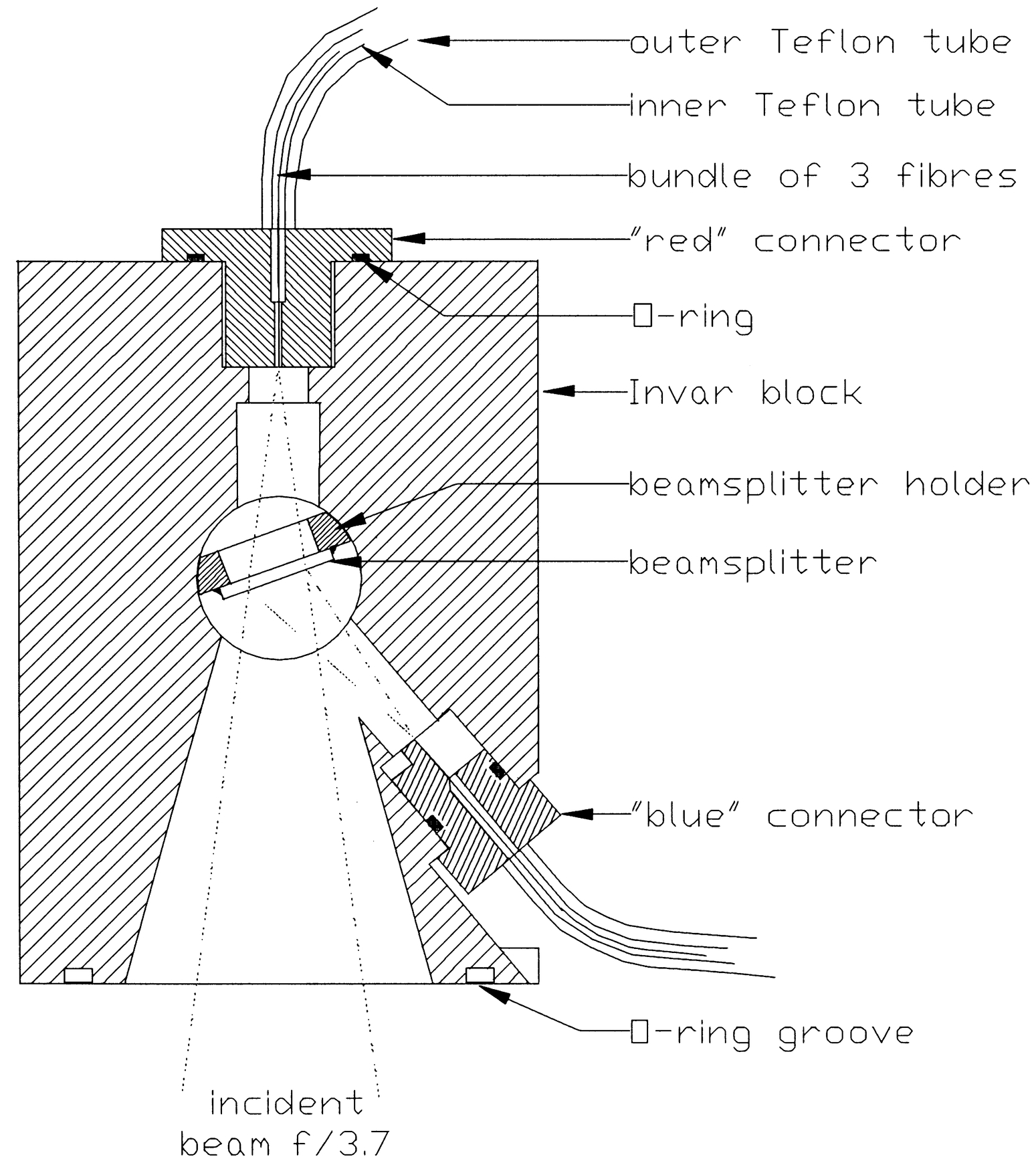
Fig. 4.— Cross section of the optical fiber injection module
After preliminary optical assembly of the telescope tube, the position of the focus relative to the focal plane flange was determined by a Foucault test and was found to be only 500 μm off the design position. Following this measurement, the final longitudinal machining of the injection module was carried out to bring the fibers into perfect focus.
4.2.2. Beamsplitter
A dichroic beamsplitter (BK7 substrate, 10 mm square, 1 mm thick) was made by deposition of a 31 layer coating onto the first surface (R. C. Schaeffer 1996, private communication from A. G. Thompson and Co. Pty. Ltd. [Australia]). We chose a 20° incident angle to minimize the difference in cutoff wavelength between the two polarizations and to reduce astigmatism in the transmitted beam. The disadvantage of this acute angle is an awkward and much reduced space to connect the fibers that are close to the incoming beam. The slope of the cutoff obtained was less steep than expected, with the transmission ranging from 15% at 545 nm to 85% at 656 nm. Its position was also slightly off the specified value with a transmission/reflection ratio of 50% at 592 nm. The glass is glued onto a holder that is inserted into the Invar module from a hole on the side. Ray‐tracing confirmed that astigmatism generated by the glass in the transmitted beam was small (rms and geometric spot sizes were 6.4 and 14 μm, respectively) at 850 nm.
4.2.3. Adjustments
A portable optical bench was built to facilitate the alignment of the fibers in the injection module. One of the blue fibers has to overlap with one of the red fibers when projected back onto the sky, so that a star can be observed simultaneously in both wavelength ranges. We achieve this by back‐illuminating the fibers and observing the output from the injection module with a CCD camera and telephoto lens. The blue fiber connector is fixed with dowels, and the red fiber connector is manually adjusted until alignment is achieved. An overlap of ≥70% can be quickly achieved with this method.
In order not to lose starlight at the entrance of the fiber core, we can afford up to ±0.32 mm of defocus, which is far more than the 0.06 mm thermal deformation from + 20°C to −90°C of the chosen Invar‐Astrositall‐Pyrex combination. Ray‐tracing confirmed that the defocus between the red and blue images was also well within this limit (±0.18 mm around the best focus determined in white light) as both bundles of optical fibers are, by design, equidistant from the beamsplitter.
4.3. Connectors for Optical Fibers
4.3.1. Input
On the telescope side, two brass connectors have been machined to connect the fibers into the injection module. At the extremities of the fibers, the buffer is removed over a few millimeters so that the three claddings can be placed parallel and close together in a rectangular shaped groove. 5‐Minute Araldite epoxy adhesive is used to glue the fibers to the connectors under supervision using a magnifying eyepiece. The precision obtained was about ±20 μm in alignment and with a gap between the fibers of up to 30 μm. Final optical polishing of the connector end was performed to obtain efficient injection of light.
4.3.2. Output
On the spectrograph side, a single brass connector is machined with six V‐shaped grooves separated by 0.8 mm. The same technique as described above is used to glue the fibers. The axes of the six fibers were made parallel with a precision better than 3 ' (the angle between two fiber images on the CCD is 9 ') by careful machining of the grooves.
5. DETECTION SYSTEM
5.1. Spectrograph
We used a commercial imaging spectrograph with a fixed concave holographic grating of 200 g mm−1 from Jobin Yvon (1989) (model CP200). This spectrograph was chosen for its stability (no moving parts) and its excellent stray light rejection ratio (1 part in 104). The entrance beam is f/2.9, which should be close to what we obtain from the FRD in the 45 m of fibers (Avila & D'Odorico 1988; Worswick et al. 1994). The six fibers are mounted in the custom connector described above and are simply positioned at the entrance of the spectrograph, forming a pseudoslit.
The spectrograph focal length is 190 mm and creates a flat image of 25 × 8 mm.
5.2. CCD Camera and Data Acquisition
The CCD camera and controller were built by Oriel Instruments (1995) (model Instaspec IV; open electrode). It has 1024 × 256 pixels (27 × 27μm each, i.e., a total active area of 27.6 × 6.9 mm) with a 16 bit dynamic range. The 100 μm fiber yields a spectral resolution of 2.4 nm FWHM.
We chose to use a central region on the CCD of 5 mm in height. This can accommodate six fibers, separated by 640 μm (24 pixels) along a column to avoid cross talk of spectra on the CCD. The CCD is thermoelectrically cooled by a single air‐cooled Peltier stage able to reach −25°C and consumes about 7 W. The temperature stability (controlled with an accuracy of ±0 5C) is important to ensure that the sensitivity of the CCD is stable with time.
We are using a low‐power PC/104‐based computer (PC/104 is a standard for a compact PC‐compatible module with self‐stacking bus) running under the RTKernel real‐time multitasking operating system. The ERIC software package (Ashley, Brooks, & Lloyd 1996) for remote control over the Internet has been adopted for communication with the AASTO instruments. After being sent via the Internet to UNSW, the data are displayed and analyzed with standard astronomical packages (e.g., IRAF). Every 500 kbyte image is stored on an 800 megabyte hard disk and will be downloaded regularly during the first year for analysis. We can store entire images or just enough of the image to allow extraction of the spectra. In remote regions, where there is no Internet access, we will record the data on the seven 1 gigabyte Iomega "Jaz" drives of the AASTO Data Acquisition Unit.
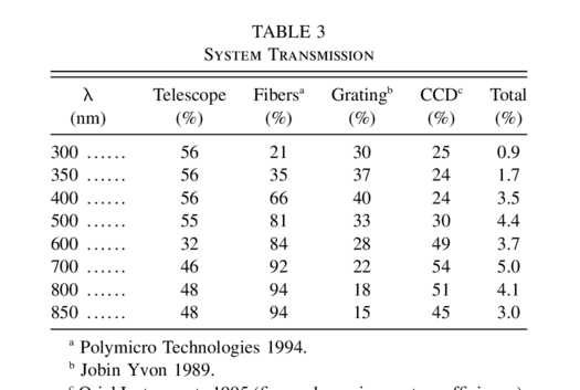
5.3. Overall Transmission
In Table 3, we have grouped under the item "Telescope" all the optical components from the front window to the entrance face of the fibers, including Fresnel loss at each extremity of the fibers.
 |
6. CALIBRATIONS
6.1. Wavelength Calibration
We calibrate the wavelength response of the spectrograph with a mercury lamp and by using the standard Fraunhofer lines in the daytime sky. Features in stellar spectra can also be used.
6.2. Flat‐Fielding
Calibration of the pixel‐to‐pixel response of the CCD is done using a "reference flat" image obtained in the laboratory before shipping the AFOS to Antarctica.
Relative flux calibration is carried out by observing a 10 W quartz‐halogen (QH) bulb mounted on the lower surface of one of the secondary‐mirror support arms. The bulb is an Osram (part number 64415) with a nominal filament temperature of about 3000 K at 12.0 V. The emitted flux as a function of wavelength can be calculated from the appropriate Planck function, modified by the empirically determined emissivity curve for tungsten. We rely on the QH bulb for relative fluxes only; absolute flux will be calibrated at a single wavelength at which the atmosphere is known to be highly transmissive, by observation of standard stars.
The image of the QH bulb on the fibers is completely out of focus, and hence the illumination profile on the fiber is quite different from that of a point source such as a star. However, the broad spectral response of the system (made up of the beamsplitter response, fiber transmission, spectrometer efficiency, and CCD quantum efficiency) is expected to be independent of the fiber illumination pattern. Only the telescope entrance window, which is made of fused silica with well‐determined optical properties, remains outside this calibration process.
The QH bulb is operated at 12 V via a step‐down regulator (Fig. 5) from the nominal 24 V AFOS battery bus. A switching regulator (National Semiconductor Simple Switcher type LM2575‐T12) is used to achieve high‐efficiency (approximately 88%) voltage conversion. In order to maintain a precise voltage across the bulb, independent sense wires are brought back to the regulator from the pins of the bulb. Although the feedback circuitry is very simple, it can stabilize the voltage across the bulb to within ±0.2% over the full anticipated temperature range despite the large voltage drops developed in the long current‐carrying leads to the bulb.
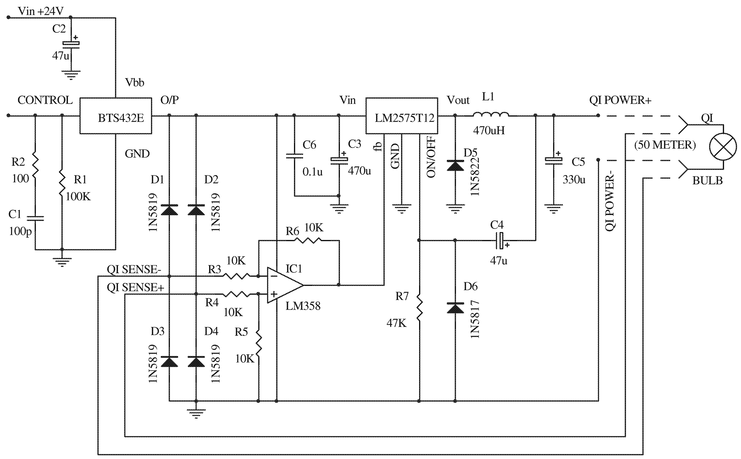
Fig. 5.— Quartz halogen lamp driving circuitry
A final feature of the circuit of Figure 5 is the implementation of a "soft start" by means of C4. When the computer issues a command to turn on the bulb, the BTS432E high‐side switch applies 24 V to the regulator input. As soon as the output voltage of the regulator reaches the threshold of the LM2575 on/off pin (approximately 1.4 V), the regulator stops for a brief period determined by the circuit time constants and the hysteresis in the regulator's internal circuitry. When the regulator restarts, the output rises a small amount and again switches the regulator off via C4. As this cycle repeats, the result is that the output voltage rises very slowly, taking about 30 s to reach 12 V. Once C4 is fully charged, the LM2575 goes into its normal regulation mode, and C4 takes no further part in the operation of the circuit. This soft‐start feature is expected to prolong both the life and the calibration accuracy of the QH bulb, which otherwise would receive a gross thermal shock when switched on cold from as low as −90°C.
7. TESTING AT SIDING SPRING OBSERVATORY
7.1. Alignment
After completion of the manufacturing in 1996 November, the AFOS was taken to Siding Spring Observatory where it was attached to the Automated Patrol Telescope (APT). This allowed us to use the APT's pointing and tracking system for initial tests.
To begin with, we used an eyepiece in lieu of the red fibers to point the AFOS toward Saturn (an easy target with an apparent diameter of 19 ''). The rough accuracy obtained (about 2 ') was enough to inject light successfully into the fiber after a snail scan around the guessed position. We then used a Panasonic video CCD camera (model BP510 with a 75 mm lens), attached to the AFOS tube and bore‐sighted with it, as a reference pointing device.
7.2. Astronomical Spectra
During tests at Siding Spring Observatory, we concentrated on taking spectra (Fig. 6) of bright stars with strong U‐band flux that would be suitable candidates for later comparison in Antarctica. The reduction procedure is standard for spectroscopy with optical fibers: bias level and dark current subtraction, flat‐fielding, fiber aperture extraction, sky subtraction, and finally, flux and wavelength calibration.
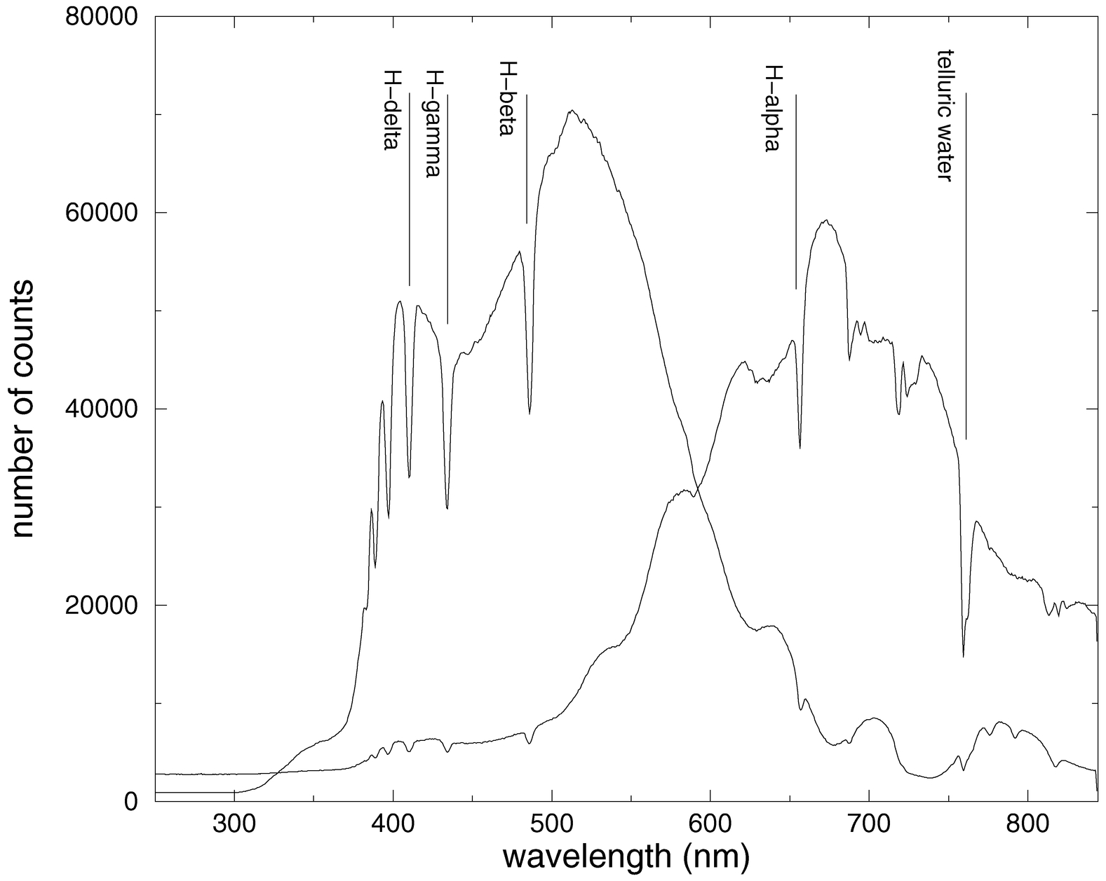
Fig. 6.— Spectrum of Sirius (8 s of integration time) at Siding Spring Observatory. On the vertical scale, one count is equivalent to 12.5 photoelectrons. The left‐hand curve is the blue fiber spectrum, and the right‐hand curve is the red fiber spectrum (whose vertical scale is multiplied by 3 to compensate for poor fiber alignment at that time).
7.2.1. Sensitivity
We have determined the photon flux [N(λ) in photons cm−2 s−1 Å−1] that should reach the CCD using the following assumptions (formula from Zombeck 1990, p. 103):
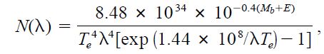
where Te is the effective temperature (in K), E is the atmospheric extinction (we assume 0.4 at a zenith distance of 60° and at 500 nm), and Mb is the bolometric magnitude.
In the following calculation, we use Sirius (an A1 V star) with Mb = -1.69 and Te = 9230 K. With the AFOS collecting surface of 660 cm2, at λ = 500 nm and 60° zenith distance we expect 18.7 × 10⁶ photons s−1 nm−1. Knowing that the instrument transmission is approximately 4% at this wavelength and that the light is spatially spread over 4 pixels (each spectrum represents four lines on the CCD) with a spectral scale of 0.64 nm pixel−1, we finally calculate a flux of 292,000 electrons s−1 pixel−1.
The spectra of Sirius in Figure 6 shows a flux of only about 62,000 electrons s−1 pixel−1 at 500 nm. The mismatch between observation and calculation could be accounted for by factors such as the quality of the injection into the fiber and will be investigated further. However, these unknown losses should not change in time, which should allow us to achieve meaningful photometry.
The minimum airglow intensity at visible wavelengths is typically 1 R (1 R = 106 photons cm−2 s−1 sr−1) or 6.8 × 10⁻¹⁷ W m−2 μm−1 arcsec−2, which is equivalent to a magnitude of 22 arcsec−2. In a 20 '' fiber aperture, we expect to see about 2100 photons s−1 (i.e., 5 electrons s−1 pixel−1).
This is still above the CCD dark current specified of 1 electron s−1 pixel−1 at −25°C, which permits observations limited by the sky background. Furthermore, after only 20 s of integration, the sky photon shot noise becomes dominant over the readout noise (10 electrons per pixel).
7.3. Power Consumption
The complete AFOS instrument draws approximately 15 W at 5 V. This power is principally consumed by the PC/104 computer and the CCD head with its Peltier cooler. In addition, the G‐mount to which the AFOS will be attached is expected to draw up to 25 W. Because the power budget of each instrument in the AASTO is only 7 W, the AFOS will operate with a 15% duty cycle, with energy being stored in small, sealed lead‐acid batteries during the times when the instrument is off. Should the AFOS detect ice on its entrance window, power is sent to the heated window cover for as long as is required to sublime the ice. During this time, the CCD head can be powered down and both the AFOS computer and the G‐mount placed in a "sleep" mode to conserve power.
8. INSTALLATION AT THE SOUTH POLE
The AASTO was commissioned at the South Pole in 1996 December, and the AFOS was installed shortly thereafter in 1997 January (see Fig. 1).
8.1. Tower
The tower was built by the Center for Astrophysical Research in Antarctica (CARA). It is a hexapod construction, 7.5 m high that can be fully assembled and erected without a crane by three people in 2 days. The structure is made from steel beams and rests on compacted snow. Two of the legs are mounted on pivot points on a triangular base, and the third has a ski attached in order to be pulled and raised by a winch. The top platform is about 5 m2 in area and has a built‐in crane to raise and lower the instruments.
8.2. T‐Mount
For the first year of operation, a simplified version of the telescope mount, the T‐Mount, with an elevation drive only, was built by Mount Stromlo and Siding Spring Observatories. Because of the drive limitations, we will concentrate on observing airglow and auroral emissions, do some deicing tests, and experiment with techniques to observe stars (without tracking, they will cross the fibers' FOV in a few seconds, creating a natural shutter).
The future mount, called the G‐Mount (Generic Mount), will also be built at Mount Stromlo and Siding Spring Observatories and is a major technical challenge as it must host two instruments without any maintenance for a period of 12 months, be operational at temperatures down to −90°C, provide ∼20 '' pointing accuracy (down to 2 '' with adaptive tracking), and have a power consumption of less than 25 W.
8.3. Telescope
After installation of the telescope and the mount, we buried a PVC pipe (outside diameter = 100 mm) from the tower to the AASTO shelter. Sections of pipe with angle‐shaped connectors were erected to reach the shelter floor (about 1.2 m above snow level) and along one leg of the tower to reach the upper platform. Finally, the 45 m of optical fibers were pulled slowly through the conduit. Between the telescope focus and the tower platform, the fiber bundles make a large, loose loop around the altitude axis of the mount to permit following the telescope to any position without putting excessive tension in the cables; the same was done for the electrical cables.
The first results of deicing were encouraging and indicated that a window temperature rise of more than 10°C was reached after a few hours of heating at an ambient temperature of −40°C. The few crystals of ice left inside the tube disappeared from the window.
9. FUTURE PLANS
During the austral summer 1997–1998, the telescope will be attached to the new motorized alt‐az G‐Mount. It will have the capability to point at any star. There are also plans to build a new tower (14 m high), possibly fabricated from carbon fiber.
After the second year of testing at the South Pole, the AASTO will be moved to higher sites beginning with Dome C (3200 m, 75° south, 124° east). Ultimately we hope to be able to investigate Dome A (4200 m, 81° south, 78° east). We will then have valuable comparisons between these most promising locations. The site testing campaign will allow a definitive assessment of where in Antarctica a major astronomical observatory should be built and what performance could be expected.
We owe a great debt to many people for the completion of this instrument. We particularly thank Howard Roscoe for his advice leading us to the choice of some major components and Keith Taylor for facilitating the collaboration with Greg Smith and Allan Lankshear, engineers at the AAO. We also received important support from many other people at the AAO and MSSSO during fabrication and testing in Australia. Thanks to Nick Roberts for his advice on the chemistry of CaH2, Sun Yin Sheng for his work on the mechanical analysis, and Michael Burton for his encouragement and advice on the scientific issues. We thank the different workshops on the campus of UNSW for completing the work on time. We are very grateful to Bob Pernic and his team from CARA for building the wonderful hexapod tower and their assistance during the critical set up at the South Pole. The AFOS was funded by the Australian Antarctic Foundation and the Australian Research Council. Finally, we thank the US National Science Foundation for supporting the recent visit of our team to the South Pole and Paul Sullivan for his invaluable assistance throughout the South Pole winter. Deployment and operation of the AASTO is supported by the US National Science Foundation under a cooperative agreement with CARA, grant NSF OPP 89‐20223. CARA is a National Science Foundation Science and Technology Center.
Footnotes
- 1
All the thermal expansion coefficients quoted in the text are valid at room temperature and have low variation (≤10%) over the range +20°C to −90°C.