


The bifurcation and Lyapunov exponent for a single-machine-infinite bus system with excitation model are carried out by varying the mechanical power, generator damping factor and the exciter gain, from which periodic motions, chaos and the divergence of system are observed respectively. From given parameters and different initial conditions, the coexisting motions are developed in power system. The dynamic behaviors in power system may switch freely between the coexisting motions, which will bring huge security menace to protection operation. Especially, the angle divergences due to the break of stable chaotic oscillation are found which causes the instability of power system. Finally, a new adaptive backstepping sliding mode controller is designed which aims to eliminate the angle divergences and make the power system run in stable orbits. Numerical simulations are illustrated to verify the effectivity of the proposed method.
I. INTRODUCTION
Chaotic oscillations in power systems may cause a lot of complex nonlinear dynamic behaviors, which may present some potential threats to the safe operation of the power grid. In 1988, Salam1 calculated the homoclinic orbit in a two-machine system which illustrates the existence of chaotic motions in power systems. Since then, many researchers began to focus on the study of chaos in power systems. In 1993, the existence of chaos for a simple power system was first confirmed through the calculation of Lyapunov exponents and broad-band spectrum.2 The nonlinear phenomena3 were observed in a single-machine-infinite-bus power system with the excitation hard-limits, and the global bifurcations including period-doubling cascades which leaded to chaotic behavior were observed. Yu et. Al.4 focused on three routes to chaos including the period-doubling bifurcation, torus bifurcation directly initiated by a disturbance of energy, and also revealed that chaos can lead power system to voltage collapse and angle divergence. Subramanian5 developed the bifurcation diagrams of steady state solutions in a power system from which the existence of various bifurcation points such as Hopf bifurcation, fold bifurcation, saddle-node bifurcation and period-doubling bifurcation were obtained, and voltage collapse and chaotic motions due to period doublings were also unearthed. Qin6 studied the effect of the dynamical behaviors in a simple power system with random parameter. Furthermore, with the expansion of the social power demand, the scale of power systems become gradually increasing. The important features of modern power systems are high-voltage and long-distance transmission, for which the systems often operate near their stability limits. The research on chaotic motion and stability of the power systems become extremely urgent.
According to the above researches, chaotic motions are easily observed in the power systems with the change of system parameters and random disturbances. For the general systems, the chaotic trajectory of system will have a great difference with the different initial value but their final steady state is still same. However, for the complicated power systems, the trajectories and final stable state will be influenced with the tiny changes of the initial value, which implies the power systems have the ability to exhibit a number of coexisting motions for a given system parameters. This phenomenon, called multistability, has been observed in many fields of science.7–9 Venkatasubramanian and Ji10 reported four attractors coexisted phenomena in a power system, but no detail report on bifurcation and Lyapunov with changing parameters of system was given. Ma and Min11 also investigated the coexistence of periodic orbits and chaos in a delayed power system. The existing phenomenon increases the complexity of the system and brings huge threaten to the stability of the power grid. With the break of chaotic oscillations or the coexistence of different motions, the angle divergence and voltage collapse in power system will be taken place.
Therefore, it is necessary to design controllers to prevent the instability of power system. So far a lot of control methods have been studied to suppress chaotic oscillation in power system. Wei12 designed an adaptive controller based on the LaSalle invariance principle to suppress different undesirable bifurcations which threatened the secure and stable work of power system. Li13 proposed a robust adaptive fuzzy controller for a single machine bus system through static var compensator. Furtat14 investigated the robust control of multi-machine power systems with parameters uncertainties. Min15 designed a controller through the relay characteristic function to suppress chaotic motions in interconnected power system. Ni16 proposed the variable speed synergetic controller to eliminate chaotic oscillation in power system.
In this paper, the nonlinear dynamics of a single-machine-infinite bus system is studied through the bifurcation diagrams and Lyapunov exponent. The coexistence of different motions as well as the instability in power system is observed due to angle divergence. Moreover, to eliminate chaotic motions in nonlinear power system, an adaptive backstepping sliding mode controller is proposed, which can guarantee that the angle and frequency of power system keeps operating on the stable orbit. Compared to other controllers, the adaptive backstepping sliding mode controller has the advantage of adaptive backstepping control and sliding mode control which possesses more robustness to uncertainties for the tracking targets.
II. THE POWER SYSTEM MODEL
A single-machine-infinite bus system with the excitation limitation3 is presented in Fig. 1, which consists of generators, transformer, load, circuit breaker, systematic tie line and the simplified excitation model.
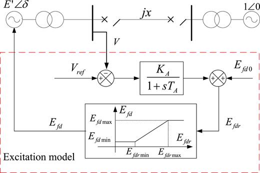
The single-machine-infinite bus system can be described as
where Efdr is the input signal of wind-up limiter and the output of the wind-up limiter Efd is shown as
and the bus voltage at the generator bus terminal is defined as
where δ is the generator angle, ω is the machine frequency, E′ is the generator voltage behind the transient reactance, H is the moment of inertia in second, D is the generator damping factor, Pm is the mechanical power, V0 is the infinite bus voltage, x denotes the transmission line reactance, xd denotes the synchronization reactance, represents the transient reactance, is the open-loop time constant of the armature winding, Vref is the reference bus voltage, TA is the time-constant, KA is exciter gain and Efd0 is the reference voltage. The power system10 can exhibit periodic orbits, stable chaos and the instable divergence motions with varying the system parameters Pm, D and KA.
III. DYNAMIC ANALYSIS OF POWER SYSTEM WITH EXCITATION LIMITATION
In this section, through the typical bifurcation diagrams and Lyapunov exponents, the nonlinear dynamics in power system is analyzed to illustrate the effects of mechanical power Pm, generator damping factor D and exciter gain KA. The coexistence of attractors in nonlinear systems often appear with the same parameter values with different initial conditions, which presents interesting characterics of multistable system. The route to chaos in power system in Eq. (1) is due to the period-doubling bifurcation (i.e., PDB), and the coexisting motions of different periodic-orbits are also observed. The instability of power system is caused by the angle divergence when stable chaotic oscillation is destroyed. The initial conditions, i.e, IC1 = (0.98571, -0.0004, 1.4046, 2.3282), and IC2 = (1.4378, 0.0032, 1.3389, 10.9338) in the simulations are given, respectively. The system parameters is fixed by
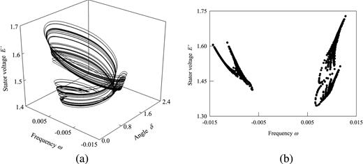
The mechanical power Pm has a great influence on stable operation in power system with excitation limitation, which determines the speed of the generator. To better understand the dynamics of power system in Eq. (1), the bifurcation diagrams and Lyapunov exponents with the parameter Pm ∈ [1.036, 1.304] are shown in Fig. 2(a) and 2(b) respectively with D = 1.4 and KA = 150. The chaotic and periodic motions of power system can be easily observed. From Fig. 2(b), the largest exponent with increasing parameter Pm is negative for Pm ∈ [1.036, 1.2982] in which different periodic motions are presented in Fig. 2(a), while the largest exponent for Pm ∈ [1.2982, 1.301] is larger than zero, which means that chaotic motions exist. The coexisting domain of period-1 and perod-2 lies in Pm ∈ [1.0401, 1.1025] with the hatched areas for the different initial conditions, while the same motions with IC1 and IC2 are observed for the other ranges. Black dots mean the trajectories with the initial condition IC1, and red dots denote the trajectories with the initial condition IC2. The phase portraits of the coexistence at Pm = 1.05 are shown in Fig. 3(a) and 3(b). From Fig. 2(a), a switch ‘jump’ motion from period-1 to period-2 can be observed in Pm ∈ [1.1025, 1.1029] because of the non-smooth wind-up limiter. From a small periodic window in Fig. 2(a), a PDB period-doubling bifurcation is observed at Pm = 1.29403, and then periodic-4 motions appear until another PDB occurs at Pm = 1.29773. Next, the single-machine-infinite bus system begins to enter into chaotic motions at Pm = 1.2982 after a series of PDB, and four Lyapunov exponents with Pm = 1.2982 are (0.1358, 0.0, -0.1028, -1.346) in Fig, 2(b). The chaotic trajectories of power system in Eq. (1) are depicted in Fig. 4(a) with parameters Pm = 1.3, D = 1.4 and KA = 150, and the corresponding Poincaré maps are presented in Fig. 4(b) which consist of many irregular points. Finally, with the mechanical power increasing from Pm = 1.301, the strange attractor grows larger and then disappears, which indicates the extinction of chaotic motions at a boundary crisis. In Fig. 5(a), the transient chaotic behavior for Pm = 1.305 is displayed by initially staying at t = 30.1s, and then the stable chaotic motion is broken. The machine angle δ increases monotonously along the trajectories from Fig. 5(b) so that the generator loses synchronism possibly leading to a power system break-up. The stator voltage is better behaved along the divergence while the angle quickly diverges away with any initial conditions. Thus, the collapse of power system is only caused by the machine angle instability.
![FIG. 2. Bifurcation diagram(a) and Lyapunov exponent(b) in power system for Pm ∈ [1.036, 1.304], D = 1.4 and KA = 150.](https://aipp.silverchair-cdn.com/aipp/content_public/journal/adv/6/8/10.1063_1.4961696/4/m_085214_1_f2.jpeg?Expires=1716296907&Signature=nIyqrBWyFuDD2S8Fj2c3KXmbZ57IdDZDHrML4xYZUdrbNY5grBkwMlgc5EGqUw84iVBNIV2Aa9dX7j05w3Fi-1vwhGd1Tl~MLV4tft8fNctiA4kSCXzcZCjfwk2ib3fE17BBZ0A9LtN3gHoEu6NGAAKgim4cG26IC~FLArPzs968ofmxcaDdOooJkhSWZE~5kjABq53hs1lleLwQ9lBVwLjArQk3KbF1g8bYnTBeBBT~D8tb6uOkXbs6Rrh--AVhSGryhKowciMohRpAyaq13~HwoxwFSQgSjvqGh4LNDjjBermt1I-7NK4hPRCtkeY4AHm~FaKjfZ8dkjzA88bwXw__&Key-Pair-Id=APKAIE5G5CRDK6RD3PGA)
Bifurcation diagram(a) and Lyapunov exponent(b) in power system for Pm ∈ [1.036, 1.304], D = 1.4 and KA = 150.
Bifurcation diagram(a) and Lyapunov exponent(b) in power system for Pm ∈ [1.036, 1.304], D = 1.4 and KA = 150.
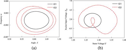
The coexistence of Period-1 and Period-2 in power system for Pm = 1.05, D = 1.4 and KA = 150 with different initial conditions: (a) (δ, ω), (b) (E′, Efdr).
The coexistence of Period-1 and Period-2 in power system for Pm = 1.05, D = 1.4 and KA = 150 with different initial conditions: (a) (δ, ω), (b) (E′, Efdr).

The swift divergence of machine angle for the single machine infinite bus system for Pm = 1.305, D = 1.4 and KA = 150: (a) phase trajectories, (b) time-historical machine angle. (The red arrow means the direction of motion.).
The swift divergence of machine angle for the single machine infinite bus system for Pm = 1.305, D = 1.4 and KA = 150: (a) phase trajectories, (b) time-historical machine angle. (The red arrow means the direction of motion.).
Next, it is necessary to analysis the dynamical behaviors with a damping parameter for which model the overall damping effects in the power system. The bifurcation diagrams and Lyapunov exponents are presented for D ∈ [1.36, 5.08], P = 1.3 and KA = 150 in Fig. 6(a) and 6(b). The coexisting region in D ∈ [2.79, 3.84] is hatched with two period-2 motions for the initial conditions IC1 and IC2, while the other regions show the same behaviors. The coexistence of period-2 and period-2 with different initial conditions is plotted at D = 2.9 in Fig. 7. Time-historical machine angle δ and exciter input voltage Efdr display two period-2 motions with varying time which agree with the bifurcation in Fig. 6(a). With the damping factor decreasing from 5.08, the different periodic motions first occur in the range D ∈ [1.433, 5.08] from Fig. 6(a), and the largest Lyapunov exponent approaches near zero or becomes negative in Fig. 6(b). Then the power system at D = 1.433 enters into the chaos through a series of PDB, and the corresponding four Lyapunov exponents with D = 1.433 are (0.1192, 0.0, -0.098, -1.334) in Fig. 3(b). Finally, the machine angle will tend to infinite with decreasing D = 1.389, which illustrates that the instability of power system with the damping factor dropping off occurs.
![FIG. 6. Bifurcation diagram(a) and Lyapunov exponent(b) of the single machine infinite bus system forD ∈ [1.36, 5.08] with Pm = 1.3, KA = 150.](https://aipp.silverchair-cdn.com/aipp/content_public/journal/adv/6/8/10.1063_1.4961696/4/m_085214_1_f6.jpeg?Expires=1716296907&Signature=HSqBgBAL47klaMbossdiGBwelcRPT9p9YZI8xSLEafZ8-wP0BxHtpQ4~YV6SV6VNVxPaY3zu039TnNWbFl9miPzoVnHgff4OO14IXotb23ZbqiJos5ocrXjO45WIBRON7dZ7b8wCHy7RMSwuUkV5zPLainvJoR-Evrmv7HSnZG0y8AVomlRMXwLLfceuukY-qPBwrmeWcvpSQ5JuUxTk51QyIoHCcUmR9tFT0xNFPUPEN46oD6bY-M8PsA6Xya~CaGR~FgrgSG4~7qETwxJGd0HWeQtY2prS51vS0vBWHE0Zfz09FgnCUmwZ~sFvDsrA4kJruWCTA5zO7-GwDSI-Hw__&Key-Pair-Id=APKAIE5G5CRDK6RD3PGA)
Bifurcation diagram(a) and Lyapunov exponent(b) of the single machine infinite bus system forD ∈ [1.36, 5.08] with Pm = 1.3, KA = 150.
Bifurcation diagram(a) and Lyapunov exponent(b) of the single machine infinite bus system forD ∈ [1.36, 5.08] with Pm = 1.3, KA = 150.
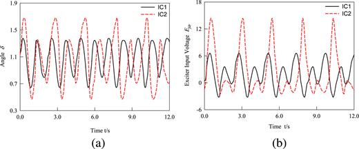
Two different Period-2 orbits with different initial conditions for Pm = 1.3 and D = 2.9: (a) time-historical machine angle δ, (b) time-historical Exciter Input Voltage Efdr.
Two different Period-2 orbits with different initial conditions for Pm = 1.3 and D = 2.9: (a) time-historical machine angle δ, (b) time-historical Exciter Input Voltage Efdr.
Furthermore, the bifurcation diagrams and Lyapunov exponents for with Pm = 1.3 and D = 1.4 are represented in Fig. 8. The coexisting regions of two different period-1 are shown in KA ∈ [84.21, 87.86], and the coexistence of period-1 and period-2 orbits is also given in KA ∈ [87.86, 92.01] with IC1 and IC2. The same behaviors of power system with two different initial conditions occur for the remaining range of the exciter control gain KA > 92.01. In Fig. 8, two ‘jump’ motions at KA = 87.86 and KA = 92.01 are observed from period-1 to period-2, which often takes place in discontinuous systems. From Fig. 7, the power system runs at stable equilibrium points for the exciter gain KA < 84.21 and all Lyapunov exponents are less than zero. The periodic windows are observed in KA ∈ [84.21, 141], which is in agreement with the largest Lyapunov exponent. With parameters KA increasing from 84.21, period-2 orbits suddenly turn to period-4 orbits because PDB occurs at KA = 123.45, and then period-8 motions appear until another PDB is found at KA = 138.43. Next, the stable periodic behaviors disappear and chaotic motions begin to appear from KA = 141 due to the crisis of the boundaries, and four Lyapunov exponents with KA = 141 are (0.0134, 0.0, -0.097, -1.215) in Fig. 8(b). The gain of the excitation limitation in power system determines the stability of the generator, which often has high control values for KA. When the gain KA is increased from 141, the strange chaotic attractors become larger and may eventually hit the unstable limit set, resulting in the broken of chaos at KA = 151.3. Time-plots histories of the trajectories for the power system are presented in Fig. 9 with the parameters Pm = 1.3, D = 1.4 and KA = 170. In this case, only the machine angle monotonously increases and is quick divergent while the machine frequency ω, the generator voltage E′ and the input signal of wind-up limiter Efdr quickly conerge to the equilibrium points which form the local stable space. Obviously, the unstable power system is caused by the divergence of machine angle without voltage collapse.
From the above discussions, the complex dynamics of the power system are investigated by changing the system parameters, and the coexisting regions, periodic motions and chaos are observed, respectively. The instability of system is caused by the divergence of machine angle because of the broken chaos. Therfore, it is necessary to design an effective controller to suppress the instability, chaos and the coexisting phenomenon in power system.
![FIG. 8. Bifurcation diagram(a) and Lyapunov exponent(b) of the single machine infinite bus system KA ∈ [80, 152] with Pm = 1.3 and D = 1.4.](https://aipp.silverchair-cdn.com/aipp/content_public/journal/adv/6/8/10.1063_1.4961696/4/m_085214_1_f8.jpeg?Expires=1716296908&Signature=EAeQPlSGLSY6enCfWqVto-x2LAOvIqrDzcTsYw16l8lmfyXS7Fvsl~viXy3cVo~XK0mHEF8sHqnckxDS-rDecq19LJxHqAV7LnXx7jfu9I9Fvkn~D8ND9zXCARSIqGiIw-cZ5laViE3iYQrBdJuE-7UMBpmsnoQ3PT7YVEmNlMogEqTOb2vf41y1bbpYKu-0q4zTE7Sg4XWrRKKaESHAOk9h3ptssZoudEJqI2HEUJikc0eseqVqBEFAINQ1TEkQJA0gSGhiva48jRWRdTEtNyLYvXj8AVM5i8oE43Lura~8BODoEIKTgyi3DMBbhyGYyusLhJ2kJYaD0oa-EcLvUQ__&Key-Pair-Id=APKAIE5G5CRDK6RD3PGA)
Bifurcation diagram(a) and Lyapunov exponent(b) of the single machine infinite bus system KA ∈ [80, 152] with Pm = 1.3 and D = 1.4.
Bifurcation diagram(a) and Lyapunov exponent(b) of the single machine infinite bus system KA ∈ [80, 152] with Pm = 1.3 and D = 1.4.

Numerical simulation results for the instability of the single-machine-infinite bus system for Pm = 1.3, D = 1.4 and KA = 170:(a) time-historical machine angle δ, (b) time-historical frequency ω, (c) time-historical Stator Voltage E′, (d) time-historical Exciter Input Voltage Efdr.
Numerical simulation results for the instability of the single-machine-infinite bus system for Pm = 1.3, D = 1.4 and KA = 170:(a) time-historical machine angle δ, (b) time-historical frequency ω, (c) time-historical Stator Voltage E′, (d) time-historical Exciter Input Voltage Efdr.
IV. ADAPTIVE BACKSTEPPING SLIDING MODE CONTROL
To eliminate chaotic oscillation in power system, an adaptive backstepping sliding mode controller with a simple adaptive law is proposed to keep the power system operating on a stable motion. The operational control variable in a power system can be accessible, and the control objective must be implementable easily in engineering. The machine angle δ of the generator often can be controlled at the desired value when the system is unstable, which is often the control object. The input signal of wind-up limiter Efdr and the output of the wind-up limiter Efd are used to change the voltage in power system, which needn’t be controlled. Thus the control objective is to propose an adaptive backstepping sliding mode control system for the output angle of power system to track the given target asymptotically. Now the designed controller u is added to the second equation of system Eq. (1), and the controlled system can be rewritten by
The adaptive backstepping sliding mode controller design procedure is shown as follows:
Step 1: Define the target as r and the output as δ, and the tracking error as
and its derivative is given by
The first Lyapunov function is described as
Let be the virtual control. The expression becomes . The time derivative of V1 along with Eq. (7) is
The switching function of sliding mode control is defined as
and the parameters k1, c1 are positive. Obviously, if the switching function σ = 0, then e1 = e2 = 0 and .
Step 2: To design the controller u, the mechanical power Pm and the effect of excitation limitation in power system denote the total uncertainties. Thus the second equation of system Eq. (5) can be shown as
where F denotes the lumped uncertainty, which is assumed to be bounded, i.e., . The upper bound M is a positive constant which is difficult to obtain, therefore, the estimate value of lumped uncertainty is given by . Then the Lyapunov function is chosen
where γ is a positive constant and the error of estimation is .
According to Eq. (13), an adaptive backstepping sliding mode controller is designed as
where both h and n are positive constants. The adaptive law for is designed as
where eT = [e1 e2] and Q is a symmetric matrix with the form
To guarantee that Q is positive definite, the following conditions should be held by
where h, c1, k1 are positive constants. A sufficient condition to guarantee that Q is positive definite is as follows
According to Barbalat’s lemma, the expression will converge to zero when time t approaches to infinite. Therefore, the error e1 and e2 will also tend to zero as t → ∞. Finally, the stability of the adaptive backstepping sliding mode control system can be proved.
To avoid the chattering phenomena, the following relay characteristic function can be used to replace the sign function in Eq. (14) in numerical simulations
where
and r0,s0 are small positive constants.
To illustrate the effects of the designed adaptive backstepping sliding controller, the following two cases are considered as the target r = 1.0 and r = 0.1sin(2t) + 1.0, respectively. In the simulation, the chaotic oscillation in power system is shown with parameters Pm = 1.3, D = 1.4 and KA = 150. At this time, the controller u is put into effect at t =20s. Simulation results are depicted in Fig. 10, and the design parameters are given by c1= 10, k1 = 15 h = 25 and n = 1.5. From Fig. 10(a) and 10(b), it is observed that the chaotic motions in power system can be quickly tracked to the object for t ≥ 20s, respectively, which indicates that the proposed control method can restrain chaos and render the controlled power system asymptotically stable.
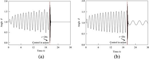
Time responses of the controlled single machine infinite bus system with the control gains c1 = 10, k1 = 15 h = 25 and n = 1.5: (a) the target r = 1 and (b) the target r = 0.1sin(2t) + 1.0 for the chaotic motion with parameters Pm = 1.05, D = 1.4 and KA = 150.
Time responses of the controlled single machine infinite bus system with the control gains c1 = 10, k1 = 15 h = 25 and n = 1.5: (a) the target r = 1 and (b) the target r = 0.1sin(2t) + 1.0 for the chaotic motion with parameters Pm = 1.05, D = 1.4 and KA = 150.
V. CONCLUSIONS
In this paper, the bifurcation diagrams and Lyapunov exponent in the power system are investigated by varying the different system parameters, in which the coexisting periodic motions and chaotic oscillation are observed. Simulation results are plotted with the phase portraits, Poincaré maps and the time-historic responses. The coexistence of period-1 with period-1 orbits, and period-2 with period-1orbits are observed with different initial conditions. The instability of power system is also observed when the machine angle becomes larger and larger for the broken of chaos. Therefore, in order to hold back the collapse of power system and guarantee the power system operates at a desire value, the adaptive backstepping slide mode controller is designed to eliminate chaotic oscillations. Finally, the effectiveness of the designed control scheme has been confirmed by the simulations.
ACKNOWLEDGMENTS
The work is supported by the National Natural Science Foundation of China (No. 51475246) and the Natural Science Foundation of Jiangsu Province under Grant No Bk20131402.

